Current and future supernova constraints on decaying $\Lambda$ cosmologies

Abstract

We investigate observational constraints from present and future supernova data on a large class of decaying vacuum cosmologies. In such scenarios the present value of the vacuum energy density is quantified by a positive $\beta$ parameter smaller than unity. By assuming a Gaussian prior on the matter density parameter ($\Omega_{\rm{m}}=0.35\pm 0.07$) we find $\Omega_{\rm{m}}=0.34^{+0.14}_{-0.12}$ and $\beta=0.62^{+0.12}_{-0.24}$ ($95\%$ c.l.) as the best fit values for the present data. We show that, while the current data cannot provide restrictive constraints on the $\Omega_{\rm{m}}-\beta$ plane, the future SNe data will limit considerably the allowed space of parameter. A brief discussion about the equivalence between dynamical-$\Lambda$ scenarios and scalar field cosmologies is also included.

I Introduction

A large number of astronomical observations have led to a resurgence of interest in a Universe dominated by a relic cosmological constant ($\Lambda$). The basic set of experiments includes the luminosity distance measured from type Ia supernova (SNe Ia) perlmutter ; riess , measurements of cosmic microwave background (CMB) anisotropies bern , clustering estimates calb , age estimates of globular clusters carreta and high-redshift age estimates dunlop . It is believed that the presence of an unclustered component like the vacuum energy not only explains the observed accelerated expansion but also reconciles the inflationary flatness prediction ($\Omega_{\rm{Total}}=1$) with the $\Omega_{\rm{m}}$ measurements that point sistematically to a value between $\Omega_{\rm{m}}=0.2-0.4$.

On the other hand, it is also well known that the same welcome properties that make models with a relic cosmological constant ($\Lambda$CDM) our best description of the observed universe also result in a serious fine tuning problem wein . The basic reason is the widespread belief that the early universe evolved through a cascade of phase transitions, thereby yielding a vacuum energy density which is presently 120 orders of magnitude smaller than its value at the Planck time. Such a discrepancy between theoretical expectations and empirical observations constitutes what is usually called “the cosmological constant problem”, a fundamental question at the interface uniting astrophysics, cosmology and particle physics.

As a phenomenological attempt of alleviating such a problem, the so-called dynamical-$\Lambda$ or decaying $\Lambda$ cosmologies were originally proposed in ozer . Afterwards, a number of different scenarios with suggestive decaying laws for the variation of the cosmological term were investigated ozer1 (see also over for a review). In Refs. jackson ; lima1 the authors proposed a class of deflationary cosmologies driven by a decaying vacuum energy density whose present value, $\Lambda_{o}$, is a remnant of a primordial deflationary stage. Such models are analytic examples of warm inflation scenarios proposed more recently by Berera WI in which particle production occurs during the inflationary period and, as consequence, the supercooling process, as well as the subsequent reheating are no longer necessary. The basics of the cosmological history of such models can be summarized as follows jailson : first, an unstable de Sitter configuration is supported by the largest value of the vacuum energy density. This nonsingular state evolves to a quasi-Friedmann-Roberton-Walker (FRW) vacuum-radiation phase and, subsequently, the Universe approaches continuously to the present vacuum-dust stage. The first stage harmonizes the scenario with the cosmological constant problem, while the transition to the second stage solves the horizon and other well-know problems in a similar manner as in inflation. Finally, the Universe enters in the present accelerated vacuum-dust phase as apparently suggested by the SNe Ia observations. Other specific examples of exact deflationary models and the underlying thermodynamics have been studied recently by Gunzig et al. GMN . Some scalar field motivated descriptions for this class of models were investigated in Refs. maar ; zimd ; jackson1 .

From the observational viewpoint some analyses have indicated a good agreement between these models and different classes of comological tests joao . For example, Bloomfield Torres and Waga tw analysed gravitational lensing constraints on a scenario in which the cosmological term decreases with time as $\Lambda\propto R(t)^{m}$, where $R(t)$ is the scale factor and $m$ is a free parameter in the interval $0\leq m\leq 3$. They found that for low values of $\Omega_{\rm{m}}$ there is a wide range of values of $m$ for which the lensing rate is considerably smaller than in the conventional $\Lambda$CDM models. In particular, for values of $m\geq 1$, these models reproduce very well the observed lens statistics in the Hubble Space Telescope Snapshot Survey. More recently, Vishwakarma vish investigated some $\Lambda(t)$ models in the light of SNe Ia data and measurements of the angular size of compact radio source ($\theta(z)$). The same $\theta(z)$ data together with age constraints from globular clusters and high-$z$ galaxies were also analysed by Cunha et al. jailson in the context of deflationary scenarios. In all of these cases, a good agreement between theory and observations was found.

The aim of the present paper is twofold: first, to investigate the observational contraints from the current SNe Ia data on the class of deflationary cosmologies proposed in jackson ; lima1 and compare them with other recent results; second, to simulate future SNe Ia data to infer how restrictive will be the limits on the decaying rate $\beta$ from these high quality data. By future SNe Ia data we assume a large number of high-$z$ supernova that will become available from the projected Supernova/Acceleration Probe (SNAP) satelite mission snap . Such data have been explored in the recent literature by several authors aiming mainly at determining a possible time or redshift dependence of the dark energy al . A scalar field description for our dynamical-$\Lambda$ scenarios is also discussed.

This paper is organized as follows. In the next section we present the basic field equations relevant for our analysis. In Sec. III we discuss a procedure to find scalar field counterparts for the decaying-$\Lambda$ cosmologies studied here which share the same dynamics and temperature evolution law. The corresponding constraints for deflationary cosmologies from the current SNe Ia data are investigated in Sec. IV. In Sec. V we discuss the improvements in the parameter estimation by simulating the future SNAP data. We end this paper by summarizing the main results in the conclusion section.

II The model: basic equations

For homogeneous and isotropic cosmologies driven by nonrelativistic matter plus a cosmological $\Lambda(t)$-term the Einstein field equations are given by

$$8\pi G\rho+\Lambda(t)=3\frac{\dot{R}^{2}}{R^{2}}+3\frac{k}{R^{2}}\quad,$$ (1)

$$\Lambda(t)=2\frac{\ddot{R}}{R}+\frac{\dot{R}^{2}}{R^{2}}+\frac{k}{R^{2}}\quad,$$ (2)

where an overdot means time derivative, $R(t)$ and $k=0,\pm 1$ are, respectively, the scale factor and the curvature parameter and $\rho$ stands for the dust energy density.

In this kind of deflationary cosmologies, the effective $\Lambda(t)$ term is a dynamic degree of freedom that relaxes to its present value, $\Lambda_{o}$, according to the following ansatz lima1

$$\rho_{v}=\frac{\Lambda(t)}{8\pi G}=\beta\rho_{T}\left(1+\frac{1-\beta}{\beta}{H\over H_{I}}\right)\quad,$$ (3)

where $\rho_{v}$ is the vacuum density, $\rho_{T}=\rho_{v}+\rho$ is the total energy density, $H={\dot{R}}/R$ is the Hubble parameter, $H_{I}^{-1}$ is the arbitrary time scale characterizing the deflationary period, and $\beta\in[0,1]$ is a dimensionless parameter of order unity. As shown in jackson ; jailson , regardless the choice for the begining of the deflationary process, the scale $H_{I}$ is unimportant during the vacuum-dust dominated phase ($H<<H_{I}$) so that, for all practical purposes at the late stages of the cosmic evolution, the vacuum energy density (Eq. 3) can be approximated by $\rho_{v}=\beta\rho_{T}$. It is worth mentioning that only for flat scenarios $\beta$ can be considered identical to the vacuum energy density $\Omega_{\Lambda}$. From Eqs. (1) and (3) it is possible to show that the general relation between these two parameters is given by $\Omega_{\Lambda}=\beta[1+k/(RH)^{2}]$.

By combining the above equations, we see that the deceleration parameter, usually defined as $q_{o}=-R\ddot{R}/\dot{R}^{2}|_{t_{o}}$, now takes the following form

$$q_{o}=\frac{\Omega_{\rm{m}}}{2}\frac{(1-3\beta)}{(1-\beta)}$$ (4)

or still, in terms of the curvature parameter $k$,

$$q_{o}={1-3\beta\over 2}\left[1+{k\over(R_{o}H_{o})^{2}}\right],$$ (5)

which clearly reduces to the standard relation $q_{o}=\frac{\Omega_{\rm{m}}}{2}$ in the limit $\beta\rightarrow 0$. As can be seen from the above equation, for any value of $\Omega_{\rm{m}}\neq 0$, the deceleration parameter with a decaying vacuum energy is always smaller than its corresponding in the standard context and the critical case, $\beta=1/3$ ($q=0$), describes exactly the class of “coasting cosmologies” studied in kolb .

III Scalar Field Version

A procedure to find scalar field counterparts for flat decaying-$\Lambda$ cosmologies sharing the same dynamics and temperature evolution law has been recently proposed jackson1 . In this Section, we extend such a procedure to write the necessary equations of a “coupled quintessence” cquint version for the late time behavior of the arbitrary $k$ cosmology considered here.

Firstly, we extend the analysis of Ref. jackson1 and use Eqs. (1)-(3) in the limit $H/H_{I}\to 0$ (our present time universe) to define the parameter

$$\gamma_{*}\equiv-{2\dot{H}\over 3H^{2}}=(1-\beta)\left(1+{k\over(RH)^{2}}\right).$$ (6)

The above equation is just another way of writting the field equations, so that any cosmology dynamically equivalent to the asymptotic decaying-$\Lambda$ model considered here must have the same $\gamma_{*}$. Perhaps this fact can be made more explicit if one considers that such a parameter is directly related to the deceleration parameter:

$$\gamma_{*}={2\over 3}(q+1).$$ (7)

From Eqs. (1)-(3) it can be found that

$$H^{2}+{k\over R^{2}}=AR^{-3(1-\beta)},$$ (8)

where the integration constant $A=(8\pi G/3)\rho_{T0}R_{0}^{3(1-\beta)}$. Another useful parameter necessary to simplify the notation of the scalar field equations is

$$x\equiv{\dot{\phi}^{2}\over\dot{\phi}^{2}+\rho-2k/3(RH)^{2}},$$ (9)

which reduces to the $x$ parameter used in jackson1 for $k=0$. In the above equation, $\phi$ is a minimally coupled scalar field and, as indicated earlier, an overdot denotes time derivative. Now, if we define the scalar field energy density and pressure:

$$\rho_{\phi}={\dot{\phi}\over 2}+V(\phi)\quad\mbox{and}\quad p_{\phi}={\dot{\phi}\over 2}-V(\phi),$$

respectively, and replace in Eqs. (1) and (2) the vacuum energy density and “pressure”

$$\rho_{v}=\Lambda/8\pi G\to\rho_{\phi}\quad\mbox{and}\quad p_{v}=-\Lambda/8\pi G\to p_{\phi},$$

by these scalar field counterparts, we can manipulate the resulting equations to obtain (see jackson1 for more details)

$$\rho={3H^{2}\over 8\pi G}\gamma_{*}(1-x),$$ (10)

$$\dot{\phi}^{2}={3H^{2}\over 8\pi G}\gamma_{*}x,$$ (11)

$$V(\phi)={3H^{2}\over 8\pi G}\left[1-\gamma_{*}\left(1-{x\over 2}\right)\right],$$ (12)

so that, using (8) and (11) we can find (except for an integration constant)

$$\phi=\sqrt{3(1-\beta)\over 8\pi G}\int{{AR^{-3(1-\beta)+2}-{2\over 3}k\over AR^{3(1-\beta)+2}-k}x^{1\over 2}{dR\over R}}.$$ (13)

For a given parameter $x(R)$, we can integrate the above expression and study the behavior of the scalar field potential parametrically. The explicit funtional relation for $x$ does not depend on the dynamics, so that for all practical purposes it does not alter the SNe analysis presented here and could be arbitrarily chosen. However, simplifying assumptions allows a direct solution for the integral. If one imposes that the scalar field version mimics exactly the particle production rate of its decaying-$\Lambda$ counterpart, it can be shown that $x={\rm const.}$. If, additionally, we consider the flat case, as suggested by recent CMB data, we find the simple potential (a similar reasoning was used in Ref. jackson1 )

$$V(\phi)\propto e^{-\lambda\phi},$$ (14)

where $\lambda=\sqrt{3\pi G(1-\beta)/2x}$.

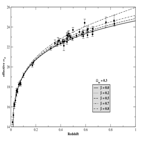
Figure 1: Hubble diagram for 16 low-redshift supernova and 38 high-redshift supernova from perlmutter . As indicated in the Figure, the curves correspond to a fixed value of $\Omega_{\rm{m}}=0.3$ and several values of $\beta$. For the sake of comparion the standard open case, $\beta=0$, is also shown (solid curve).

IV Constraints from current SNe Ia data

The apparent magnitude $m$ of a supernovae at a redshift $z$ is given by

$$m(z)={\cal M}+5\mbox{log}_{10}{\cal D}_{\mbox{{\scriptsize L}}}(\Omega_{\rm{m}},\beta,z)$$ (15)

where ${\cal M}=M-5\mbox{log}_{10}H_{0}+25$ is the “zero point magnitude”, $M$ is the absolute magnitude of the supernovae and ${\cal D}_{\mbox{{\scriptsize L}}}(\Omega_{\rm{m}},\beta,z)\equiv H_{o}d_{\mbox{{\scriptsize L}}}(\Omega_{\rm{m}},\beta,H_{o},z)$ is the dimensionless luminosity distance written as

$${\cal D}_{\mbox{{\scriptsize L}}}(\Omega_{\rm{m}},\beta,z) = (1+z)\times$$

$$\int_{(1+z)^{-1}}^{1}{dx\over x\left[1-\frac{\Omega_{\rm{m}}}{1-\beta}+\frac{\Omega_{\rm{m}}}{1-\beta}x^{-(1-3\beta)}\right]^{1/2}}.$$

The above expression can be integrated yielding

$${\cal D}_{\mbox{{\scriptsize L}}}(\Omega_{\rm{m}},\beta,z) = (1+z)\times$$

$$\frac{{\rm{sin}}\left[\delta\rm{sin}^{-1}\Delta_{1}-\delta\rm{sin}^{-1}\Delta_{2}\right]}{\left(\frac{\Omega_{\rm{m}}}{1-\beta}-1\right)^{\frac{1}{2}}},$$

where $\delta=\frac{2}{(1-3\beta)}$, $\Delta_{1}=(1-\frac{1-\beta}{\Omega_{\rm{m}}})^{{1\over 2}}$ and $\Delta_{2}=\Delta_{1}(1+z)^{-(\frac{1-3\beta}{2})}$. For $\frac{\Omega_{\rm{m}}}{1-\beta}=1$ or, equivalently, $k=0$ (flat case) the above equation reduces to

$${\cal D}_{\mbox{{\scriptsize L}}}(\beta,z)=\frac{2}{1-3\beta}\left[(1+z)-(1+z)^{\frac{1+3\beta}{2}}\right].$$ (18)

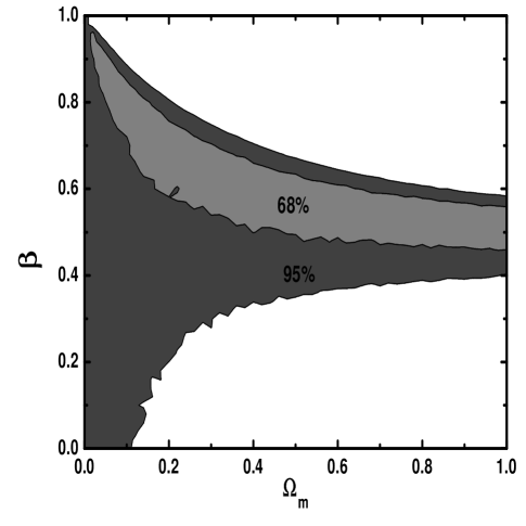
Figure 2: Confidence regions (68$\%$ and 95$\%$) in the $\Omega_{\rm{m}}-\beta$ plane provided by the SNe Ia data from Perlmutter et al. perlmutter .

In this analysis we consider the SNe Ia data set from the Supernova Cosmology Project (SCP) perlmutter . As noted in perlmutter , from the 60 supernova events, some are considered outliers so that we work with a total of 54 supernova (16 nearby ones and 38 at high redshifts). In order to determine the cosmological parameters $\Omega_{\rm{m}}$ and $\beta$, we use a $\chi^{2}$ minimization for a range of $\Omega_{\rm{m}}$ and $\beta$ spanning the interval [0,1] in steps of 0.02

$$\chi^{2}=\sum_{i=1}^{12}{\frac{\left[m(z_{i},{\cal M},\Omega_{\rm{m}},\beta)-m_{oi}\right]^{2}}{\sigma_{i}^{2}}},$$ (19)

where $m(z_{i},{\cal M},\Omega_{\rm{m}},\beta)$ is given by Eq. (6) and $m_{oi}$ is the observed values of the effective magnitude with errors $\sigma_{i}$ of the $i$th measurement in the sample. The “zero point magnitude” ${\cal M}$ is considered as a “nuisance” parameter so that we marginalize over it. 68$\%$ and 95$\%$ confidence regions are defined by the conventional two-parameters $\chi^{2}$ levels 2.30 and 6.17, respectively.

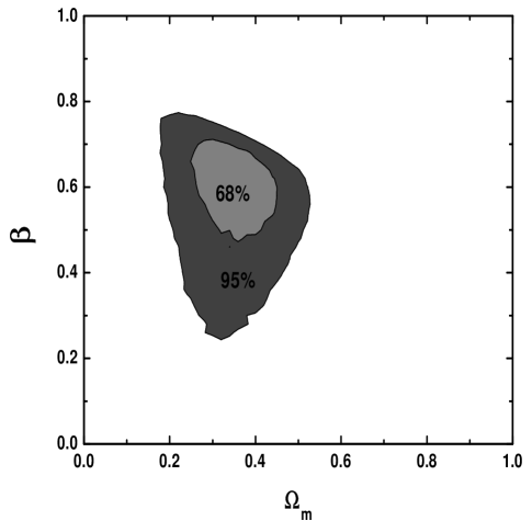
Figure 3: Confidence regions (68$\%$ and 95$\%$) in the $\Omega_{\rm{m}}-\beta$ plane provided by the SNe Ia data from Perlmutter et al. perlmutter by assuming a Gaussian prior on the matter density parameter $\Omega_{\rm{m}}=0.35\pm 0.07$.

In Fig. 1 we display the Hubble diagram for 16 low-redshift SNe Ia and 36 high-redshift SNe Ia from SCPperlmutter for $\Omega_{\rm{m}}=0.3$ and several values of $\beta$. For the sake of comparion the standard open case $\beta=0$ is also plotted. As has been shown recently mesa , a low-density decelerated model cannot be ruled out by SNe Ia data alone, although such a model is strongly deprived in the light of the recent CMB data. Figure 2 shows contours of constant likelihood (95$\%$ and 68$\%$) in the plane $\Omega_{\rm{m}}-\beta$. Note that the allowed range for both $\Omega_{\rm{m}}$ and $\beta$ is reasonably large, showing the impossibility of placing restrictive bounds on these scenarios from the current SNe Ia data without an additional constraint on the matter density parameter. The best fit model occurs for $\Omega_{\rm{m}}\simeq 1.0$ and $\beta\simeq 0.52$ with $\chi^{2}=62.83$ and 52 degrees of freedom. In Fig. 3 we show confidence regions in the $\Omega_{\rm{m}}-\beta$ plane by assuming a Gaussian prior on the matter density parameter, i.e., $\Omega_{\rm{m}}=0.35\pm 0.07$ ($95\%$ c.l.). Such a value is derived by combining the ratio of baryons to the total mass in clusters determined from X-ray and Sunyaev-Zeldovich measurements with the latest estimates of the baryon density $\Omega_{\rm{b}}=(0.020\pm 0.002)h^{-2}$ burles and the final value of the Hubble parameter obtained by the HST key Project $H_{o}=72\pm 8$ ${\rm{km.s^{-1}.Mpc^{-1}}}$ free . In this case the best fit model is strongly modified when compared with the previous analysis. It occurs for $\Omega_{\rm{m}}=0.34^{+0.14}_{-0.12}$ and $\beta=0.62^{+0.12}_{-0.24}$ (95$\%$ c.l.) with $\chi^{2}=63.44$. These results agree with the limits on the decaying parameter $\beta$ from measurements of the angular size of high-redshift radio sources. This latter analysis indicates $\beta\simeq 0.6$ while the current estimates for the age of the Universe provides $\beta\geq 0.25$ jailson .

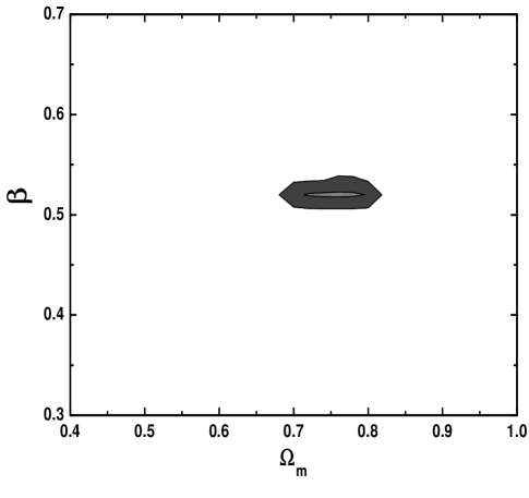
Figure 4: Simulation of the confidence limits from a SNAP-type data set generated by assuming that we live in a flat $\Lambda$CDM universe with $\Omega_{\rm{m}}=0.28$ and $\Omega_{\Lambda}=0.72$. The dark shaded region corresponds to 95$\%$ c.l. while the brighter shaded region corresponds to 68$\%$ c.l.

V Constraints from future SNe data

Let us now discuss the constraints on deflationary $\Lambda(t)$ cosmologies that may be expected from future SNe Ia data. Such data may be provided by the proposed SNAP satelite, a two-meter space telescope dedicated to SNe Ia observations on a wide range of redshifts snap . In this Section we investigate the limits on the decaying rate $\beta$ based on one year of SNAP data. To this end, we follow Goliath et al. goli and assume 2000 supernova in the redshift interval $z\in[0,1.2]$ and an additional of 100 supernova at higher redshifts, $z\in[1.2,1.7]$. Each interval has been binned with $\Delta z=0.05$. The statistical error in magnitude, including the estimated measurement error of the distance modulus and the dispersion in the distance modulus due to dispersion in galaxy redshift, is assumed to be $\Delta m=0.15$ mag. The supernova data set was generated by assuming that we live in a flat $\Lambda$CDM universe with $\Omega_{\rm{m}}=0.28$ and $\Omega_{\Lambda}=0.72$.

Figure 4 shows the corresponding confidence regions for the $\Omega_{\rm{m}}-\beta$ plane from this simulated supernova data et. In comparison with Figs. 2 and 3, we see that the allowed parameter space is strongly restricted by the SNAP data. In particular, the statistical uncertainty on the $\beta$ parameter reduces from ${}^{+0.12}_{-0.24}$ (by assuming a prior knowledge on $\Omega_{\rm{m}}$) to $\sim{0.015}$. This result shows that future SNe Ia data will provide much tighter constraints on deflationary cosmologies or, possibly, on any kind of decaying $\Lambda(t)$ cosmologies, than do the current observations. Naturally, only with a more general analysis, a joint investigation involving different classes of cosmological tests, it will be possible to delimit the $\Omega_{\rm{m}}-\beta$ plane more precisely, as well as to test more properly the consistency of these scenarios. Such an analysis will appear in a forthcoming communication alc .

VI Conclusion

The results of observational cosmology in the last years have opened up an unprecented opportunity to test the veracity of a number of cosmological scenarios. The most remarkable finding among these results cames from distance meaurements of SNe Ia at intermediary redshifts that suggest that the expansion of the Universe is speeding up, not slowing down. In this work, we investigated the observational constraints on a particular class of deflationary cosmologies provided by the current and future SNe Ia data. We showed that the supernova data alone cannot place restrictive constraints on the decaying parameter $\beta$ unless a prior knowledge of the matter density parameter is introduced. In this case, by assuming the gaussian prior $\Omega_{\rm{m}}=0.35\pm 0.07$ we found $\beta=0.62^{+0.12}_{-0.24}$ at 95$\%$ c.l. Such a result is in agreement with recent estimates of the $\beta$ parameter from measurements of the angular size of high-redshift radio sources and age estimates of globular clusters jailson . By simulating one year of SNAP data we also found that very restrictive limits will be placed on such cosmologies, with error estimates on the decaying $\beta$ parameter of the order of $\pm 0.02$.

- (1) S. Perlmutter et al., Astrophys. J. 517, 565 (1999).
- (2) A. Riess et al., Astron. J. 116, 1009 (1998).
- (3) P. de Bernardis et al., Nature 404, 955 (2000); A. E. Lange et al., Phys. Rev. D63, 042001 (2001); A. Balbi et al., Astrophys. J. 545, L1; (2000).
- (4) R. G. Calberg et al., Astrophys. J. 462, 32 (1996); A. Dekel, D. Burstein and S. White S., In Critical Dialogues in Cosmology, edited by N. Turok World Scientific, Singapore (1997).
- (5) E. Carretta et al., Astrophys. J. 533, 215 (2000); L. M. Krauss and B. Chaboyer, astro-ph/0111597; M. Rengel, J. Mateu and G. Bruzual, IAU Symp. 207, Extragalactic Star Clusters, Eds. E. Grebel, D. Geisler, D Minnite (in Press), astro-ph/0106211 (2002).
- (6) J. Dunlop, In The Most Distant Radio Galaxies, ed. H. J. A. Rottgering, P. Best, and M. D. Lehnert, Dordrecht: Kluwer, 71 (1998); L. M. Krauss, Astrophys. J. 480, 486 (1997); J. S. Alcaniz and J. A. S. Lima, Astrophys. J. 521, L87 (1999).
- (7) S. Weinberg, Rev. Mod. Phys. 61, 1 (1989); V. Sahni and A. A. Starobinsky, Int. J. Mod. Phys. D9, 373 (2000).
- (8) M. Özer and M. O. Taha Phys. Lett. B171, 363 (1986); Nucl. Phys. B287, 776 (1987).
- (9) O. Bertolami, Nuovo Cimento, B93, 36 (1986); K. Freese, F. C. Adams, J. A. Frieman and E. Mottola, Nucl. Phys. B287, 797 (1987); W. Chen and Y.-S. Wu, Phys. Rev. D41, 695 (1990); J. C. Carvalho, J. A. S. Lima and I. Waga, Phys. Rev. D46 2404 (1992); J. M. Salim and I. Waga, Class. Quant, Grav. 10, 1767 (1993); I. Waga, Astrophys. J. 414, 436 (1993); J. A. S. Lima and J. C. Carvalho, Gen. Rel. Grav. 29, 909 (1994); O. Bertolami and P. J. Martins, Phys. Rev. D61, 064007 (2000); R. G. Vishwakarma, Gen. Rel. Grav. 33, 1973 (2001).
- (10) F. M. Overduin and F. I. Cooperstock, Phys. Rev. D58, 043506 (1998).
- (11) J. A. S Lima and J. M. F. Maia, Phys. Rev. D49, 5597 (1994).
- (12) J. A. S. Lima and M. Trodden, Phys. Rev. D53, 4280 (1996).
- (13) A. Berera and L. Z. Fang, Phys. Rev. Lett. 74, 1912 (1995); A. Berera, Phys. Rev. Lett. 75, 3218 (1995); Phys. Rev. D54, 2519 (1996); H. P. de Oliveira and R. O. Ramos, Phys. Rev. D 57, 741 (1998); A. N. Taylor and A. Berera, Phys. Rev. D 62, 083517 (2000).
- (14) J. V. Cunha, J. S. Alcaniz and J. A. S. Lima, Phys. Rev. 66, 023520 (2002).
- (15) E. Gunzig, R. Maartens and A. Nesteruk, Class. Quant. Grav. 15, 923 (1998).
- (16) R. Maartens, D. R.Taylor and N. Roussos, Phys. Rev.D52, 3358 (1995).
- (17) W. Zimdahl, Phys. Rev. D61, 083511 (2000); W. Zimdahl and A. B. Balakin, Phys. Rev. D63, 023507 (2001).
- (18) J. M. F. Maia and J. A. S. Lima, Phys. Rev. D65, 083513 (2002).
- (19) J. V. Cunha, J. A. S. Lima and N. Pires, Astron. and Astrop. 390, 809 (2002).
- (20) L. F. Bloomfield Torres and I. Waga, Mon. Not. R. Astron. Soc. 279, 712 (1996).
- (21) R. G. Vishwakarma, Class. Quant. Grav. 18, 1159 (2001).
- (22) See http://snap.lbl.gov.
- (23) D. Huterer and M. S. Turner, Phys. Rev. D60, 081301 (1999); T. D. Saini, S. Raychaudhuri, V. Sahni and A. A. Starobinsky, Phys. Rev. Lett. 85, 1162 (2000); P. Astier astro-ph/0008306; J. Weller and A. Albrecht, Phys. Rev. Lett. 86, 1939 (2000); Phys. Rev. 65, 103512 (2002).
- (24) E. W. Kolb, Astrophys. J. 344, 543 (1989)
- (25) A. P. Billyard and A. A. Coley, Phys. Rev. D 61, 083503 (2000); L. Amendola, Phys. Rev. D 62, 043511 (2000); W. Zimdahl, D. Pav n and L. P. Chimento, Phys. Lett. B 521, 133 (2001); D. Tocchini-Valentini and L. Amendola, Phys. Rev. D 65 (2002) 063508; W. Zimdahl, A. B. Balakin, D. J. Schwarz and D. Pavon, astro-ph/0210204
- (26) A. Meszaros, astro-ph/0207558.
- (27) S. Burles, K. M. Nollett and M. S. Turner, Astrophys. J. 552, L1 (2001).
- (28) W. L. Freedman et al., Astrophys. J. 553, 47 (2001).
- (29) M. Goliath, R. Amanullah, P. Astier, A. Goobar and R. Pain, Astro. Astrop. 380, 6 (2001)
- (30) J. S. Alcaniz, in preparation.