Disk Accretion Flow Driven by Large-Scale Magnetic Fields: Solutions with Constant Specific Energy

Abstract

We study the dynamical evolution of a stationary, axisymmetric, and perfectly conducting cold accretion disk containing a large-scale magnetic field around a Kerr black hole, trying to understand the relation between accretion and the transportation of angular momentum and energy. A one-dimensional radial momentum equation is derived near the equatorial plane, which has one intrinsic singularity at the fast critical point. We solve the radial momentum equation for solutions corresponding to an accretion flow that starts from a subsonic state at infinity, smoothly passes the fast critical point, then supersonically falls into the horizon of the black hole. The solutions always have the following features: 1) The specific energy of fluid particles remains constant but the specific angular momentum is effectively removed by the magnetic field. 2) At large radii, where the disk motion is dominantly rotational, the energy density of the magnetic field is equipartitioned with the rotational energy density of the disk. 3) Inside the fast critical point, where radial motion becomes important, the ratio of the electromagnetic energy density to the kinetic energy density drops quickly. The results indicate that: 1) Disk accretion does not necessarily imply energy dissipation since magnetic fields do not have to transport or dissipate a lot of energy as they effectively transport angular momentum. 2) When resistivity is small, the large-scale magnetic field is amplified by the shearing rotation of the disk until the magnetic energy density is equipartitioned with the rotational energy density, ending up with a geometrically thick disk. This is in contrast with the evolution of small-scale magnetic fields where if the resistivity is nonzero the magnetic energy density is likely to be equipartitioned with the kinetic energy density associated with local random motions (e.g., turbulence), making a thin Keplerian disk possible.

I Introduction

Accretion onto a gravitating object is believed to be a principal energy source for powering many astrophysical systems, including active galactic nuclei (AGN), quasars, and some types of stellar binaries fra02 . Since accreting gases far from the central object typically have sufficiently large specific angular momentum compared to a particle moving on a circular orbit around and near the central object, the formation of an accretion disk is unavoidable. To accrete onto the central object and release gravitational energy, gases at large distance must lose a lot of angular momentum. It is usually assumed that some kind of viscosity slowly operates in a disk to transport angular momentum outward and dissipate energy, so that to a very good approximation in the disk region particles move on circular orbits with a small radial velocity superposed.

The simplest stationary and axisymmetric model of accretion disk is a geometrically thin Keplerian disk, where it is assumed that in the disk region the gravity of the central object is approximately balanced by the centrifugal force so that disk particles move approximately on Keplerian circular orbits sha73 ; nov73 ; Page & Thorne (1974). Then, at each radius, the specific angular momentum and the specific energy of disk particles are given by that of a test particle moving on the Keplerian circular orbit at that radius. When the central object is a black hole, the Keplerian disk has an inner boundary at the marginally stable circular orbit, inside which the gravity is too strong to be balanced by the centrifugal force bar72 ; nov73 ; Page & Thorne (1974). The total efficiency of converting mass into energy is defined by

$$\varepsilon\equiv\frac{\delta{\cal E}}{\delta M}\;,$$ (1)

where $\delta{\cal E}$ is the total released energy during the process of accretion, $\delta M$ is the corresponding accreted mass . Then, the total efficiency of a Keplerian disk around a Kerr black hole is given by the difference between the specific energy at infinity ($E_{\infty}=1$) and the specific energy on the marginally stable circular orbit ($E_{\rm ms}$)

$$\varepsilon_{\rm Keplerian}=1-E_{\rm ms}\;.$$ (2)

Thin Keplerian disks correspond to the most efficient case of releasing the gravitational energy of an accretion flow. For a thin Keplerian disk around a Schwarzschild black hole, the total efficiency is $\varepsilon_{\rm Keplerian}\approx 0.06$. For a thin Keplerian disk around a “canonical” Kerr black hole of specific spinning angular momentum $a=0.998M$, where $M$ is the mass of the black hole, the total efficiency is $\varepsilon_{\rm Keplerian}\approx 0.32$ when the effect of radiation capture is considered tho74 . These efficiencies of converting mass into energy are indeed much higher than nuclear fusion, the latter is $\approx 0.007$ for hydrogen. The released gravitational energy in a thin Keplerian disk is assumed to be efficiently dissipated by the internal viscosity and instantly radiated away from the surfaces of the disk.

Though the model of geometrically thin and optically thick Keplerian accretion disks is supported by the appearance of Big Blue Bump in the spectra of all bright AGN (shi78 ; kor99 ; kis03 and references therein), it is challenged by the observational fact that most nearby galactic nuclei are much less active—sometimes not active at all (nar02 and references therein). These objects have luminosities that are lower than what a thin Keplerian disk model usually predicts by many orders of magnitudes. In order to interpret this phenomenon, different disk models are proposed where either the radiative efficiency is assumed to be low so that the released gravitational energy is converted into entropy and internal energy trapped in the flow and carried into the central black hole by the flow, or the mass accretion rate is assumed to be low and most of the released gravitational energy is carried away by a mass outflow nar94 ; bla99b ; sto99 ; nar00 ; qua00 ; igu03 . These alternative models are summarized by Blandford bla99a and Narayan nar02 . Though they predict a different disk luminosity, these models are in common with the thin Keplerian disk in the following aspect: the mechanical energy (= gravitational potential energy + kinetic energy) of the disk flow is efficiently converted into other forms of energy.

In the theory aspect, the proposed disk viscosity is poorly understood. Investigations on the magnetohydrodynamics (MHD) in a differentially rotating disk suggest that magnetic fields may play the role of disk viscosity (bal98 ; bla02 and references therein). Due to the existence of magnetorotational instability, MHD turbulence is easily generated in a differentially rotating disk, which effectively transports angular momentum outward and drives accretion (bal91 ; sto96 ; haw96 ; haw00 ; haw02 and references therein). However, very few models of disk radiation are based on these ideas, and generally angular momentum transport is treated through a parameterized viscous stress—the so-called $\alpha$-viscosity following Shakura & Sunyaev sha73 ; kor99 . This is because of the fact that though it is well established that magnetic fields effectively transport angular momentum and drive accretion, it is far from clear how magnetic fields transport and dissipate energy in the meantime. Numerical simulations are a powerful tool for studying the nonlinear evolution of magnetic fields. However, numerical simulations usually have large numerical dissipation due to finite spatial resolutions, which makes energy transportation and dissipation cannot be accurately studied with current numerical simulations haw95 ; ryu95 ; bal98 ; bla02 . Therefore, our current understanding on how magnetic fields transport and dissipate energy is much worse than our understanding on how magnetic fields transport angular momentum.

In this paper we ask and try to answer the following question: Do magnetic fields transport or dissipate energy as efficiently as they transport angular momentum? Or, more precisely, Do magnetic fields have to transport or dissipate a lot of energy as they efficiently transport angular momentum in a disk accretion flow?

To answer this question (or, to get some insight into the answer), we use an analytical model to study the dynamical effects of magnetic fields in an accretion disk around a Kerr black hole. The disk is assumed to be stationary, axisymmetric, perfectly conducting, and contain a large-scale magnetic field . Both the magnetic field and the velocity field of the disk fluid have only radial and azimuthal components in a small neighborhood of the disk central plane $\theta=\pi/2$, where $\theta$ is the polar angle from the symmetry axis of the black hole. In other words, near the central plane of the disk, each magnetic field line lies on a surface of constant $\theta$, and the same is true for each fluid stream line. (Similar approach is usually used to study the inflow/outflow problem associated with a low density magnetosphere around a black hole or neutron star, see cam86 ; cam86a ; tak90 ; hir92 ; dai02 ; tak02 , and pun01 for a review.) For simplicity, we neglect the thermal pressure in the disk by assuming that the accretion flow is cold. Then, making use of the conservation of rest mass, energy, and angular momentum, Maxwell’s equations and dynamical equations are reduced to a set of one-dimensional equations with radius $r$ as the only variable. We will self-consistently solve these equations, to look for the relation between accretion and the transportation of angular momentum and energy.

Gammie gam99 has used the model to study the flow on the equatorial plane in the plunging region between the inner boundary of the disk and the horizon of the black hole. Gammie’s model is further explored by Li li03 and tested with numerical simulations by De Villiers & Hawley vil02 . In this paper we extend the model into the disk region, and into a small neighborhood of the equatorial plane. This extension allows us to investigate a disk accretion flow driven by magnetic fields from a global view: from the subsonic far outer disk region down to the supersonic deep plunging region . We emphasize that such a model can only be applied to a large-scale and ordered magnetic field. For small-scale and chaotic magnetic fields, the gradient of the magnetic field is important, making the solutions invalid when even a small nonzero resistivity is introduced (see Sec. VI for detail).

The paper is organized as follows: In Sec. II we exactly solve Maxwell’s equations for the model outlined above. In Sec. III we write down the equations for the conservation of rest mass, the conservation of angular momentum, and the conservation of energy. We show that the solutions always correspond to an accretion flow with constant specific energy when reasonable boundary conditions at infinity are satisfied. Then we derive a one-dimensional radial momentum equation corresponding to the magnetized disk accretion flow. In Sec. IV we discuss the analytical properties of the radial momentum equation, the solutions on the horizon of the black hole, and the asymptotic solutions at infinity. We show that the fast critical point is the only intrinsic singularity in the radial momentum equation. In Sec. V we present some explicit solutions representing a magnetized disk flow with constant specific energy accreting from infinity onto a central black hole. In Sec. VI we discuss the effect of finite resistivity and compare the evolution of large-scale magnetic fields to that of small-scale magnetic fields. In Sec. VII we summarize the results and draw our conclusions.

In Appendix A we make some effort to generalize our results to more general and more complicated models. In Appendix B we present the Newtonian limit of our solutions.

II Solutions to Maxwell’s Equations

We assume that the background spacetime is described by the metric of a Kerr black hole of mass $M$ and specific angular momentum $a$, where $-M\leq a\leq M$. In Boyer-Lindquist coordinates $(t,r,\theta,\phi)$, the metric of a Kerr black hole is given by mis73 ; wal84

$$ds^{2}=-\left(1-\frac{2Mr}{\Sigma}\right)dt^{2}-\frac{4Mar}{\Sigma}\,\sin^{2}\theta\,dtd\phi+\frac{\Sigma}{\Delta}\,dr^{2}+\Sigma\,d\theta^{2}+\frac{\Lambda\sin^{2}\theta}{\Sigma}\,d\phi^{2}\;,$$ (3)

where

$$\Delta\equiv r^{2}-2Mr+a^{2}\;,\hskip 28.45274pt\Sigma\equiv r^{2}+a^{2}\cos^{2}\theta\;,\hskip 28.45274pt\Lambda\equiv(r^{2}+a^{2})^{2}-\Delta a^{2}\sin^{2}\theta\;.$$ (4)

The radius of the outer event horizon is at $r_{\rm H}=M+\left(M^{2}-a^{2}\right)^{1/2}$.

As stated in the Introduction, we focus on solutions in a small neighborhood of the equatorial plane defined by $\cos^{2}\theta\ll 1$. Then, to the first order of $\cos\theta$ , the metric does not depend on $\theta$ and is given by

$$ds^{2}=-\left(1-\frac{2M}{r}\right)dt^{2}-\frac{4Ma}{r}\,dtd\phi+\frac{r^{2}}{\Delta}\,dr^{2}+r^{2}d\theta^{2}+\frac{A}{r^{2}}\,d\phi^{2}\;,$$ (5)

where $A\equiv\Lambda(\theta=\pi/2)$.

Assuming that the disk fluid is perfectly conducting so that magnetic field lines are frozen to the fluid. Then, in terms of coordinate components, the Maxwell equations that we need to solve are reduced to lic67 ; li03

$$\frac{1}{\sqrt{-g}}\frac{\partial}{\partial x^{\alpha}}\left[\sqrt{-g}\left(u^{\alpha}B^{\beta}-u^{\beta}B^{\alpha}\right)\right]=0\;,$$ (6)

where $x^{\alpha}=(t,r,\theta,\phi)$, $\sqrt{-g}=r^{2}$ (to the first order of $\cos\theta$), $u^{\alpha}$ is the four-velocity of the fluid, and $B^{\alpha}$ is the magnetic field measured by an observer comoving with the fluid. (The electric field measured by an observer comoving with a perfectly conducting fluid is zero.)

We assume that in the small neighborhood of the equatorial plane we have

$$u^{\theta}=0\;,\hskip 28.45274ptB^{\theta}=0\;,$$ (7)

i.e., each line of velocity or magnetic field lies on a surface of $\theta=\mbox{constant}$. Equation (7) implies that

$$\frac{\partial u^{\theta}}{\partial\theta}=0\;,\hskip 28.45274pt\frac{\partial B^{\theta}}{\partial\theta}=0\;,$$ (8)

in the same neighborhood. Then, for stationary and axisymmetric solutions with $\partial/\partial t=\partial/\partial\phi=0$, the Maxwell equation (6) is reduced to

$$\frac{\partial}{\partial r}\left[r^{2}(u^{r}B^{\beta}-u^{\beta}B^{r})\right]=0\;.$$ (9)

By definition, $B^{a}$ satisfies $u_{a}B^{a}=0$. Then, making use of $u_{a}u^{a}=-1$, we can solve for $B^{r}$, $B^{\phi}$, and $B^{t}$ from Eq. (9). The results are

$$B^{r} = \frac{1}{r^{2}}(-C_{0}u_{t}+\Psi u_{\phi})\;,$$ (10)

$$B^{\phi} = \frac{1}{r^{2}u^{r}}[-C_{0}u_{t}u^{\phi}+(1+u_{\phi}u^{\phi})\Psi]\;,$$ (11)

$$B^{t} = \frac{1}{r^{2}u^{r}}[-(1+u_{t}u^{t})C_{0}+u_{\phi}u^{t}\Psi]\;,$$ (12)

where $C_{0}$ and $\Psi$ are constants.

The electromagnetic field tensor corresponding the solutions given by Eqs. (10)–(12) is

$$F_{ab}=\epsilon_{abcd}u^{c}B^{d}=-2\Psi\,dt_{[a}d\theta_{b]}+\frac{2}{u^{r}}\left(C_{0}u^{\phi}+\Psi u^{t}\right)dr_{[a}d\theta_{b]}+2C_{0}\,d\theta_{[a}d\phi_{b]}\;,$$ (13)

where $\epsilon_{abcd}$ is the totally antisymmetric tensor of the volume element that is associated with the metric wal84 , the brackets “[ ]” denote antisymmetrization. Gammie gam99 obtained the same solution for $F_{ab}$ by directly solving the Maxwell equation $\nabla_{[a}F_{bc]}=0$.

It is useful to have a look at the magnetic field and the electric field measured by an observer in the locally nonrotating frame (LNRF observer, see bar72 ) in the equatorial plane, whose four-velocity is $U^{a}=\chi^{-1}\left[\left(\partial/\partial t\right)^{a}+\omega\left(\partial/\partial\phi\right)^{a}\right]$, where $\chi\equiv\left(r^{2}\Delta/A\right)^{1/2}$ and $\omega\equiv 2Mar/A$ are respectively the lapse function (i.e., the redshift factor) and the frame dragging angular velocity. From the electromagnetic field tensor in Eq. (13), we can calculate the magnetic field and the electric field measured by a LNRF observer

$$B^{\prime a} \equiv -\frac{1}{2}\epsilon^{a}_{~{}bcd}U^{b}F^{cd}=\frac{\chi C_{0}}{r^{2}}\left(\frac{\partial}{\partial r}\right)^{a}+\frac{\chi}{r^{2}u^{r}}\left(C_{0}u^{\phi}+\Psi u^{t}\right)\left(\frac{\partial}{\partial\phi}\right)^{a}\;,$$ (14)

$$E^{\prime a} \equiv F^{a}_{~{}b}U^{b}=\frac{1}{\chi r^{2}}(C_{0}\omega+\Psi)\left(\frac{\partial}{\partial\theta}\right)^{a}\;.$$ (15)

Therefore, the constant $C_{0}$ measures the flux of the radial magnetic field, and the constant $\Psi$ is related to the electric field measured by a LNRF observer and thus measures the direction of the magnetic field relative to the fluid motion li03 .

Equation (10) can be rewritten as $\Psi=u_{\phi}^{-1}(r^{2}B^{r}+C_{0}u_{t})$. For a Keplerian disk we have $u_{t}=-1$ and $u_{\phi}\propto r^{1/2}$ as $r\rightarrow\infty$. If generally we assume that $u_{t}$ and $r^{2}B^{r}$ are bounded but $u_{\phi}$ is unbounded as $r\rightarrow\infty$, then we must have

$$\Psi=0\;,\hskip 17.07182pt\mbox{i.e.,}\hskip 17.07182pt\frac{B^{r}}{B^{\phi}}=\frac{u^{r}}{u^{\phi}}\;.$$ (16)

We note that it is not obvious that $r^{2}B^{r}$ must be finite, since the magnetic flux across a circle of a radius $r$ is $\propto r^{2}B^{\prime r}/\chi$, not $r^{2}B^{r}$. Stronger justifications for the validity of Eq. (16) are given in the next section where dynamical equations are discussed.

From Eqs. (10) and (11) we have

$$k\equiv 1-\frac{B^{\phi}u^{r}}{B^{r}u^{\phi}}=-\frac{\Psi}{\left(-C_{0}u_{t}+\Psi u_{\phi}\right)u^{\phi}}\;.$$ (17)

Because of the appearance of $u^{\phi}$ in the denominator on the right-hand side, which generally quickly decreases with radius (e.g., $u^{\phi}/u^{t}\propto r^{-3/2}$ for a Keplerian disk), $|k|$ grows quickly as $r$ increases, if $\Psi\neq 0$. This means that, if at a large radius $k$ is $\sim 1$, then $k$ quickly approaches zero as $r$ decreases.

As an example, assuming that at $r=r_{0}\gg r_{\rm H}$ we have $k=k_{0}\sim 1$ (which is true if $B^{r}\sim rB^{\phi}$ and $|u^{r}/ru^{\phi}|\ll 1$ at $r=r_{0}$), then by Eq. (17) we have

$$\Omega_{\Psi}\equiv-\frac{\Psi}{C_{0}}=\left.-\frac{k_{0}u_{t}u^{\phi}}{1+k_{0}u_{\phi}u^{\phi}}\right|_{r=r_{0}}\approx k_{0}\Omega_{0}\;,$$ (18)

where $\Omega_{0}\equiv\left(u^{\phi}/u^{t}\right)_{r=r_{0}}$ is the angular velocity of the disk at $r=r_{0}\,$. In the last step we have used the fact that $u_{t}\approx-u^{t}\approx-1$ and $u_{\phi}u^{\phi}\sim M/r\ll 1$ at $r=r_{0}$ . Substitute Eq. (18) into Eq. (17), we then obtain

$$k\approx-\frac{k_{0}\Omega_{0}}{\left(u_{t}+k_{0}\Omega_{0}u_{\phi}\right)u^{\phi}}$$

at any radius $r$. For $r\ll r_{0}$ in a Keplerian-type disk we have

$$|k|\approx\left|\frac{k_{0}\Omega_{0}}{u_{t}u^{\phi}}\right|\sim\left(\frac{r}{r_{0}}\right)^{3/2}\ll 1\;,$$ (19)

since $u_{0}^{\phi}u_{\phi}\sim(M/r_{0})(r/r_{0})^{1/2}\ll 1$ and $u_{t}\sim-1$.

When Eq. (16) is satisfied, from Eq. (15) we have $E^{\prime a}=\left(C_{0}\omega/\chi r^{2}\right)(\partial/\partial\theta)^{a}$. Then, for a Schwarzschild black hole (i.e., $a=\omega=0$), we have $E^{\prime a}=0$, i.e., the magnetic field is parallel to the velocity field as seen by a local static observer (equivalent to a LNRF observer for a Kerr black hole). For a Kerr black hole with $a\neq 0$, the electric field measured by a LNRF observer is nonzero. However, the electric field decays quickly with increasing $r$: $E^{\prime}_{a}E^{\prime a}\propto r^{-8}$ for $r\gg r_{\rm H}$. Therefore, for a Kerr black hole, to a good approximation the magnetic field is also parallel to the velocity field in a LNRF, unless in the region close to the horizon of the black hole. Therefore, when Eq. (16) is satisfied, we say that the magnetic field is parallel to the velocity field; or equivalently, the magnetic field lines are aligned with the fluid motion. But it must be kept in mind that this statement is not very accurate for the case of a Kerr black hole according to the above discussion.

Equation (19) indicates that after the disk flow settles into the stationary and axisymmetric state the magnetic field and the velocity field tend to be aligned with each other if they are not so initially.

In the next section we will see that a magnetic field satisfying Eq. (16) has a very interesting feature: it does not change the specific energy of fluid particles though it affects the specific angular momentum. Physically this is caused by the fact that the electromagnetic force produced by the magnetic field satisfying Eq. (16) is always perpendicular to the velocity of the fluid.

III Derivation of the Radial Momentum Equation

For a cold and perfectly conducting magnetized fluid the total stress-energy tensor is given by $T^{ab}=\rho_{\rm m}u^{a}u^{b}+T_{\rm EM}^{ab}$, where $\rho_{\rm m}$ is the mass-energy density of the fluid matter as measured by an observer comoving with the fluid, $T_{\rm EM}^{ab}$ is the stress-energy tensor of the magnetic field lic67 ; li03

$$T_{\rm EM}^{ab}=\frac{1}{4\pi}B^{2}u^{a}u^{b}+\frac{1}{8\pi}B^{2}g^{ab}-\frac{1}{4\pi}B^{a}B^{b}\;.$$ (20)

By Einstein’s equation, the dynamical equations of the magnetized fluid are given by mis73 ; wal84

$$\nabla_{a}T^{ab}=0\;.$$ (21)

III.1 Conservation laws

A number of conservation laws can be derived from Eq. (21) lic67 ; bek78 ; wal84 ; li03 . The contraction of $u_{b}$ with Eq. (21) leads to the conservation of rest mass (also called the continuity equation): $\nabla_{a}\left(\rho_{\rm m}u^{a}\right)=0$ . The contraction of $(\partial/\partial\phi)^{a}$ with Eq. (21) leads to the conservation of angular momentum: $\nabla_{a}T_{\phi}^{~{}a}=0$ . The contraction of $(\partial/\partial t)^{a}$ with Eq. (21) leads to the conservation of energy: $\nabla_{a}T_{t}^{~{}a}=0$ . [Note that $(\partial/\partial t)^{a}$ and $(\partial/\partial\phi)^{a}$ are Killing vectors of a Kerr spacetime.]

Because of Eqs. (7) and (8), for stationary and axisymmetric solutions in the small neighborhood of the disk central plane, the above conservation equations are simplified to one-dimensional ordinary differential equations li03

$$\frac{d}{dr}\left(r^{2}\rho_{\rm m}u^{r}\right) = 0\;;$$ (22)

$$\frac{d}{dr}\left[r^{2}\left(\rho_{\rm m}u_{\phi}u^{r}+T_{{\rm EM},\phi}^{~{}~{}~{}~{}~{}r}\right)\right] = 0\;;$$ (23)

$$\frac{d}{dr}\left[r^{2}\left(\rho_{\rm m}u_{t}u^{r}+T_{{\rm EM},t}^{~{}~{}~{}~{}~{}r}\right)\right] = 0\;;$$ (24)

respectively.

Substituting the solutions (10)–(12) into Eq. (20), we obtain

$$T_{{\rm EM},\phi}^{~{}~{}~{}~{}~{}r} = \frac{1}{4\pi}\left(B^{2}u_{\phi}u^{r}-B_{\phi}B^{r}\right)=-\frac{C_{0}\Delta}{4\pi r^{4}u^{r}}\left(C_{0}u^{\phi}+\Psi u^{t}\right)\;,\hskip 17.07182pt$$ (25)

$$T_{{\rm EM},t}^{~{}~{}~{}~{}~{}r} = \frac{1}{4\pi}\left(B^{2}u_{t}u^{r}-B_{t}B^{r}\right)=-\Omega_{\Psi}T_{{\rm EM},\phi}^{~{}~{}~{}~{}~{}r}\;,$$ (26)

where $\Omega_{\Psi}$ is defined by Eq. (18). (Though based on the arguments in Sec. II we expect $\Psi=0$ in a stationary state, in this section we keep $\Psi$ in the derived formulas to make the formulas as general as possible.)

The solution to Eq. (22) is

$$\rho_{\rm m}=\frac{F_{\rm m}}{4\pi r^{2}u^{r}}\;,$$ (27)

where $F_{\rm m}$ is the constant of radial mass flux. From Eqs. (10)–(12), at large radii where $r\gg M$, $u_{t}\approx-u^{t}\approx-1$, $u^{r}\approx 0$, $u^{\phi}\approx 0$, and $u_{\phi}$ is unbounded, we have $B^{2}=B_{a}B^{a}\approx\Psi^{2}/r^{2}\left(u^{r}\right)^{2}$, if $\Psi\neq 0$ and $u_{\phi}^{2}/r^{2}\ll 1$ (e.g., $u_{\phi}^{2}/r^{2}\approx M/r$ for a Keplerian disk). Then

$$\frac{B^{2}}{4\pi\rho_{\rm m}}\approx\frac{\Psi^{2}}{F_{\rm m}u^{r}}\propto\frac{1}{-u^{r}}\;,$$ (28)

as $r\rightarrow\infty$. Equation (28) implies that if $\Psi\neq 0$, at sufficiently large radii the magnetic field must be so strong that $B^{2}/4\pi\gg\rho_{\rm m}$. In order to prevent this to happen, $\Psi$ must be zero. This provides a strong support for Eq. (16).

Making use of Eqs. (25)–(27), we can integrate Eqs. (23) and (24) to obtain

$$u_{\phi}+\frac{c_{0}^{2}\Delta}{r^{2}u^{r}}\left(u^{\phi}-\Omega_{\Psi}u^{t}\right)=-f_{\rm L}\;,$$ (29)

$$u_{t}-\Omega_{\Psi}\frac{c_{0}^{2}\Delta}{r^{2}u^{r}}\left(u^{\phi}-\Omega_{\Psi}u^{t}\right)=f_{\rm E}\;,$$ (30)

where

$$c_{0}\equiv\frac{C_{0}}{\sqrt{-F_{\rm m}}}\;,\hskip 28.45274ptf_{\rm L}\equiv\frac{F_{\rm L}}{-F_{\rm m}}\;,\hskip 28.45274ptf_{\rm E}\equiv\frac{F_{\rm E}}{-F_{\rm m}}\;,$$ (31)

$F_{\rm L}=4\pi r^{2}T_{\phi}^{~{}r}$ and $F_{\rm E}=-4\pi r^{2}T_{t}^{~{}r}$ are the constants of radial angular momentum flux and radial energy flux, respectively. The dynamical equations (29) and (30) do not depend on the sign of $c_{0}$. Without loss of generality, henceforth we assume that $c_{0}>0\,$.

From Eqs. (29) and (30) we have

$$E-\Omega_{\Psi}L=-f_{\rm E}+\Omega_{\Psi}f_{\rm L}\;,$$ (32)

where $E=-u_{t}$ is the specific energy, $L=u_{\phi}$ is the specific angular momentum of fluid particles. Since $f_{\rm E}$, $f_{\rm L}$, and $\Omega_{\Psi}$ are constants, Eq. (32) immediately implies that the specific energy $E$ must be constant when $\Psi=0$ (i.e., $\Omega_{\Psi}=0$), and the specific angular momentum $L$ must be constant when $C_{0}=0$ but $\Psi\neq 0$ (i.e., $\left|\Omega_{\Psi}\right|=\infty$).

The variation of Eq. (32) leads to

$$\delta E=\Omega_{\Psi}\delta L\;.$$ (33)

Obviously, $\Omega_{\Psi}$ cannot be negative if we want $\delta E/\delta L\geq 0\,$, i.e., angular momentum and energy propagate in the same direction.

If the outer boundary of the disk flow is at $r=\infty$ and the specific angular momentum $L$ is unbounded at $r=\infty$, then we have $\delta L=L(r=\infty)-L(r)=\infty$ for any finite $r$. Generally $E$ is positive and bounded at $r=\infty$ and $E$ must be positive outside the ergosphere of a Kerr black hole. Hence, $\delta E=E(r=\infty)-E(r)$ must be finite for $r>2M$. Then, by Eq. (33), this can be true if and only if $\Omega_{\Psi}=0$, which provides an additional support for Eq. (16) from the consideration of energy conservation.

If the outer boundary of the disk flow is at a finite radius $r_{0}\gg r_{\rm H}$ and $\Omega_{\Psi}$ is given by Eq. (18), then, by Eq. (33), for any $r\ll r_{0}$ we have

$$\delta E=E_{0}-E(r)\approx k_{0}\Omega_{0}L_{0}\;,$$ (34)

where $E_{0}\equiv E(r=r_{0})$, $L_{0}\equiv L(r=r_{0})$, and we have assumed that $L_{0}\gg L(r)$. Notice that the value of $\delta E$ is determined by the boundary condition at the outer boundary of the disk when $r\ll r_{0}$, which is in contrast with the case of a thin Keplerian disk where the total energy variation is determined by the boundary condition at the inner boundary of the disk. This is caused by the fact that in the present model the variation in energy can only happen in a region close to the outer boundary, since the magnetic field and the velocity of the fluid quickly get aligned with each other in the region of $r\ll r_{0}$.

III.2 Dynamical equilibrium in the $\theta$-direction

Having solved the equations for the conservation of rest mass, angular momentum, and energy on each surface of $\theta=\mbox{constant}$ near the equatorial plane, we need to check if the dynamical equilibrium in the $\theta$-direction is maintained.

To do so, let us define a vector

$$\left(\frac{\partial}{\partial z}\right)^{a}\equiv-\frac{1}{\sin\theta}\left(\frac{\partial}{\partial\theta}\right)^{a}\;,\hskip 28.45274ptz\equiv\cos\theta\;.$$ (35)

Since $T^{ab}=T^{ba}$, the contraction of $(\partial/\partial z)_{b}$ with Eq. (21) leads to

$$\nabla_{a}\left[\left(\frac{\partial}{\partial z}\right)_{b}T^{ab}\right]=T^{ab}\nabla_{(a}\left(\frac{\partial}{\partial z}\right)_{b)}\;,$$ (36)

where the braces “( )” in the subscripts denote symmetrization of tensor. Equation (36) governs the dynamical equilibrium in the $\theta$-direction.

It is easy to check that

$$\nabla_{(a}\left(\frac{\partial}{\partial z}\right)_{b)}=(\mbox{terms}\propto z)+{\cal O}(z^{3})\;,$$ (37)

near the equatorial plane ($z=0$). The notation ${\cal O}(x^{n})$ denotes terms of order $x^{n}$ or higher. Since $T^{ab}$ is regular and nonzero on the equatorial plane, from Eqs. (36) and (37) we have

$$\nabla_{a}\left[\left(\frac{\partial}{\partial z}\right)_{b}T^{ab}\right]\propto z$$ (38)

for small $|z|$.

For our model, $T_{z}^{~{}r}=0$ and $T_{z}^{~{}z}=B^{2}/8\pi$, so we have

$$\nabla_{a}\left[\left(\frac{\partial}{\partial z}\right)_{b}T^{ab}\right]=\frac{1}{\Sigma}\frac{\partial}{\partial z}\left(\Sigma\,\frac{B^{2}}{8\pi}\right)\;,$$ (39)

where $\Sigma$ is defined by Eq. (4). Then, by Eqs. (38) and (39) we have

$$B^{2}=(\mbox{terms independent of $\theta$})+{\cal O}(\cos^{2}\theta)\;$$ (40)

for $\cos^{2}\theta\ll 1$ . Equation (40) indicates that to the first order of $\cos\theta$, the dynamical equilibrium in the $\theta$-direction is guaranteed though the variable $\theta$ does not appear in our solutions. Indeed, the solutions are exact on the equatorial plane $\theta=\pi/2\,$.

III.3 The radial momentum equation

Using $u_{\phi}=g_{\phi t}u^{t}+g_{\phi\phi}u^{\phi}$ and $u_{t}=g_{tt}u^{t}+g_{t\phi}u^{\phi}$, we can solve for $u^{t}$ and $u^{\phi}$ from Eqs. (29) and (30). The results are

$$u^{t} = -\frac{\frac{A}{r^{2}\Delta}\left(f_{\rm E}-\omega f_{\rm L}\right)+\frac{c_{0}^{2}}{r^{2}u^{r}}\left(f_{\rm E}-\Omega_{\Psi}f_{\rm L}\right)}{1+\frac{c_{0}^{2}}{r^{2}u^{r}}\left[\chi^{2}-\frac{A}{r^{2}}\left(\omega-\Omega_{\Psi}\right)^{2}\right]}\;,$$ (41)

$$u^{\phi} = -\frac{\frac{1}{\Delta}\left[\frac{A}{r^{2}}\omega f_{\rm E}+\left(1-\frac{2M}{r}\right)f_{\rm L}\right]+\Omega_{\Psi}\frac{c_{0}^{2}}{r^{2}u^{r}}\left(f_{\rm E}-\Omega_{\Psi}f_{\rm L}\right)}{1+\frac{c_{0}^{2}}{r^{2}u^{r}}\left[\chi^{2}-\frac{A}{r^{2}}\left(\omega-\Omega_{\Psi}\right)^{2}\right]}\;.$$ (42)

Here and in some of the following equations we substitute the frame dragging frequency $\omega$ for the specific angular momentum $a$ to simplify expressions.

The corresponding covariant components are

$$-E = u_{t}~{}=~{}\frac{f_{\rm E}+\frac{c_{0}^{2}}{r^{2}u^{r}}\left(f_{\rm E}-\Omega_{\Psi}f_{\rm L}\right)\left(1-\frac{2M}{r}+\frac{A}{r^{2}}\omega\Omega_{\Psi}\right)}{1+\frac{c_{0}^{2}}{r^{2}u^{r}}\left[\chi^{2}-\frac{A}{r^{2}}\left(\omega-\Omega_{\Psi}\right)^{2}\right]}\;,$$ (43)

$$L = u_{\phi}~{}=~{}\frac{-f_{\rm L}+\frac{A}{r^{2}}\frac{c_{0}^{2}}{r^{2}u^{r}}\left(f_{\rm E}-\Omega_{\Psi}f_{\rm L}\right)\left(\omega-\Omega_{\Psi}\right)}{1+\frac{c_{0}^{2}}{r^{2}u^{r}}\left[\chi^{2}-\frac{A}{r^{2}}\left(\omega-\Omega_{\Psi}\right)^{2}\right]}\;.$$ (44)

The covariant radial velocity is $u_{r}=g_{rr}u^{r}=r^{2}u^{r}/\Delta$ .

Having expressed all components of $u^{a}$ and $u_{a}$ in terms of $u^{r}$, we are ready to write down the radial momentum equation for $u^{r}$ by making use of $u_{a}u^{a}=-1$. The result is

$$\left(ru^{r}\right)^{2} = -\Delta\left[1-\frac{\left(f_{\rm E}-\Omega_{\Psi}f_{\rm L}\right)^{2}}{\chi^{2}-\frac{A}{r^{2}}\left(\omega-\Omega_{\Psi}\right)^{2}}\right]$$ (45)

$$-\frac{1}{\chi^{2}-\frac{A}{r^{2}}\left(\omega-\Omega_{\Psi}\right)^{2}}\left\{\frac{\frac{A}{r^{2}}\left(\omega-\Omega_{\Psi}\right)f_{\rm E}+\left(1-\frac{2M}{r}+\frac{A}{r^{2}}\omega\Omega_{\Psi}\right)f_{\rm L}}{1+\frac{c_{0}^{2}}{r^{2}u^{r}}\left[\chi^{2}-\frac{A}{r^{2}}\left(\omega-\Omega_{\Psi}\right)^{2}\right]}\right\}^{2}\;.$$

The radial momentum equation (45) is a nontrivial algebraic equation: it has multiple roots and singularities. Any physical solution must smoothly pass these singularities, which gives rise to strong constraints on physically allowable integral constants. As we will see in the next section, among the four integral constants appearing in Eq. (45), $c_{0}$, $\Omega_{\Psi}$, $f_{\rm E}$, and $f_{\rm L}$, only three of them are independent for physical solutions.

IV Analysis on the Radial Momentum Equation

In order to correctly solve the radial momentum equation, we must first understand the analytical features and the asymptotic behaviors of the solutions. In this section we analyse the singularities in the radial momentum equation (Sec. IV.1), and study the solutions on the horizon of the black hole (Sec. IV.2) and at infinity (Sec. IV.3).

IV.1 Critical points

Though $\left[\chi^{2}-\left(A/r^{2}\right)\left(\omega-\Omega_{\Psi}\right)^{2}\right]$ appears in the denominators on the right-hand side of Eq. (45), it does not represent a singularity of the equation. Indeed, the factor disappears from the denominators if we expand the second term on the right-hand side of Eq. (45), then combine with the first term. However, the factor

$$\left\{1+\frac{c_{0}^{2}}{r^{2}u^{r}}\left[\chi^{2}-\frac{A}{r^{2}}\left(\omega-\Omega_{\Psi}\right)^{2}\right]\right\}\;,$$ (46)

which also appears in the denominators on the right-hand side of Eq. (45), may represent a singularity of the equation.

Introducing the relativistic Alfvén four-velocity $c_{\rm A}^{~{}\,a}\equiv B^{a}/\sqrt{4\pi\rho_{\rm m}+B^{2}}$, which satisfies $c_{{\rm A}a}c_{\rm A}^{~{}\,a}<1$, we have

$$1+\frac{c_{0}^{2}}{r^{2}u^{r}}\left[\chi^{2}-\frac{A}{r^{2}}\left(\omega-\Omega_{\Psi}\right)^{2}\right]=\frac{1}{1-c_{\rm A}^{2}}\left(1-\frac{c_{{\rm A}r}c_{\rm A}^{~{}\,r}}{u_{r}u^{r}}\right)\;.$$ (47)

Hence, the factor in Eq. (46) represents a singularity at the Alfvén critical point defined by

$$u_{r}u^{r}-c_{{\rm A}r}c_{\rm A}^{~{}\,r}=0\;,\hskip 28.45274pt\mbox{at $r=r_{\rm A}$}\;.$$ (48)

If we define a generation function

$$F\left(r,u^{r}\right) \equiv \left\{1+\frac{c_{0}^{2}}{r^{2}u^{r}}\left[\chi^{2}-\frac{A}{r^{2}}\left(\omega-\Omega_{\Psi}\right)^{2}\right]\right\}^{2}\,\left[\frac{r^{2}}{\Delta}\left(u^{r}\right)^{2}+1-\frac{\left(f_{\rm E}-\Omega_{\Psi}f_{\rm L}\right)^{2}}{\chi^{2}-\frac{A}{r^{2}}\left(\omega-\Omega_{\Psi}\right)^{2}}\right]$$ (49)

$$+\;\frac{\left[\frac{A}{r^{2}}\left(\omega-\Omega_{\Psi}\right)f_{\rm E}+\left(1-\frac{2M}{r}+\frac{A}{r^{2}}\omega\Omega_{\Psi}\right)f_{\rm L}\right]^{2}}{\Delta\left[\chi^{2}-\frac{A}{r^{2}}\left(\omega-\Omega_{\Psi}\right)^{2}\right]}\;,$$

then the radial momentum equation (45) is given by $F(r,u^{r})=0$. The corresponding differential equation for $u^{r}$ can be derived from

$$\frac{\partial F}{\partial u^{r}}\frac{du^{r}}{dr}+\frac{\partial F}{\partial r}=0\;.$$ (50)

From Eq. (49), we have

$$\frac{\partial F}{\partial u^{r}} = \frac{2}{u^{r}}\left\{1+\frac{c_{0}^{2}}{r^{2}u^{r}}\left[\chi^{2}-\frac{A}{r^{2}}\left(\omega-\Omega_{\Psi}\right)^{2}\right]\right\}$$ (51)

$$\times\left\{\frac{r^{2}}{\Delta}\left(u^{r}\right)^{2}-\frac{c_{0}^{2}}{r^{2}u^{r}}\left[\chi^{2}-\frac{A}{r^{2}}\left(\omega-\Omega_{\Psi}\right)^{2}-\left(f_{\rm E}-\Omega_{\Psi}f_{\rm L}\right)^{2}\right]\right\}\;.$$

Since $B^{2}=4\pi\rho_{\rm m}c_{\rm A}^{2}/\left(1-c_{\rm A}^{2}\right)$ and $B_{r}B^{r}=4\pi\rho_{\rm m}c_{{\rm A}r}c_{\rm A}^{~{}\,r}/\left(1-c_{\rm A}^{2}\right)$, by Eqs. (10) and (32) we have

$$\frac{c_{0}^{2}}{r^{2}u^{r}}\left[\chi^{2}-\frac{A}{r^{2}}\left(\omega-\Omega_{\Psi}\right)^{2}-\left(f_{\rm E}-\Omega_{\Psi}f_{\rm L}\right)^{2}\right]=\frac{c_{\rm A}^{2}}{1-c_{\rm A}^{2}}\;.$$ (52)

Substituting Eqs. (47) and (52) into Eq. (51), we obtain

$$\frac{\partial F}{\partial u^{r}}=\frac{2}{u^{r}\left(1-c_{\rm A}^{2}\right)}\left(1-\frac{c_{{\rm A}r}c_{\rm A}^{~{}\,r}}{u_{r}u^{r}}\right)\left(u_{r}u^{r}-\frac{c_{\rm A}^{2}}{1-c_{\rm A}^{2}}\right)\;.$$ (53)

For a regular and stationary flow solution, $u^{r}$ cannot be zero at a finite radius since otherwise the mass density $\rho_{\rm m}$ will diverge there. Therefore, Eq. (53) implies that there are two singularities in the differential radial momentum equation: one is at the Alfvén critical point defined by Eq. (48), the other is at the fast critical point defined by

$$u_{r}u^{r}=\frac{c_{\rm A}^{2}}{1-c_{\rm A}^{2}}\;,\hskip 28.45274pt\mbox{at $r=r_{\rm f}$}\;.$$ (54)

In a general magnetized wind theory, the Alfvén critical point is not an X-type singularity and it does not impose any additional conditions on the solution for $u^{r}$ except setting the integral constants web67 ; lam99 . For the model studied here, in fact the Alfvén critical point is not a singularity at all, after the integral radial momentum equation (45) is taken into account. To see this, notice that

$$\frac{\partial F}{\partial r} = \left\{1+\frac{c_{0}^{2}}{r^{2}u^{r}}\left[\chi^{2}-\frac{A}{r^{2}}\left(\omega-\Omega_{\Psi}\right)^{2}\right]\right\}[...]$$

$$+\left[\frac{A}{r^{2}}\left(\omega-\Omega_{\Psi}\right)f_{\rm E}+\left(1-\frac{2M}{r}+\frac{A}{r^{2}}\omega\Omega_{\Psi}\right)f_{\rm L}\right][...]$$

$$\propto \left\{1+\frac{c_{0}^{2}}{r^{2}u^{r}}\left[\chi^{2}-\frac{A}{r^{2}}\left(\omega-\Omega_{\Psi}\right)^{2}\right]\right\}\;,$$

where in the last step Eq. (45) has been substituted. Since the factor in Eq. (46) appears in both $\partial F/\partial u^{r}$ and $\partial F/\partial r$, it disappears from the final form of the differential radial momentum equation (50). Then, only the fast critical point, which is defined by Eq. (54), is a true singularity in the radial momentum equation.

Any physical solution must smoothly pass the singular fast critical point. So, by Eq. (50), any physical solution must satisfy

$$\left.\frac{\partial F}{\partial u^{r}}\right|_{r=r_{\rm f}}=0\;,\hskip 28.45274pt\left.\frac{\partial F}{\partial r}\right|_{r=r_{\rm f}}=0$$ (55)

simultaneously. Equation (55) implies that the fast critical point corresponds to an extremum of the generation function—indeed it is a saddle point of $F$ as we will see in Sec. V.

Equation (55) together with $F(r,u^{r})=0$ allows us to solve for $r_{\rm f}$, $u_{\rm f}^{r}\equiv u^{r}(r=r_{\rm f})$, and $f_{\rm L}$ for given $c_{0}$, $\Omega_{\Psi}$, and $f_{\rm E}$. This implies that among the four integral constants $C_{0}$, $\Omega_{\Psi}$, $f_{\rm E}$, and $f_{\rm L}$ only three are independent.

IV.2 Solutions on the horizon of the black hole

On the horizon of the black hole, where $r=r_{\rm H}$, we have $\Delta=\chi=0$, $\omega=\Omega_{\rm H}$, and $A=4M^{2}r_{\rm H}^{2}$, where $\Omega_{\rm H}\equiv a/(2Mr_{\rm H})$ is the angular velocity of the horizon. Then, when $\Omega_{\Psi}\neq\Omega_{\rm H}$, at $r=r_{\rm H}$ we can drop the first term on the right-hand side of Eq. (45) and solve for $u_{\rm H}^{r}\equiv u^{r}(r=r_{\rm H})$. The result is

$$u_{\rm H}^{r}=\frac{2M}{r_{\rm H}}\left(f_{\rm E}-\Omega_{\rm H}f_{\rm L}\right)+\left(\frac{2M}{r_{\rm H}}\right)^{2}c_{0}^{2}\left(\Omega_{\rm H}-\Omega_{\Psi}\right)^{2}\;,$$ (56)

where we have used the inequality $f_{\rm E}-\Omega_{\rm H}f_{\rm L}<0$, which comes from the requirement that on the horizon of the black hole energy must flow into the horizon locally.

When $\Omega_{\Psi}=\Omega_{\rm H}$, it can be checked that as $\delta r\equiv r-r_{\rm H}\rightarrow 0$ we have $\chi^{2}\propto\delta r$, $\omega-\Omega_{\rm H}\propto\delta r$, $1-2M/r+A\omega\Omega_{H}/r^{2}\propto\delta r$, and $\Delta/\chi^{2}=A/r^{2}=4M^{2}$ . Hence, when $\Omega_{\Psi}=\Omega_{\rm H}$, on the horizon of the black hole we can drop the second term on the right-hand side of Eq. (45). Then we obtain $u_{\rm H}^{r}$, which is just given by Eq. (56) with $\Omega_{\Psi}=\Omega_{\rm H}$.

Substituting Eq. (56) into Eqs. (43) and (44), we obtain the specific energy and the specific angular momentum of fluid particles as they reach the horizon

$$E_{\rm H}=-f_{\rm E}+\frac{2M}{r_{\rm H}}\,c_{0}^{2}\,\Omega_{\Psi}\left(\Omega_{\rm H}-\Omega_{\Psi}\right)\;,\hskip 28.45274ptL_{\rm H}=-f_{\rm L}+\frac{2M}{r_{\rm H}}\,c_{0}^{2}\left(\Omega_{\rm H}-\Omega_{\Psi}\right)\;.$$ (57)

From Eq. (56), $u_{\rm H}^{r}$ is always finite. However, $u_{r}u^{r}=(r^{2}/\Delta)(u^{r})^{2}\rightarrow\infty$ as $r\rightarrow r_{\rm H}$. Then, Eq. (52) implies that $B^{2}/4\pi\rho_{\rm m}=c_{\rm A}^{2}/\left(1-c_{\rm A}^{2}\right)$ is finite at $r=r_{\rm H}$. So we have

$$\left.\frac{c_{\rm A}^{2}/(1-c_{\rm A}^{2})}{u_{r}u^{r}}\right|_{r\rightarrow r_{\rm H}}=0\;.$$ (58)

Equation (58) implies that fluid particles must supersonically fall into the black hole.

The ratio of the electromagnetic energy density to the kinetic energy density, as measured by a LNRF observer, can be calculated by

$$\zeta=\frac{B^{\prime}_{a}B^{\prime a}+E^{\prime}_{a}E^{\prime a}}{8\pi\rho_{\rm m}\Gamma(\Gamma-1)}=\frac{1}{\Gamma(\Gamma-1)}\left[\frac{c_{\rm A}^{2}}{2\left(1-c_{\rm A}^{2}\right)}-\frac{u^{r}}{\chi^{2}}\,c_{0}^{2}\left(\omega-\Omega_{\Psi}\right)^{2}\right]\;,$$ (59)

where $B^{\prime a}$ and $E^{\prime a}$ are given by Eqs. (14) and (15), $\Gamma=-u_{a}U^{b}$ is the Lorentz factor of fluid particles. As $r\rightarrow r_{\rm H}$, we have $\Gamma\rightarrow\infty$ and

$$\zeta\rightarrow\zeta_{\rm H}\equiv\frac{c_{0}^{2}\left(-u^{r}_{\rm H}\right)\left(\Omega_{\rm H}-\Omega_{\Psi}\right)^{2}}{\left(f_{\rm E}-\Omega_{\rm H}f_{\rm L}\right)^{2}}\;,$$ (60)

where we have used $\left(\Gamma\chi\right)_{r\rightarrow r_{\rm H}}=E_{\rm H}-L_{\rm H}\Omega_{\rm H}=-f_{\rm E}+\Omega_{\rm H}f_{\rm E}$ . Hence, the ratio of the electromagnetic energy density to the kinetic energy density of the fluid is finite on the horizon of the black hole.

IV.3 Solutions at infinity

In Sec. III.1 we have shown that when $\Psi\neq 0$ the solutions have a very bad dynamical behavior as $r\rightarrow\infty$: $B^{2}/4\pi\rho_{\rm m}\propto(-u^{r})^{-1}\rightarrow\infty$, indicating that solutions with nonzero $\Psi$ cannot extend to infinity. Therefore, here we set $\Psi=0$ to discuss the asymptotic behavior of the solutions at infinity. Then, from Eq. (30) we have $f_{\rm E}=-E$. We assume that $0<E\leq 1$, then we have $f_{\rm E}^{2}\leq 1$.

When $f_{\rm E}^{2}<1$ (i.e., $0<E<1$), from Eq. (49) we have $F(r,u^{r})\approx\left(1+c_{0}^{2}/r^{2}u^{r}\right)^{2}\left(1-f_{\rm E}^{2}\right)+f_{\rm L}^{2}/r^{2}$ , as $r\rightarrow\infty$. Since the right-hand side is always positive, solutions to $F=0$ do not exist. This means that a flow with $f_{\rm E}^{2}<1$ cannot extend to infinity so must have an outer boundary of finite radius.

When $f_{\rm E}^{2}=1$ (i.e., $E=1$), from Eq. (49) we have

$$F(r,u^{r})\approx\left(1+\frac{c_{0}^{2}}{r^{2}u^{r}}\right)^{2}\left[(u^{r})^{2}-\frac{2M}{r}\right]+\frac{f_{\rm L}^{2}}{r^{2}}\;,$$ (61)

as $r\rightarrow\infty$. Then, there are two possible solutions to $F=0$ at infinity. One is $u^{r}\approx-(2M/r)^{1/2}+{\cal O}(r^{-3/2})$, which by Eq. (42) leads to $ru^{\phi}\propto r^{-1}$ and $|ru^{\phi}/u^{r}|\propto(M/r)^{1/2}\ll 1$. For the problem that here we are interested in, we expect that $|ru^{\phi}/u^{r}|\gg 1$ at large radii, so this asymptotic solution for $u^{r}$ is not what we are looking for.

The other asymptotic solution for $u^{r}$ is

$$u^{r}\approx-\frac{c_{0}^{2}}{r^{2}}+{\cal O}\left(\frac{1}{r^{5/2}}\right)\;,\hskip 28.45274ptr\rightarrow\infty\;.$$ (62)

Then, from Eq. (42), we have $ru^{\phi}\approx-(f_{\rm L}/r)/\left(1+c_{0}^{2}/r^{2}u^{r}\right)\approx\left[2M/r-(u^{r})^{2}\right]^{1/2}$ as $r\rightarrow\infty$, where in the last step Eq. (61) and $F=0$ have been used. Then, the asymptotic $ru^{\phi}$ corresponding to Eq. (62) is

$$ru^{\phi}\approx\left(\frac{2M}{r}\right)^{1/2}\;,\hskip 28.45274ptr\rightarrow\infty\;,$$ (63)

which leads to the correct asymptotic behavior $\left|ru^{\phi}/u^{r}\right|\propto(r/M)^{3/2}\gg 1$. Note, Eq. (63) corresponds to a super-Keplerian disk at large radii [a Keplerian disk has $ru^{\phi}=(M/r)^{1/2}$].

By Eq. (27), Eq. (62) implies that

$$\rho_{\rm m}\approx\frac{1}{4\pi}\left(\frac{F_{\rm m}}{C_{0}}\right)^{2}=\mbox{const}\;,\hskip 28.45274ptr\rightarrow\infty\;.$$ (64)

Since $\Gamma\approx 1$, $\Gamma-1\approx(ru^{\phi})^{2}/2$, $B^{\prime 2}+E^{\prime 2}\approx B^{2}\approx\left(C_{0}u^{\phi}/ru^{r}\right)^{2}$ as $r\rightarrow\infty$, from Eqs. (62), (64), and (59) we have

$$\zeta\approx 1\;,\hskip 28.45274pt\mbox{as $r\rightarrow\infty$}\;.$$ (65)

Thus, at large radii the energy of the magnetic field is about equipartitioned with the kinetic energy of the flow. This explains the super-Keplerian nature of the solutions: at large radii the magnetic field is dynamically important, the “hoop stress” of the toroidal magnetic field provides an inward force confining the flow in addition to the gravitational force.

The asymptotic solutions as $r\rightarrow r_{\rm H}$ and $\infty$, for the case of $\Psi=0$ and $E=1$, are summarized in Table 1.

V Solutions with Constant Specific Energy

From the analysis in Secs. II and III we see that, for the model studied here, the integral constant $\Psi$ has to be zero in order that the solutions can extend to infinity with finite $r^{2}B^{r}$ and $B^{2}/4\pi\rho_{\rm m}\,$. For a flow with $\Psi=0$ (i.e., $\Omega_{\Psi}=0$), the specific energy of fluid particles keeps constant, from $r=\infty$ down to $r=r_{\rm H}$. This type of solutions are of particular interest since they represent a new accretion mode in which accreting material loses its angular momentum but has its energy unchanged.

From Sec. IV, at large radii the flow must be in the subsonic state since $u_{r}u^{r}(1-c_{\rm A}^{2})/c_{\rm A}^{2}\sim(M/r)^{3}\ll 1\,$. On the other hand, the flow must be in a supersonic state as it reaches the horizon of the black hole [Eq. (58)]. Therefore, a fast critical point [defined by Eq. (54)] must exist somewhere between $r=r_{\rm H}$ and $r=\infty$. Like in all wind problems, any physical solution must pass the fast critical point smoothly.

In this section we solve the radial momentum equation to look for solutions corresponding to a flow accreting from infinity onto a black hole with constant specific energy.

V.1 Solutions around a Schwarzschild black hole

We study the simplest case first: solutions with constant specific energy around a Schwarzschild black hole (i.e., $a=0$). The effects of the black hole spin on the solutions are studied in the next subsection.

When $a=\Psi=0$, the generation function [Eq. (49)] becomes

$$F\left(r,u^{r}\right)\equiv\left[1+\frac{c_{0}^{2}}{r^{2}u^{r}}\left(1-\frac{2M}{r}\right)\right]^{2}\,\left[\frac{\left(u^{r}\right)^{2}-f_{\rm E}^{2}}{1-\frac{2M}{r}}+1\right]+\frac{f_{\rm L}^{2}}{r^{2}}\;.$$ (66)

The corresponding derivatives are

$$\frac{\partial F}{\partial u^{r}} = \frac{2}{u^{r}}\left[1+\frac{c_{0}^{2}}{r^{2}u^{r}}\left(1-\frac{2M}{r}\right)\right]\left[\frac{\left(u^{r}\right)^{2}}{1-\frac{2M}{r}}-\frac{c_{0}^{2}}{r^{2}u^{r}}\left(1-\frac{2M}{r}-f_{\rm E}^{2}\right)\right]\;,$$ (67)

$$\frac{\partial F}{\partial r} = \frac{2}{r}\left[1+\frac{c_{0}^{2}}{r^{2}u^{r}}\left(1-\frac{2M}{r}\right)\right]\left\{-\frac{\left(u^{r}\right)^{2}-f_{\rm E}^{2}}{\left(1-\frac{2M}{r}\right)^{2}}\left[\frac{M}{r}+\frac{c_{0}^{2}}{r^{2}u^{r}}\left(1-\frac{2M}{r}\right)\left(2-\frac{5M}{r}\right)\right]\right.$$ (68)

$$\left.-\frac{2c_{0}^{2}}{r^{2}u^{r}}\left(1-\frac{3M}{r}\right)\right\}-\frac{2f_{\rm L}^{2}}{r^{3}}\;.$$

As shown in Sec. IV.1, the only singular point in the radial momentum equation is the fast critical point that is defined by

$$\frac{\left(u^{r}\right)^{2}}{1-\frac{2M}{r}}-\frac{c_{0}^{2}}{r^{2}u^{r}}\left(1-\frac{2M}{r}-f_{\rm E}^{2}\right)=0\;,\hskip 28.45274ptr=r_{\rm f}\;,$$ (69)

from which we can solve for the radial velocity at $r=r_{\rm f}$

$$u_{\rm f}^{r}=-\left[\frac{c_{0}^{2}}{r_{\rm f}^{2}}\left(1-\frac{2M}{r_{\rm f}}\right)\left(-1+\frac{2M}{r_{\rm f}}+f_{\rm E}^{2}\right)\right]^{1/3}\;.$$ (70)

Since $u_{\rm f}^{r}$ must be negative and $r_{\rm f}>r_{\rm H}=2M$, the following condition must be satisfied

$$-1+\frac{2M}{r_{\rm f}}+f_{\rm E}^{2}>0\;.$$ (71)

Note that $u_{\rm f}^{r}$ does not depend on $f_{\rm L}$.

From the integral radial momentum equation $F(r,u^{r})=0$, we can solve for $f_{\rm L}$

$$f_{\rm L}=-r\left[1+\frac{c_{0}^{2}}{r^{2}u^{r}}\left(1-\frac{2M}{r}\right)\right]\,\left[-\frac{\left(u^{r}\right)^{2}-f_{\rm E}^{2}}{1-\frac{2M}{r}}-1\right]^{1/2}\;.$$ (72)

Substituting Eq. (72) into Eq. (68), we can eliminate $f_{\rm L}$ from Eq. (68) and obtain

$$\frac{\partial F}{\partial r} = \frac{2}{r}\left[1+\frac{c_{0}^{2}}{r^{2}u^{r}}\left(1-\frac{2M}{r}\right)\right]\left\{1-\frac{c_{0}^{2}}{r^{2}u^{r}}\left(1-\frac{4M}{r}\right)\right.$$ (73)

$$\left.+\frac{\left(u^{r}\right)^{2}-f_{\rm E}^{2}}{\left(1-\frac{2M}{r}\right)^{2}}\left(1-\frac{3M}{r}\right)\left[1-\frac{c_{0}^{2}}{r^{2}u^{r}}\left(1-\frac{2M}{r}\right)\right]\right\}\;.$$

For $f_{\rm L}$ to be real, the term in the second pair of brackets on the right-hand side of Eq. (72) must be nonnegative

$$-\frac{\left(u^{r}\right)^{2}-f_{\rm E}^{2}}{1-\frac{2M}{r}}-1\geq 0\;.$$ (74)

Making use of Eqs. (70) and (71), at $r=r_{\rm f}$ Eq. (74) becomes

$$\left(1-\frac{2M}{r_{\rm f}}\right)^{2}\,\frac{c_{0}^{4}}{r_{\rm f}^{4}}\leq-1+\frac{2M}{r_{\rm f}}+f_{\rm E}^{2}\;.$$ (75)

Equation (75) restricts the region in the $(r_{\rm f},c_{0})$ space where physical solutions exist.

At the fast critical point Eq. (55) must be satisfied. From Eq. (67), at $r=r_{\rm f}\,$ $\partial F/\partial u^{r}=0$ leads to Eq. (70). From Eq. (73), at $r=r_{\rm f}\,$ $\partial F/\partial r=0$ is equivalent to

$$1-\frac{c_{0}^{2}}{r_{\rm f}^{2}u_{\rm f}^{r}}\left(1-\frac{4M}{r_{\rm f}}\right)+\frac{\left(u_{\rm f}^{r}\right)^{2}-f_{\rm E}^{2}}{\left(1-\frac{2M}{r_{\rm f}}\right)^{2}}\left(1-\frac{3M}{r_{\rm f}}\right)\left[1-\frac{c_{0}^{2}}{r_{\rm f}^{2}u_{\rm f}^{r}}\left(1-\frac{2M}{r_{\rm f}}\right)\right]=0\;.$$ (76)

From Eqs. (70) and (76) we can numerically solve for $r_{\rm f}=r_{\rm f}\left(f_{\rm E},c_{0}\right)$ and $u_{\rm f}^{r}=u_{\rm f}^{r}\left(f_{\rm E},c_{0}\right)$ for any given $f_{\rm E}$ and $c_{0}$. The location of the fast critical point in the $(r,u^{r})$ phase space is then determined. Substituting the solutions into Eq. (72), we can determine $f_{\rm L}=f_{\rm L}\left(f_{\rm E},c_{0}\right)$, which has a negative sign.

From Eq. (30), we have $f_{\rm E}=-E$ when $\Psi=0$. When the flow has an outer boundary with a finite radius $r_{0}$, we assume that the constant specific energy of fluid particles, $E$, is equal to that of a test particle moving on a Keplerian circular orbit at $r=r_{0}$. Then, we have $f_{\rm E}=-E_{\rm Keplerian}(r_{0})$. When $r_{0}=\infty$, we assume that $f_{\rm E}=-E=-1$.

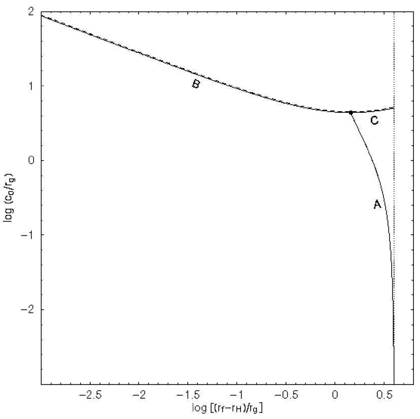
Figure 1: Solutions for $r_{\rm f}$—the radius at the fast critical point, corresponding to a magnetized flow with constant specific energy accreting onto a Schwarzschild black hole (solid curves). The parameter $c_{0}$, defined by Eq. (31), is proportional to the flux of radial magnetic field. The outer boundary of the flow is at the marginally stable circular orbit: $r_{0}=r_{\rm ms}=6\,r_{\rm g}$ (dotted line), where $r_{\rm g}\equiv M$ is the gravitational radius. The specific energy of fluid particles is equal to that of a test particle moving on the marginally stable circular orbit. The solutions for $r_{\rm f}$ consist of three branches: A, B, and C, with intersection at the dark point. The dashed curve represents the boundary for physical solutions: beyond the dashed curve physical solutions do not exist (see the text). (The dashed curve is indeed coincident with the solid curves B and C. To make it visible, we have shifted the dashed curve upward a little bit.)

In Fig. 1 we show the solutions for $r_{\rm f}$ corresponding to $r_{0}=r_{\rm ms}$ , where $r_{\rm ms}=6\,r_{\rm g}$ is the radius at the marginally stable circular orbit bar72 , $r_{\rm g}\equiv M$ is the gravitational radius of the black hole. This represents the solutions in the plunging region from the inner boundary of a thin Keplerian disk to the horizon of the black hole. The solutions for $r_{\rm f}$, represented by the solid curves in the figure, consist of three branches: A, B, and C, intersecting at the dark point. The dashed curve represents the boundary for physical solutions to exist: above the dashed curve Eq. (75) is violated so physical solutions do not exist. (The dashed curve is indeed coincident with the solid curves B and C. To make it visible, in the figure we have shifted the dashed curve upward a little bit.) From Fig. 1 we see that, below the dark point (where $r=3.4477\,r_{\rm g}$, $c_{0}=4.4030\,r_{\rm g}$), $r_{\rm f}$ is uniquely determined by the value of $c_{0}$. As $c_{0}^{2}/r_{\rm g}^{2}\rightarrow 0\,$, $r_{\rm f}$ approaches the radius at the marginally stable circular orbit $r_{\rm ms}$ (the vertical dotted line). This is just what we expect for a weakly magnetized thin Keplerian disk: the (magneto)sonic point should not be far from the marginally stable circular orbit (muc82 ; abr89 ; afs02 and references therein). Above the dark point, multiple solutions for $r_{\rm f}$ exist. In this paper we focus on the situation of weak magnetic fields with $c_{0}^{2}/r_{\rm g}^{2}\ll 1$, so we do not discuss the solutions above the dark point in detail.

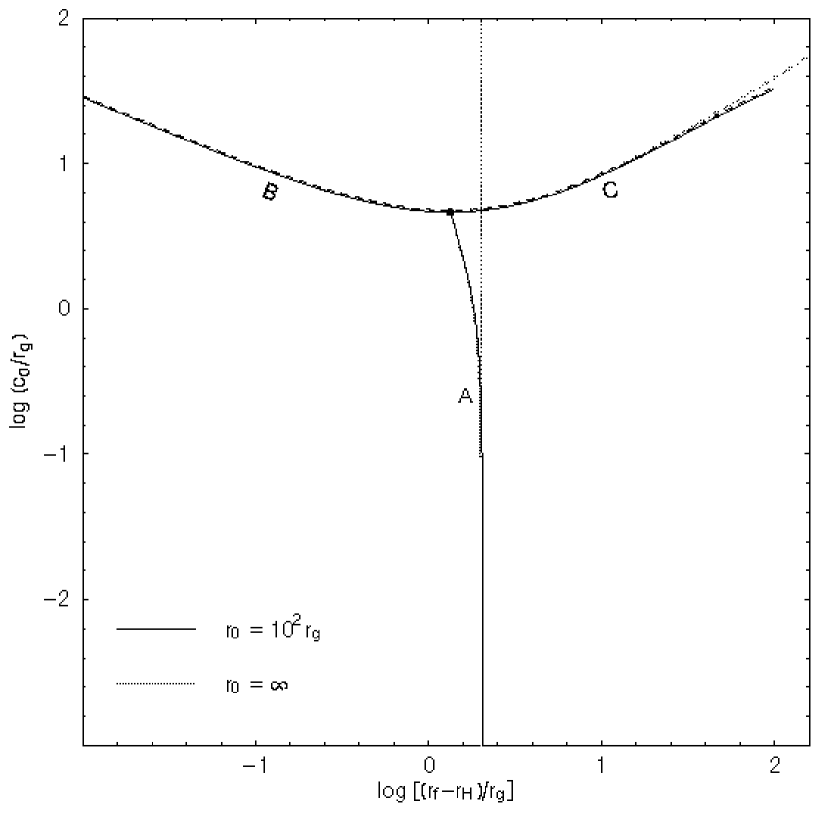
Figure 2: Same as Fig. 1 but for $r_{0}=10^{2}r_{\rm g}$ (dark lines) and $r_{0}=\infty$ (gray lines). The specific energy of fluid particles is equal to that of a test particle moving on a Keplerian circular orbit at $r=r_{0}$. The vertical dotted line marks the location of the marginally bound circular orbit ($r_{\rm mb}=4\,r_{\rm g}$).

We are more interested in solutions with $r_{0}\gg r_{\rm g}$, corresponding to a magnetized flow accreting onto a black hole from large radii. In Fig. 2 we show the solutions for $r_{\rm f}$ corresponding to $r_{0}=10^{2}r_{\rm g}$ (dark lines) and $r_{0}=\infty$ (gray lines). The solutions for $r_{0}\gg r_{\rm g}$ have the same topology as that for $r_{0}=r_{\rm ms}$. However, when $c_{0}/r_{\rm g}$ is fixed, $r_{\rm f}$ decreases as $r_{0}$ increases. For $r_{0}\gg r_{\rm g}$, $r_{\rm f}$ becomes insensitive to the value of $r_{0}$: on branches A and B the solutions for $r_{0}=10^{2}r_{\rm g}$ are almost indistinguishable from those for $r_{0}=\infty$. This is caused by the fact that $f_{\rm E}\approx-1$ for $r_{0}\gg r_{\rm g}$. From Fig. 2 we see that, for the case of $r_{0}\gg r_{\rm g}$, $r_{\rm f}$ approaches the radius at the marginally bound circular orbit $r_{\rm mb}=4\,r_{\rm g}$ bar72 (the vertical dotted line) in the limit $c_{0}^{2}/r_{\rm g}^{2}\rightarrow 0\,$.

In both Figs. 1 and 2 the dashed curve is coincident with the solution branches B and C. So, the solution branches B and C correspond to $f_{\rm L}=0$ [see Eqs. (72) and (74)]. By Eq. (57), such solutions correspond to $L_{\rm H}=0$ since $\Omega_{\Psi}=\Omega_{\rm H}=0$. Thus, for a sufficiently strong magnetic field (corresponding to the branches B and C), fluid particles lose all of their angular momentum as they reach the horizon of the black hole.

Once $r_{\rm f}$, $u_{\rm f}^{r}$, and $f_{\rm L}$ are determined as functions of $c_{0}$ and $f_{\rm E}$, we can solve the radial momentum equation for the radial velocity $u^{r}$ as a function of radius $r$. However, generally it is not a simple thing to solve the algebraic equation $F(r,u^{r})=0$, which has singularities and multiple roots. In practice we would rather solve the first-order differential equation

$$\frac{d\ln u^{r}}{d\ln r}=-\frac{1-\frac{c_{0}^{2}}{r^{2}u^{r}}\left(1-\frac{4M}{r}\right)+\left[\left(u^{r}\right)^{2}-f_{\rm E}^{2}\right]\left(1-\frac{2M}{r}\right)^{-2}\left(1-\frac{3M}{r}\right)\left[1-\frac{c_{0}^{2}}{r^{2}u^{r}}\left(1-\frac{2M}{r}\right)\right]}{\left(u^{r}\right)^{2}\left(1-\frac{2M}{r}\right)^{-1}-\frac{c_{0}^{2}}{r^{2}u^{r}}\left(1-\frac{2M}{r}-f_{\rm E}^{2}\right)}\;,$$

(77)

which is obtained by substituting Eqs. (67) and (73) into Eq. (50). Note that the only singularity in Eq. (77) is the fast critical point.

We choose on each side of the fast critical point a pair of $(r_{i},u_{i}^{r})$, which can be obtained by solving the algebraic equation $F(r,u^{r})=0$ where initial guessed values can be obtained by visually checking the contour plot of $F$ versus $r$ and $u^{r}$. Then, starting from the point $(r_{i},u_{i}^{r})$, we integrate Eq. (77) inward and outward, toward the horizon of the black hole and the fast critical point if $(r_{i},u_{i}^{r})$ is on the left-hand side of the fast critical point, or toward the fast critical point and large radii if $(r_{i},u_{i}^{r})$ is on the right-hand side of the fast critical point. [The starting point $(r_{i},u_{i}^{r})$cannot be exactly at the fast critical point since the latter is a fixed point of the differential equation.]

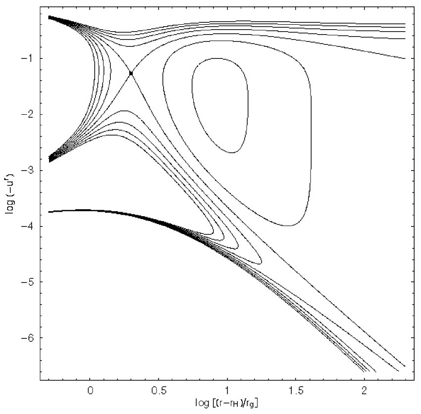
Figure 3: Contour plots of the generation function (66) versus $r$ and $u^{r}$. The parameters are: $c_{0}=0.1\,r_{\rm g}$, $f_{\rm E}=-1$, $f_{\rm L}=-3.96522\,r_{\rm g}$ (corresponding to $r_{0}=\infty$). Then, the fast critical point, which corresponds to a saddle point of the generation function, is at $(r_{\rm f},u_{\rm f}^{r})=(3.98852\,r_{\rm g},-0.053964)$, as indicated by the dark point. Contours are plotted from $F=-0.2$ to $F=0.2$ with step $\delta F=0.05$. The contours of $F=0$ are given by the two lines that smoothly pass the fast critical point, the one that goes from the right-bottom corner to the left-top corner represents the physical solution for the accretion flow.

As an example, we have solved the equation with $f_{\rm E}=-1$ (i.e., $r_{0}=\infty$) and $c_{0}=0.1\,r_{\rm g}$, corresponding to $r_{\rm f}=3.98852\,r_{\rm g}$ , $u_{\rm f}^{r}=-0.053964$ , and $f_{\rm L}=-3.96522\,r_{\rm g}$ . The contours of the corresponding generation function are plotted in Fig. 3 , from $F=-0.2$ to $F=0.2$ with step $\delta F=0.05$. The contours of $F=0$, which correspond to the physical solutions, are the two diagonal lines that smoothly pass the fast critical point at the dark point. The solution that we are interested in here should have $0<-u^{r}\ll 1$ at large radii and $u^{r}\sim-1$ near $r=r_{\rm H}$, which corresponds to the diagonal line that goes from the right-bottom corner to the left-top corner in Fig. 3. The differential radial momentum equation (77) is then solved along this diagonal line, with the approach described above.

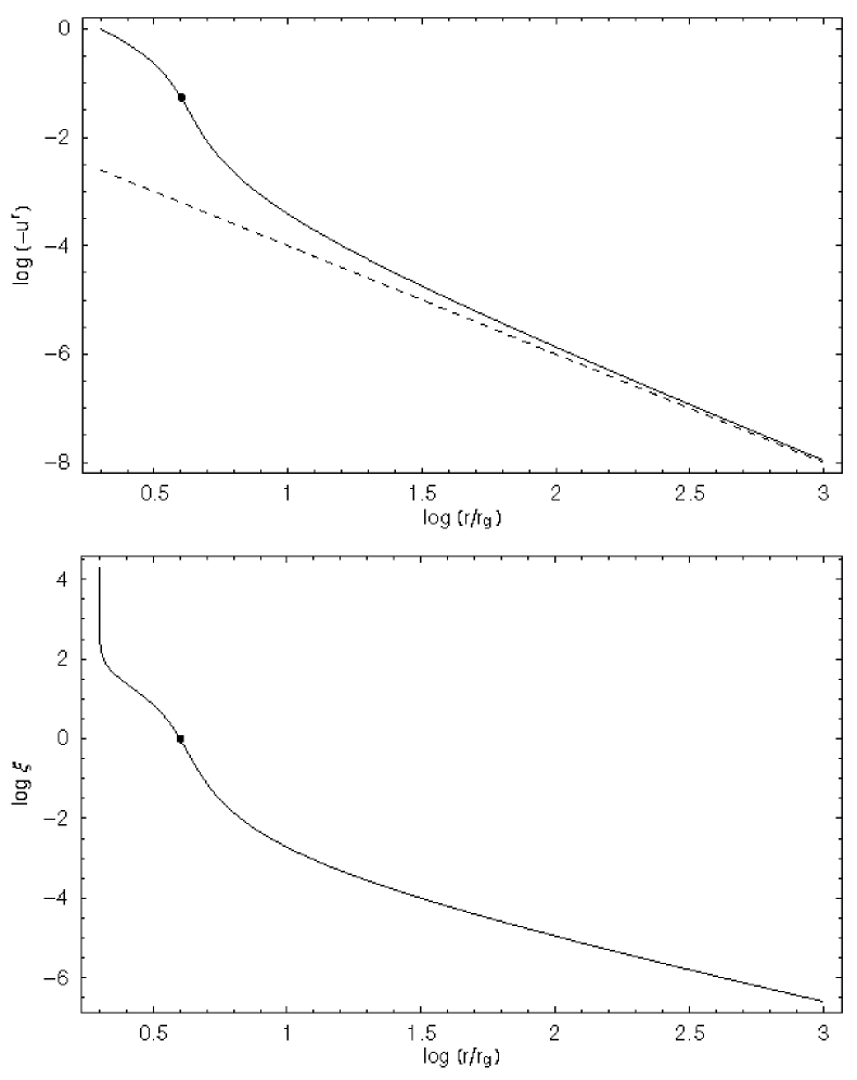
Figure 4: Upper panel: Solution to the radial momentum equation (77). The parameters are: $c_{0}=0.1\,r_{\rm g}$, $f_{\rm E}=-1$, and $f_{\rm L}=-3.96522\,r_{\rm g}$ (corresponding to $r_{0}=\infty$). The dark point shows the location of the fast critical point. The dashed line shows the asymptotic solution $u^{r}=-c_{0}^{2}/r^{2}$. Lower panel: The ratio $\xi=\left[u_{r}u^{r}\left(1-c_{\rm A}^{2}\right)/c_{\rm A}^{2}\right]^{1/2}$ corresponding to the solution in the upper panel. Subsonic motion corresponds to $\xi<1$. Supersonic motion corresponds to $\xi>1$. The fast critical point is at $\xi=1$, as indicated by the dark point.

The solution for the radial velocity $u^{r}$ as a function of $r$ is plotted in Fig. 4 (upper panel). For comparison, we show the asymptotic solution as $r\rightarrow\infty$ with the dashed line [see Eq. (62)]. We have calculated $\xi\equiv\left[u_{r}u^{r}\left(1-c_{\rm A}^{2}\right)/c_{\rm A}^{2}\right]^{1/2}$, and shown the results in the lower panel of Fig. 4. The parameter $\xi$ measures the ratio of the radial velocity to the Alfvén velocity. At the fast critical point we have $\xi=1$ [Eq. (54)]. The figure clearly shows that the flow starts from a subsonic state ($\xi<1$) at large $r$, passes the fast critical point at $r=r_{\rm f}$ ($\xi=1$), then enters a supersonic state ($\xi>1$) at $r<r_{\rm f}$. The ratio $\xi$ blows up at $r=r_{\rm H}$, confirming our analytic analysis in Sec. IV.2 [see Eq. (58)].

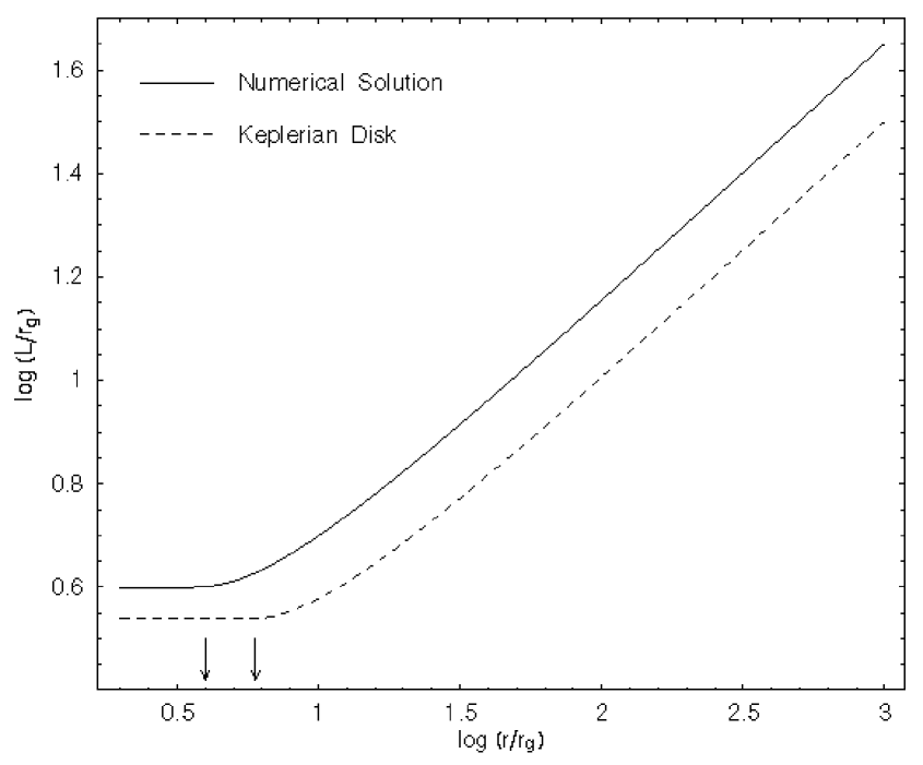
Figure 5: Evolution of the specific angular momentum of the particles in the flow described by the solution in Fig. 4 (solid line). The dashed line shows the solution corresponding to a thin Keplerian disk joined to a free-fall flow inside the marginally stable circular orbit. The two arrows show the locations of the fast critical point (left arrow) corresponding to the solution in Fig. 4, and the marginally stable circular orbit (right arrow).

The specific angular momentum of the fluid particles, $L$, can be calculated by substituting $a=\Psi=0$, and the solution $u^{r}(r)$ into Eq. (44). The results are shown in Fig. 5. For comparison, we show the specific angular momentum of a thin Keplerian disk with the dashed line. The Keplerian disk is joined to a free-fall flow in the plunging region, so its specific angular momentum keeps constant inside the marginally stable circular orbit. The fast critical point and the marginally stable circular orbit are indicated by two arrows (left and right, respectively). From Fig. 5 we see that, a disk flow with constant specific energy can lose angular momentum at a rate similar to that of a thin Keplerian disk.

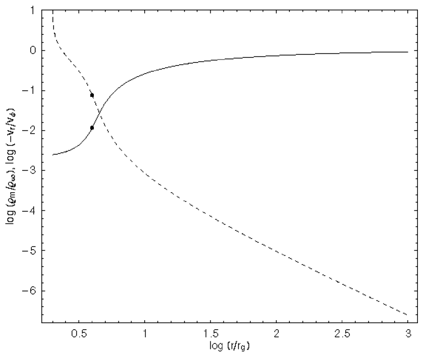
Figure 6: Evolution of the mass density (solid line) and the ratio of the radial velocity to the rotational velocity (dashed line), for the flow described by the solution in Fig. 4. The mass density is in units of its value at infinity: $\rho_{\infty}\equiv F_{\rm m}^{2}/\left(4\pi C_{0}^{2}\right)$ [see Eq. (64)]. The dark points show the location of the fast critical point.

Figure 5 shows that the specific angular momentum of the flow remains almost constant after the flow passes the fast critical point. This suggests that we can treat the fast critical point as an inner boundary of the accretion flow. To justify this, we have calculated the mass density of the flow and the ratio of the radial velocity to the rotational velocity, as functions of radius $r$. The mass density of the flow is simply given by Eq. (27), which approaches a constant as $r\rightarrow\infty$ [Eq. (64)]. The ratio of the radial velocity to the rotational velocity, as measured by a local static observer, is given by $v_{r}/v_{\phi}=ru^{r}/\chi L$ . The numerical results for the mass density and the ratio of the radial velocity to the rotational velocity, corresponding to the solution in Fig. 4, are shown in Fig. 6.

We see that, at large radii $|v_{r}/v_{\phi}|\ll 1$, and $\rho_{\rm m}\rightarrow\rho_{\infty}\equiv F_{\rm m}^{2}/\left(4\pi C_{0}^{2}\right)$ [Eq. (64)]. As the flow gets close to and passes the fast critical point (the dark points in the figure), $\rho_{\rm m}/\rho_{\infty}$ drops quickly and $|v_{r}/v_{\phi}|$ increases quickly. At the fast critical point we have $\rho_{\rm m}=0.01167\,\rho_{\infty}$ and $v_{r}=-0.07629\,v_{\phi}$ . These numbers support the point that the fast critical point behaves like an inner boundary of the disk accretion flow: it marks the transition of the flow from a state with $|v_{r}/v_{\phi}|\ll 1$ at large radii to a state with $|v_{r}/v_{\phi}|\gtrsim 1$ near the horizon of the black hole. Beyond the inner boundary, the magnetic field plays an important role in the dynamics of the flow and transports angular momentum outward. Inside the inner boundary, the dynamical effects of the magnetic field become unimportant and the fluid particles free-fall to the horizon of the black hole (Fig. 5).

Figure 6 also shows that, as $r\rightarrow r_{\rm H}$, $\rho_{\rm m}$ is finite but $|v_{r}/v_{\phi}|$ blows up. The former is because of the fact that $u^{r}$ is finite at $r=r_{\rm H}$ (see Sec. IV.2), the latter is caused by the well-known fact that $v_{\phi}\rightarrow 0$ and $v_{r}\rightarrow-1$ as particles approach the horizon.

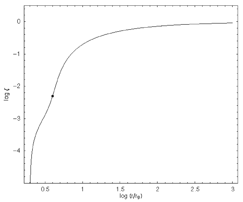
Figure 7: The ratio of the magnetic energy density to the kinetic energy density [defined by Eq. (59)] corresponding to the solution in Fig. 4. The dark point shows the location of the fast critical point.

The ratio of the magnetic energy density to the kinetic energy density of the flow, as measured by a local static observer [see Eq. (59); note that when $a=\Psi=0$ the electric field is zero, see Eq. (15)], is calculated and shown in Fig. 7. In the region of $r\gg r_{\rm f}$, the ratio $\zeta$ is $\approx 1$, i.e., the energy of the magnetic field is about equipartitioned with the kinetic energy of the flow [Eq. (65)]. This is caused by the fact that for $r\gg r_{\rm f}$ the velocity of the flow is predominantly rotational: $|v_{r}/v_{\phi}|\ll 1$ (Fig. 6), so the magnetic field is sufficiently amplified by the shear rotation until the energy density of the magnetic field is comparable to the kinetic energy density of the flow. In the region of $r\lesssim r_{\rm f}$, we have $\zeta\ll 1$, caused by the fact that for $r\lesssim r_{\rm f}$ the radial component of the flow velocity becomes comparable to, or even greater than the azimuthal component (Fig. 6), then the amplification of the magnetic field by the shear motion becomes unimportant li03 . At the fast critical point (the dark point in the figure), we have $\zeta=0.004954\,$. As $r\rightarrow r_{\rm H}$, we have $\zeta\rightarrow 0\,$.

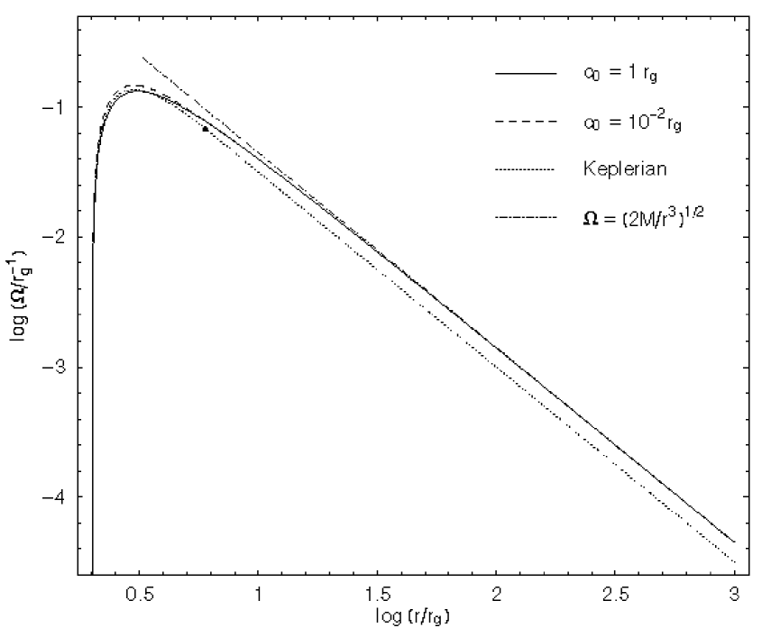
Figure 8: The angular velocity of a flow with $f_{\rm E}=-1$. The parameter $c_{0}$ is alternatively assumed to be $1\,r_{\rm g}$ (solid line) and $10^{-2}\,r_{\rm g}$ (dashed line). The dotted line shows the angular velocity of a thin Keplerian disk joined to a free-fall flow inside the marginally stable circular orbit (the dark point). The dashed-dotted line represents the asymptotic solution given by Eq. (63).

To see how sensitive the solutions are to the variation of $c_{0}$, and how the solutions approach the asymptotic solutions at infinity found in Sec. IV.3, we have solved the radial momentum equation with $f_{\rm E}=-1$ corresponding to two different values of $c_{0}$: $c_{0}=1\,r_{\rm g}$ and $c_{0}=10^{-2}r_{\rm g}$. The solutions for the angular velocity $\Omega=u^{\phi}/u^{t}$ are shown in Fig. 8. The solid line corresponds to $c_{0}=1\,r_{\rm g}$, the dashed line to $c_{0}=10^{-2}r_{\rm g}$. The dotted line in the figure is the angular velocity of a thin Keplerian disk joined to a free-fall flow in the plunging region. The dashed-dotted line shows the asymptotic solution for $\Omega$ derived from Eq. (63). We see that, the solutions are insensitive to the value of $c_{0}$ for $c_{0}^{2}\lesssim r_{\rm g}^{2}$, and they are well represented by the asymptotic solution in the region with $\log(r/r_{\rm g})>1.5\,$.

V.2 Solutions around a Kerr black hole

The spin of the black hole has important effects on the solutions of an accretion flow near the horizon of the black hole. For example, for the case of a thin Keplerian disk, the spin of the black hole determines the location of the inner boundary of the disk, how much energy is dissipated in the disk, and how much angular momentum is carried into the black hole by the flow nov73 ; Page & Thorne (1974); tho74 . In this subsection we show how the spin of the black hole affects the accretion process by presenting some solutions for a magnetized flow with constant specific energy accreting onto a Kerr black hole. We assume that at large radii the specific angular momentum of the disk is always positive, but the specific spinning angular momentum of the black hole, $a$, can be either positive or negative.

For the case of a Kerr black hole with $\Psi=0$, the generation function becomes

$$F(r,u^{r}) = \left[1+\frac{c_{0}^{2}}{r^{2}u^{r}}\left(1-\frac{2M}{r}\right)\right]^{2}\left[\frac{r^{2}}{\Delta}\left(u^{r}\right)^{2}+1-\frac{f_{\rm E}^{2}}{1-\frac{2M}{r}}\right]$$ (78)

$$+\;\frac{\left[\frac{2Ma}{r}f_{\rm E}+\left(1-\frac{2M}{r}\right)f_{\rm L}\right]^{2}}{\Delta\left(1-\frac{2M}{r}\right)}\;.$$

The derivative of $F$ with respect to $u^{r}$ is

$$\frac{\partial F}{\partial u^{r}}=\frac{2}{u^{r}}\left[1+\frac{c_{0}^{2}}{r^{2}u^{r}}\left(1-\frac{2M}{r}\right)\right]\left[\frac{r^{2}}{\Delta}\left(u^{r}\right)^{2}-\frac{c_{0}^{2}}{r^{2}u^{r}}\left(1-\frac{2M}{r}-f_{\rm E}^{2}\right)\right]\;.$$ (79)

The derivative of $F$ with respect to $r$ is too lengthy so we do not write it out here.

The radial velocity at the fast critical point can be solved from $\left.\partial F/\partial u^{r}\right|_{r=r_{\rm f}}=0$

$$u_{\rm f}^{r}=-\left[\frac{c_{0}^{2}\Delta_{\rm f}}{r_{\rm f}^{4}}\left(-1+\frac{2M}{r_{\rm f}}+f_{\rm E}^{2}\right)\right]^{1/3}\;,\hskip 28.45274pt\Delta_{\rm f}\equiv\Delta(r=r_{\rm f})\;.$$ (80)

From the radial momentum equation $F(r,u^{r})=0$, we can solve for $f_{\rm L}$

$$f_{\rm L} = -\frac{1}{1-\frac{2M}{r}}\left\{\frac{2Ma}{r}f_{\rm E}+\left[1+\frac{c_{0}^{2}}{r^{2}u^{r}}\left(1-\frac{2M}{r}\right)\right]\right.$$ (81)

$$\left.\times\left[-\left(1-\frac{2M}{r}\right)\left(ru^{r}\right)^{2}-\Delta\left(1-\frac{2M}{r}-f_{\rm E}^{2}\right)\right]^{1/2}\right\}\;.$$

Substituting Eq. (81) into the expression for $\partial F/\partial r$, we can eliminate $f_{\rm L}$ from $\partial F/\partial r$. Then, similar to the case of a Schwarzschild black hole, we can obtain $r_{\rm f}$ and $u_{\rm f}^{r}$ by solving the joined equations (80) and $\partial F/\partial r=0$. Then by Eq. (81) we can determine $f_{\rm L}=f_{\rm L}(c_{0},f_{\rm E})$.

For physical solutions $f_{\rm L}$ must be real, so the following condition must be satisfied

$$-\left(1-\frac{2M}{r}\right)\left(ru^{r}\right)^{2}-\Delta\left(1-\frac{2M}{r}-f_{\rm E}^{2}\right)\geq 0\;.$$ (82)

Making use of Eq. (80), at $r=r_{\rm f}$ Eq. (82) becomes

$$\left(1-\frac{2M}{r_{\rm f}}\right)^{3}\,\frac{c_{0}^{4}}{r_{\rm f}^{2}}\leq\Delta_{\rm f}\left(-1+\frac{2M}{r_{\rm f}}+f_{\rm E}^{2}\right)\;.$$ (83)

As in the case of a Schwarzschild black hole, Eq. (83) provides a constraint on the region in the $(r_{\rm f},c_{0})$ space where physical solutions exist, whence $f_{\rm E}$ is specified.

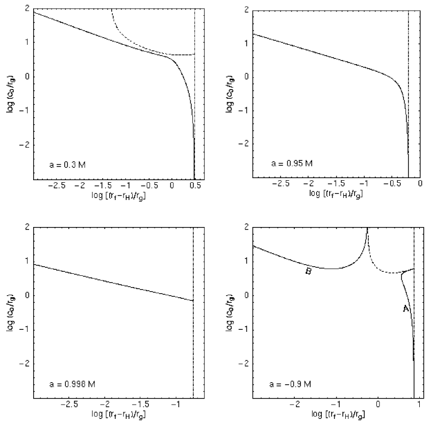
Figure 9: Solutions for $r_{\rm f}$—the radius at the fast critical point corresponding to a flow with constant specific energy accreting onto a Kerr black hole (solid curves). Each panel corresponds to a different spinning state of the black hole, as indicated by the value of $a$. The outer boundary of the flow is at the marginally stable circular orbit: $r_{0}=r_{\rm ms}(a)$, as indicated by the vertical dotted line. The specific energy of fluid particles is assumed to be equal to that of a test particle moving on a Keplerian circular orbit at $r_{0}=r_{\rm ms}(a)$. The dashed curve represents the boundary for physical solutions: beyond the dashed curve physical solutions do not exist (see the text).

In Fig. 9 we show the solutions for $r_{\rm f}$ with $r_{0}=r_{\rm ms}(a)$ and $f_{\rm E}=-E_{\rm Keplerian}(r_{0},a)$, where $E_{\rm Keplerian}(r_{0},a)$ is the specific energy of a test particle moving on a Keplerian circular orbit around a Kerr black hole at $r=r_{0}$ bar72 ; nov73 ; Page & Thorne (1974). Each panel corresponds to a different spinning state of the black hole. The dashed curve shows the boundary for physical solutions: above the dashed curve Eq. (83) is violated so physical solutions do not exist. For the cases of $a/M=0.95$ and $0.998$, we have $r_{\rm ms}<2M$ and Eq. (83) is always satisfied since the right-hand side is always positive [see Eq. (80) where $u_{\rm f}^{r}<0$]. So, the dashed curve does not appear in the panels corresponding to $a/M=0.95$ and $0.998$. In the case of $a/M=-0.9$, there are two branches of solutions for $r_{\rm f}$, labeled by A and B. This is a general feature for the case of $a<0$. Like in the case of a Schwarzschild black hole, in the limit of $c_{0}^{2}/r_{\rm g}^{2}\rightarrow 0$, $r_{\rm f}$ approaches $r_{\rm ms}$, except for the case of $a/M$ very close to $1$, e.g., $a/M=0.998$. In the case of $a/M=0.998$, solutions for $r_{\rm f}$ do not exist if $c_{0}^{2}/r_{\rm g}^{2}$ is sufficiently small. This means that for sufficiently small $c_{0}^{2}/r_{\rm g}^{2}$, the flow is already supersonic as it leaves the marginally stable circular orbit. This is caused by the fact that we have neglected the gas pressure in our treatment. In the Keplerian disk region ($r>r_{\rm ms}$) the gas pressure cannot always be neglected—especially near the inner boundary ($r\approx r_{\rm ms}$). When the gas pressure is included, it will make the radial motion subsonic in the disk region and give rise to a sonic point close to the marginally stable circular orbit (muc82 ; abr89 ; afs02 ).

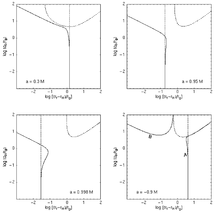
Figure 10: Same as Fig. 9 but $r_{0}=\infty$. The specific energy of fluid particles is assumed to be equal to $1$. The vertical dotted line marks the location of the marginally bound circular orbit, $r_{\rm mb}(a)$.

In Fig. 10 we show the solutions for $r_{\rm f}$ with $r_{0}=\infty$ and $f_{\rm E}=-1$. Similar to the case of a Schwarzschild black hole, when $c_{0}^{2}/r_{\rm g}^{2}\ll 1$ the fast critical point approaches the marginally bound circular orbit: $r_{\rm f}\approx r_{\rm mb}$, where $r_{\rm mb}=2M\left[1-a/2M+(1-a/M)^{1/2}\right]$ bar72 .

By comparing Figs. 9 and 10 with Figs. 1 and 2, we can see how the topology of the solutions for $r_{\rm f}$ evolves with the spin of the black hole. For $a<0$, the solutions have two branches: A and B. As $a/M$ increases from $-1$ to $0$, the branch B moves toward left. (One can check this by solving $r_{\rm f}$ for a negative $a>-0.9$.) As $a$ approaches $0^{-}$, the branch $B$ of negative $a$ disappears, the branch $A$ of negative $a$ becomes the branches A and C of $a=0$. For $a>0$, the solutions have only one branch. As $a/M$ decreases from $1$ to $0^{+}$, the branch of positive $a$ becomes the branches A and B of $a=0$.

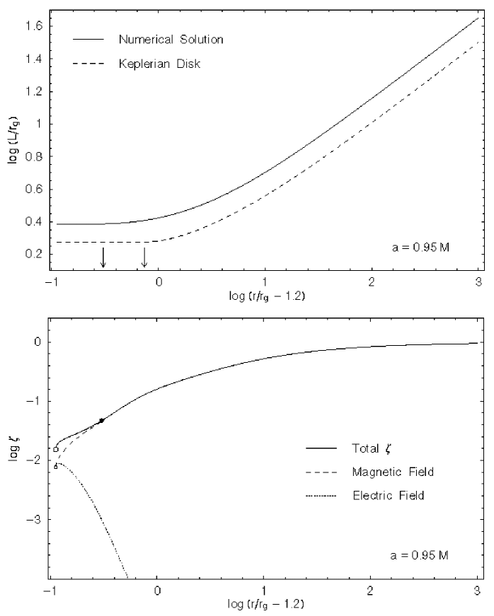
Figure 11: Upper panel: Evolution of the specific angular momentum of a flow with constant specific energy accreting onto a Kerr black hole with $a/M=0.95$. The dashed curve shows the solution corresponding to a thin Keplerian disk joined to a free-fall flow inside the marginally stable circular orbit. The two arrows show the locations of the fast critical point (left) and the marginally stable circular orbit (right). Lower panel: Ratio of the electromagnetic energy density to the kinetic energy density (solid line) corresponding to the solution in the upper panel, which consists of the contributions of magnetic field (dashed line) and electric field (dotted line). The dark point shows the location of the fast critical point. The circles show location of the horizon. (The unit of the horizontal axis is chosen to make the structure near the horizon clear.)

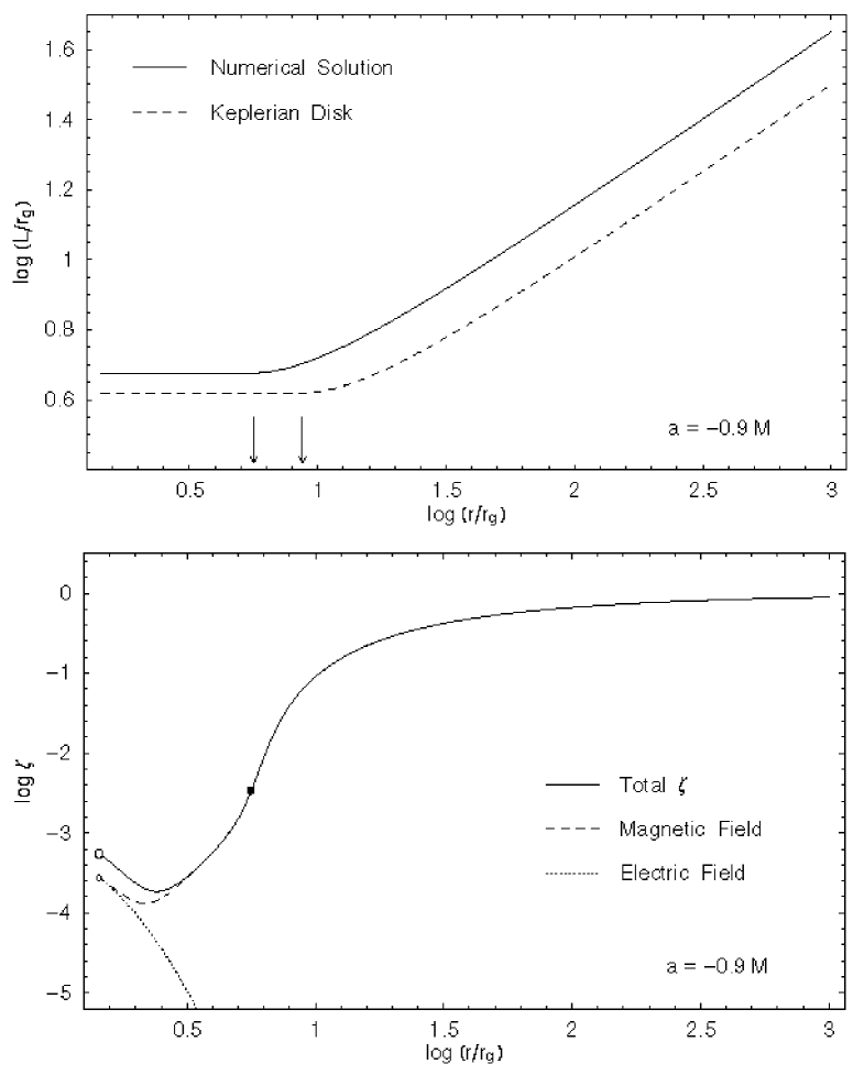
Figure 12: Same as Fig. 11 but for $a/M=-0.9$.

As examples, we have solved the radial momentum equation for a Kerr black hole with $a/M=0.95$ and $a/M=-0.9$, respectively. We assume that $c_{0}=0.1\,r_{\rm g}$ and $f_{\rm E}=-1$ (i.e., $r_{0}=\infty$). In Fig. 11 we show the specific angular momentum of fluid particles (upper panel), and the ratio of the electromagnetic energy density to the kinetic energy density as measured by a LNRF observer [lower panel, defined by Eq. (59)] for the case of $a/M=0.95$. In the upper panel, the dashed curve shows the corresponding solution for a thin Keplerian disk joined to a free-fall flow inside the marginally stable circular orbit. The two arrows show the positions of the fast critical point (left) and the marginally stable circular orbit (right). In the lower panel, in addition to the total $\zeta$ (solid line), we also show the contribution from the magnetic field (dashed line) and the electric field (dotted line) separately. The dark point on the solid line shows the location of the fast critical point. The two circles show the location of the black hole horizon. Solutions for the specific angular momentum and the ratio of the electromagnetic energy density to the kinetic energy density for the case of $a/M=-0.9$ are shown in Fig. 12.

From Figs. 11 and 12 we see that, similar to the case of a Schwarzschild black hole, the specific angular momentum of the fluid particles is effectively removed by the magnetic field, though the specific energy keeps constant during the motion. However, the specific angular momentum of the fluid particles as they reach the horizon of the black hole depends on the spin of the black hole, which can be seen by comparing Figs. 11 and 12 with Fig. 5.

At large radii the energy of the electromagnetic field is about equipartitioned with the kinetic energy of the particles, while near and inside the fast critical point the ratio of the electromagnetic energy density to the kinetic energy density drops to values $\ll 1$. However, unlike the case for a Schwarzschild black hole, the ratio is not zero on the horizon of the black hole when $a\neq 0$. This is related to the fact that when $a\neq 0$ the magnetic field is not aligned with the velocity field near the horizon (caused by the frame dragging effect, see Sec. II), resulting a nonzero electric field as shown by the dotted lines in the two figures (lower panels). On the horizon the ratio of the electric energy density to the magnetic energy density approaches $1$, so the dashed line and the dotted line end on the same small circle. The strength of the electric field drops quickly as the radius increases, and at large radii (where $E_{a}^{\prime}E^{\prime a}\propto r^{-8}$, $B_{a}^{\prime}B^{\prime a}\propto r^{-1}$) the effect of the electric field is negligible.

The fact that the ratio of the electromagnetic energy density to the kinetic energy density is small near and inside the fast critical point, for both the Schwarzschild case and the Kerr case, explains why the fast critical point approaches the marginally bound circular orbit in the limit of $r_{0}\gg r_{\rm g}$ and $c_{0}^{2}/r_{\rm g}^{2}\ll 1$, because then $E\approx 1$ and the dynamical effects of the electromagnetic field are unimportant near and inside the fast critical point. The results support the point that the fast critical point behaves like an inner boundary of the flow, beyond which the dynamical effects of the magnetic field are important, inside which the dynamical effects of the magnetic field are negligible and fluid particles free-fall to the black hole.

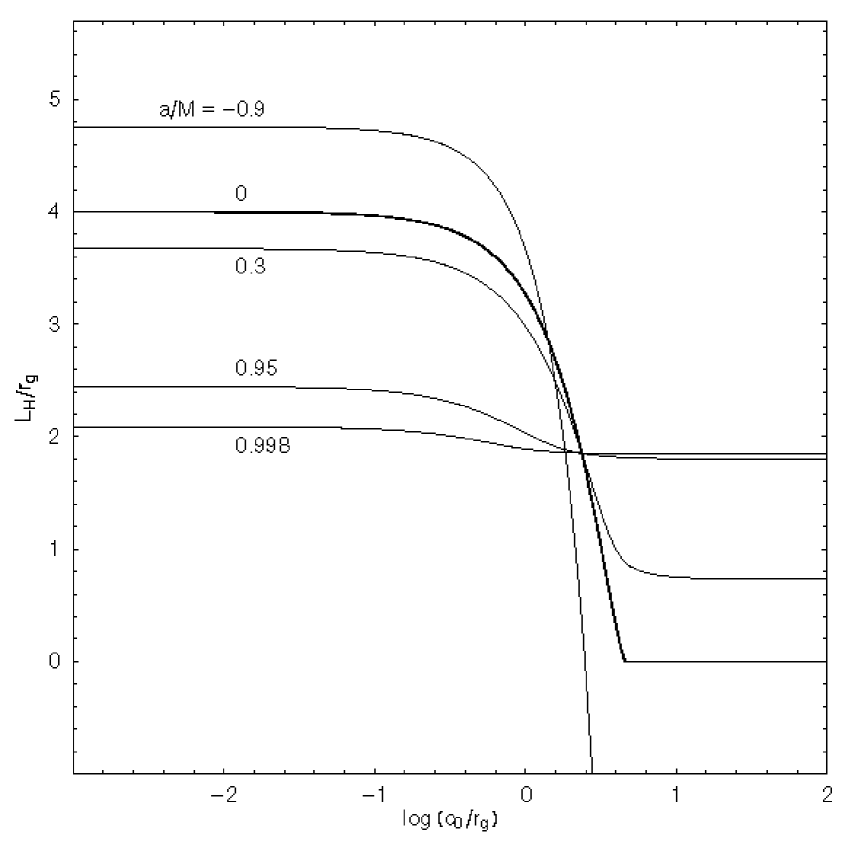
Figure 13: The specific angular momentum of fluid particles as they reach the horizon of the black hole, as a function of $c_{0}$. Different curves correspond to different spinning states of the black hole as labeled. The outer boundary of the flow is at $r_{0}=\infty$ so $f_{\rm E}=-1$. (At large radii the specific angular momentum is $\propto r^{1/2}$, so $L=\infty$ at $r_{0}=\infty$.)

In Sec. IV.2 we have shown that the specific angular momentum of the fluid particles on the horizon of the black hole is given by Eq. (57). For solutions that smoothly pass the fast critical point, the parameter $f_{\rm L}$ is determined as a function of $f_{\rm E}$ and $c_{0}$ when $\Psi=0$. Hence, if $f_{\rm E}$ is specified, for a given spin of the black hole $L_{\rm H}$ depends only on $c_{0}$. In Fig. 13, we show $L_{\rm H}$ as a function of $c_{0}$, where different curves correspond to different spinning states of the black hole. The outer boundary of the flow is assumed to be at infinity so that $f_{\rm E}=-1$. Figure 13 confirms the results in Figs. 5, 11, and 12. Furthermore, we see that $L_{\rm H}$ depends on $a$ in opposite ways for small and large $c_{0}$: for small $c_{0}$, $L_{\rm H}$ decreases with increasing $a$; for large $c_{0}$, $L_{\rm H}$ increases with increasing $a$. And, for sufficiently large $c_{0}$, $L_{\rm H}$ becomes zero when $a=0$ (see Sec. V.1). For large $c_{0}$ and negative $a$, $L_{\rm H}$ is negative. The $L_{\rm H}$ corresponding to positive $a$ is always positive.

VI Discussion: The Effect of Finite Resistivity and Different Evolution of Large and Small-Scale Magnetic Fields

The solutions that we have found have the following unique feature: the magnetic field is aligned with the velocity field [Eq. (16)]; and, as a result, at large radii the energy of the magnetic field is equipartitioned with the kinetic energy of the flow [Eq. (65)]. The latter is obvious from the following consideration: At large radii, where the gravity is approximately Newtonian and the radial flux of angular momentum is not important, we have $4\pi\rho_{\rm m}u^{r}u^{\phi}\approx B^{r}B^{\phi}$. Then, $B^{r}/B^{\phi}=u^{r}/u^{\phi}$ implies that $B_{r}B^{r}\approx 4\pi\rho_{\rm m}u_{r}u^{r}$ and $B_{\phi}B^{\phi}\approx 4\pi\rho_{\rm m}u_{\phi}u^{\phi}$, i.e., $B^{2}/8\pi\approx\rho_{\rm m}v^{2}/2$, where $B^{2}=B_{r}B^{r}+B_{\phi}B^{\phi}$ and $v^{2}=u_{r}u^{r}+u_{\phi}u^{\phi}$. An almost inverse statement is also true: If at large radii $B_{\phi}B^{\phi}\approx 4\pi\rho_{\rm m}u_{\phi}u^{\phi}$, then we must have $B^{r}/B^{\phi}\approx u^{r}/u^{\phi}$ at large radii. (See App. B for the corresponding solutions for a Newtonian accretion disk.)

The above results rely on the fact that we have neglected all energy dissipation processes by assuming a perfectly conducting fluid with zero resistivity and viscosity. In the Newtonian limit (which is valid at large distances from the central black hole), the induction equation including a finite electric resistivity $\eta$ is given by (see, e.g., bal98 )

$$\frac{\partial{\bf B}}{\partial t}=\nabla\times\left({\bf v}\times{\bf B}-\frac{\eta}{4\pi}\nabla\times{\bf B}\right)\;.$$ (84)

We assume that $\eta=\mbox{constant}$. Then, substitute Eq. (114) into Eq. (84), we obtain the stationary and axisymmetric solution

$$r\left(v_{r}B_{\phi}-v_{\phi}B_{r}\right)=\frac{\eta}{4\pi}\frac{d}{dr}\left(rB_{\phi}\right)+C\;,$$ (85)

where $C$ is an integral constant.

To estimate the effect of finite resistivity, let us consider the case of $C=0$. Then from Eq. (85) we have

$$\frac{B_{r}}{B_{\phi}}=\zeta_{\rm M}\,\frac{v_{r}}{v_{\phi}}\;,\hskip 28.45274pt\zeta_{\rm M}\equiv 1-\frac{\eta}{4\pi rv_{r}}\frac{d\ln\left(rB_{\phi}\right)}{d\ln r}\;.$$ (86)

The parameter $\zeta_{\rm M}$ determines the orientation of the magnetic field relative to the velocity field in the $r-\phi$ plane. Define

$$R_{\rm M}\equiv\frac{8\pi^{2}r\left|v_{\phi}\right|}{\eta}\;,\hskip 28.45274ptq\equiv\frac{d\ln\left(rB_{\phi}\right)}{d\ln r}\;,$$ (87)

where $R_{\rm M}$ is the magnetic Reynolds number associated with the azimuthal motion, $q$ measures the radial gradient of the magnetic field. Then, $\zeta_{\rm M}$ can then be rewritten as

$$\zeta_{\rm M}=1+\frac{1}{\lambda}\;,\hskip 28.45274pt\lambda\equiv\frac{R_{\rm M}}{2\pi q}\left|\frac{v_{r}}{v_{\phi}}\right|\;.$$ (88)

Therefore, the effect of finite resistivity is determined by the parameter $\lambda$. When $|\lambda|\gg 1$, we have $\zeta_{\rm M}\approx 1$, the effect of resistivity is unimportant and the solutions correspond to a perfectly conducting fluid as in the case of our analytical model. Then, the magnetic field is aligned with the velocity field and the magnetic energy density is equipartitioned with the rotational energy density of the disk at large radii. When $|\lambda|\ll 1$, we have $|\zeta_{\rm M}|\approx 1/|\lambda|\gg 1$, the effect of resistivity becomes important and the solutions correspond to a nonperfectly conducting fluid. The magnetic field is not aligned with the velocity field, resulting significant energy transportation and dissipation. Then, in the stationary state the magnetic energy density should be much smaller than the rotational energy density of the disk (as shown bellow). The effect of finite resistivity is particular important for small-scale and chaotic magnetic fields that reverse directions frequently, since at places where $B_{\phi}=0$ but $dB_{\phi}/dr\neq 0$ we have $|q|=\infty$ [Eq. (87)] and $\lambda=0$.

It is the assumption of a perfectly conducting fluid with zero resistivity and viscosity that makes our analytical results different from the MHD numerical simulation results, where the magnetic field is not always aligned with the velocity field and the energy density of the magnetic field is usually much smaller than the rotational energy density of disk particles (see, e.g., sto96 ; haw96 ; haw00 ; haw01 ; haw02 ; ste02 ). In numerical simulations, finite resistivity and energy dissipation arising from finite spatial gridding in numerical codes always exist and are often large, even though the physical resistivity and viscosity can be assumed to be zero haw95 ; ryu95 . In fact, in current three-dimensional MHD simulations, the Reynolds number arising from finite numerical gridding is often smaller than the magnetic Reynolds number associated with most astrophysical plasmas haw95 ; haw01a .

How about the effect of finite resistivity in real astronomy? For astrophysical plasmas, the magnetic Reynolds number $R_{\rm M}$ is usually extremely large ($\gtrsim 10^{6}$) due to small microscopic Ohmic resistivity and large spatial scales and velocities (see, e.g., cho98 ). However, dissipation processes like convection, turbulence, etc, can induce a large effective resistivity kra80 ; pud81a ; pud81b ; mes99 , thus produce a smaller magnetic Reynolds number. The parameter $q$ can also be large if the magnetic field has small scales and is chaotic.

For an ordered large-scale magnetic field we usually have $q\sim 1$ in regions where $B_{\phi}\neq 0$. While for small-scale and chaotic magnetic fields, the parameter $q$ can be very large, especially at places where $B_{\phi}=0$. In this latter case, the accretion disk cannot always be described with a simple stationary and axisymmetric model without using a statistical approach. We can define a coherent length scale $l_{\rm c}$ so that $|q|\sim r/l_{\rm c}$. Then, $\lambda$ in Eq. (88) can be recast as

$$\lambda\sim\frac{R_{\rm c}}{2\pi}\left|\frac{v_{r}}{v_{\rm c}}\right|\;,\hskip 28.45274ptR_{\rm c}\equiv\frac{8\pi^{2}l_{\rm c}v_{\rm c}}{\eta}\;,$$ (89)

where $v_{\rm c}$ is the velocity associated with the local coherent structure, $R_{\rm c}$ is the corresponding magnetic Reynolds number, and $\eta$ is the resistivity in the disk.

Thus, accretion disks driven by large-scale magnetic fields behave very differently from those driven by small-scale magnetic fields. For an accretion disk driven by a large-scale magnetic field, like the model studied in this paper, $\lambda$ is usually $\gg 1$ (since $q\sim 1$) and determined by the global motion of the disk through $R_{\rm M}$ and $v_{r}/v_{\phi}$ [Eq. (88)]. For an accretion disk driven by small-scale magnetic fields, $\lambda$ is usually $\ll 1$ (since $|q|\gg 1$) and determined by $R_{\rm c}$ and $v_{r}/v_{c}$ [Eq. (89)]. In this latter case, the global motion affects $\lambda$ (so affects the equilibrium state) only through the radial velocity $v_{r}$—the global rotation of the disk has no effect on $\lambda$ (so does not affect the equilibrium state of the magnetic field).

Making use of Eq. (86) and $4\pi\rho_{\rm m}v_{r}v_{\phi}\approx B_{r}B_{\phi}$, we can estimate the energy density of the magnetic field by

$$\frac{{\cal E}_{\rm M}}{{\cal E}_{\rm K}}\approx\frac{\zeta_{\rm M}^{-1}+\zeta_{\rm M}\left(v_{r}/v_{\phi}\right)^{2}}{1+\left(v_{r}/v_{\phi}\right)^{2}}\;,$$ (90)

where ${\cal E}_{\rm M}=(1/8\pi)\left(B_{r}^{2}+B_{\phi}^{2}\right)$ is the magnetic energy density, ${\cal E}_{\rm K}=\left(\rho_{\rm m}/2\right)\left(v_{r}^{2}+v_{\phi}^{2}\right)$ is the kinetic energy density of the disk. When $\lambda\gg 1$ (corresponding to large-scale magnetic fields), we have ${\cal E}_{\rm M}\approx{\cal E}_{\rm K}$, the magnetic energy is approximately equipartitioned with the rotational energy of the disk (recall that $\left|v_{r}/v_{\phi}\right|\ll 1$). When $\lambda\ll 1$ (corresponding to small-scale magnetic fields), we have ${\cal E}_{\rm M}/{\cal E}_{\rm K}\sim\left(R_{\rm c}/2\pi\right)\left|v_{r}/v_{\phi}\right|\sim\lambda\left|v_{\rm c}/v_{\phi}\right|\ll 1$, the magnetic energy density is much smaller than the rotational energy density of the disk. As an example for an accretion disk with small-scale magnetic fields, consider a thin Keplerian disk with $\left|v_{r}\right|\sim v_{\rm c}^{2}/\left|v_{\phi}\right|$ where $v_{\rm c}$ corresponds to the fluctuation in the fluid velocity arising from turbulence bal98 , and $R_{\rm c}\sim 2\pi$ (see, e.g., mes99 ), then we have ${\cal E}_{\rm M}\sim\rho_{\rm m}v_{\rm c}^{2}/2$, i.e., the magnetic energy density is approximately equipartitioned with the kinetic energy density in turbulence. Thus, for a disk with small-scale magnetic fields the equilibrium state is determined by the local turbulent motion rather than the global rotation pud81a ; pud81b .

Based on the above arguments, we believe that the results of Gammie gam99 are more relevant to a large-scale magnetic field connecting the disk to the black hole, rather than small-scale and chaotic magnetic fields in the plunging region.

VII Summary and Conclusions

With an analytical model we have investigated the dynamics of a cold accretion disk containing a large-scale magnetic field around a Kerr black hole, trying to understand the process of angular momentum and energy transportation. A one-dimensional radial momentum equation is derived near the equatorial plane of the black hole, which has one intrinsic singularity at the fast critical point. Any physical solution corresponding to an accretion flow starting from infinity subsonically must smoothly pass the fast critical point in order to reach the horizon of the black hole. Because of this requirement, among the four integral constants ($c_{0}$, $\Omega_{\Psi}$, $f_{\rm L}$, and $f_{\rm E}$) only three are independent: one of them has to be determined as a function of the other three.

In order for $r^{2}B^{r}$ and $B^{2}/4\pi\rho_{\rm m}$ to be finite at infinity, the constant $\Omega_{\Psi}$ has to be zero (Secs. II and III.1). This indicates that in the stationary state the magnetic field and the velocity field of the fluid must be parallel to each other. When this condition is satisfied ($\Omega_{\Psi}=0$), the specific energy of the fluid particles remains constant during the motion, but the specific angular momentum changes.

The radial momentum equation has been solved with the assumptions that $\Omega_{\Psi}=0$, $c_{0}^{2}/r_{\rm g}^{2}\ll 1$, and $f_{\rm E}=-1$ (corresponding to an accretion flow with the outer boundary at infinity). The results can be summarized as follows:

• The accretion flow starts from a subsonic state at large radii, passes the fast critical point near the marginally bound circular orbit, then enters the black hole supersonically (see, e.g., Figs. 4). The solutions are super-Keplerian (Figs. 5, 8, 11 and 12 upper panels), whose asymptotic behaviors on the black hole horizon and at infinity are summarized in Table 1.

• The specific energy of the fluid particles remains constant, but the specific angular momentum is effectively removed by the magnetic field and transported outward (Figs. 5, 11 and 12 upper panels). The rate of transporting angular momentum is similar to that for a thin Keplerian disk, though the specific angular momentum that the flow finally carries into the black hole is somewhat larger.

• At large radii the electromagnetic energy density is about equipartitioned with the kinetic energy density of the fluid particles, but near and inside the fast critical point the ratio of the electromagnetic energy density to the kinetic energy density is $\ll 1$ (Figs. 7, 11 and 12 lower panels). This is due to the fact that at large radii the velocity of the fluid is predominantly toroidal so the magnetic field is sufficiently amplified by the shear rotation, while near and inside the fast critical point the radial velocity of the fluid becomes important then the magnetic field has no time to get sufficient amplification (see Fig. 6).

• When the black hole is Schwarzschild, the electric field measured by a local static observer is zero and the ratio of the magnetic energy density to the kinetic energy density approaches zero on the horizon of the black hole (Fig. 7).

• When the black hole is Kerr, due to the frame dragging effect the electric field measured by a LNRF observer is nonzero. The electric field decays rapidly with increasing radius, but near the horizon the electric field makes a significant contribution to the total electromagnetic energy density. On the horizon, the ratio of the total electromagnetic energy density to the kinetic energy density, which is contributed equally by electric field and magnetic field, is tiny but nonzero (see Figs. 11 and 12, lower panels).

• The specific angular momentum of the fluid particles as they reach the horizon, $L_{\rm H}$, is a strong function of $a/M$ and $c_{0}/r_{\rm g}$, though in the limit $c_{0}^{2}/r_{\rm g}^{2}\ll 1$ $L_{\rm H}$ becomes insensitive to the change in $c_{0}/r_{\rm g}$ (Fig. 13). For a positive $a$, $L_{\rm H}$ is always positive. For a zero or negative $a$, $L_{\rm H}$ becomes zero or negative for sufficiently large $c_{0}/r_{\rm g}$.

With the existence of solutions with constant specific energy for a magnetized accretion flow, the question posed in the Introduction (Do magnetic fields transport or dissipate energy as efficiently as they transport angular momentum?) is at least partly answered: Magnetic fields do not have to transport or dissipate a lot of energy as they efficiently transport angular momentum. This has important implications to the theory of accretion disk: an accretion disk driven by magnetic fields may have a very low radiation efficiency. People generally believe that an accretion disk usually has a radiation efficiency much higher than a spherical accretion flow. The belief comes from the following argument: a disk has a lot of angular momentum which must be removed in order for the disk material to be able to accrete onto the central compact object. In the meantime, a lot of energy is expected to be removed also. The results in this paper show that the specific energy of fluid particles does not have to change when its angular momentum is being removed. In fact the solutions with constant specific energy are the unique solutions for the model studied in this paper, all other solutions have bad asymptotic behaviors at infinity (namely, $r^{2}B^{r}$ and $B^{2}/4\pi\rho_{\rm m}$ diverge), if the specific angular momentum of the fluid is unbounded at infinity.

We have ignored energy dissipation by assuming that the disk plasma is perfectly conducting. Then, inevitably, at large radii the magnetic energy density is equipartitioned with the kinetic energy density, indicating that the accretion flow must be geometrically thick. The solutions presented in the text apply only to the region near the central plane of the disk. However, in App. A we show that the solutions can be easily generalized to more general and more complicated models, including the disk region well above or well below the equatorial plane. So, solutions with constant specific energy exist for more general and more complicated models.

The effects of finite resistivity are discussed in Sec. VI. When the resistivity is nonzero, an accretion disk driven by a large-scale and ordered magnetic field behaves very differently from that driven by small-scale and chaotic magnetic fields. For a large-scale and ordered magnetic field, in a stationary and axisymmetric state the magnetic energy density is approximately equipartitioned with the rotational energy density at large radii if the resistivity is small. For small-scale and chaotic magnetic fields that reverse directions frequently, even if the resistivity is small, in the equilibrium state the magnetic energy density is likely to be equipartitioned with the kinetic energy density associated with local random motions (e.g., turbulence).

A finite resistivity in the disk will give rise to a nonzero radiation efficiency. However, a nonzero radiation efficiency may also arise in the following way: a disk corresponding to our solutions has a finite outer radius $r_{0}$ and beyond which it is joined to a thin Keplerian disk. Then, the arguments in Sec. III.1 indicate that the region inside $r_{0}$ might have a radiation efficiency $\varepsilon_{\rm in}\lesssim\Omega_{0}L_{0}\sim r_{\rm g}/r_{0}\,$, assuming that $r_{0}\gg r_{\rm g}\,$. The thin Keplerian disk outside $r_{0}$ would give rise to a radiation efficiency $\varepsilon_{\rm out}\sim r_{\rm g}/r_{0}\,$. Then, the total radiation efficiency of the disk region from $r=r_{\rm H}$ to $r=r_{\infty}$ would be $\varepsilon_{\rm total}=\varepsilon_{\rm in}+\varepsilon_{\rm out}\sim r_{\rm g}/r_{0}\,$.

Finally, we remark that the issue of stability/instability has been ignored in our treatment. MHD instabilities are often important in the study of magnetized accretion disks (for reviews see bal98 ; mes99 ; bla02 ), they may also be important for our solutions. However, a detail treatment of the stability/instability of our solutions is beyond the scope of the current paper, so we would leave it for future work.

Appendix A Generalization of the Solutions to More General Models

The results presented in the text can be generalized to more general models where the stream lines of the fluid do not lie on surfaces of constant $\theta$. To do so, let us assume that the disk can be foliated with a set of surfaces so that each stream line of the flow lies on one of such surfaces. We call the surfaces so defined the stream foliation surfaces. By symmetry, the equatorial plane is one of the stream foliation surfaces. The upper and lower faces of the disk are two stream foliation surfaces.

For a stationary and axisymmetric disk, the stream foliation surfaces are specified by some functions of $r$ and $\theta$. We can define a congruence of lines that perpendicularly intersect each stream foliation surface. Each point on the equatorial plane has a radial coordinate $r$, the congruence of lines carry this radial coordinate to each of the other stream foliation surfaces. We label each stream foliation surface with a variable $\Theta$, and choose $\Theta=0$ on the equatorial plane, $\Theta=\pm 1$ on the upper and lower faces of the disk. Then, we are able to define two new coordinates $R$ and $\Theta$, which are related to $r$ and $\theta$ by

$$R=R(r,\theta)\;,\hskip 28.45274pt\Theta=\Theta(r,\theta)\;,$$ (91)

so that each stream foliation surface corresponds to $\Theta=\mbox{constant}$ and the coordinate lines of $R$ and $\Theta$ are orthogonal to each other. On the equatorial plane $\Theta=0$ we have $R=r$. The relations in Eq. (91) should give rise to a one-to-one correspondence between $(r,\theta)$ and $(R,\Theta)$ at least locally.

A general stationary and axisymmetric metric can be written as

$$ds^{2}=g_{tt}\,dt^{2}+2g_{t\phi}\,dtd\phi+g_{\phi\phi}\,d\phi^{2}+g_{rr}\,dr^{2}+g_{\theta\theta}\,d\theta^{2}\;,$$ (92)

where $g_{\mu\nu}=g_{\nu\mu}$ are functions of $r$ and $\theta$. Now let us make coordinate transformations from $(t,r,\theta,\phi)$ to $(t,R,\Theta,\phi)$. Then the metric becomes

$$ds^{2}=g_{tt}\,dt^{2}+2g_{t\phi}\,dtd\phi+g_{\phi\phi}\,d\phi^{2}+g_{RR}\,dR^{2}+g_{\Theta\Theta}\,d\Theta^{2}\;,$$ (93)

where

$$g_{RR}=g_{rr}\left(\frac{\partial r}{\partial R}\right)^{2}+g_{\theta\theta}\left(\frac{\partial\theta}{\partial R}\right)^{2}\;,\hskip 28.45274ptg_{\Theta\Theta}=g_{rr}\left(\frac{\partial r}{\partial\Theta}\right)^{2}+g_{\theta\theta}\left(\frac{\partial\theta}{\partial\Theta}\right)^{2}\;.$$ (94)

The metric components $g_{\mu\nu}$ in Eq. (93) are functions of $R$ and $\Theta$.

In deriving Eq. (93) we have used

$$g_{rr}\frac{\partial r}{\partial R}\frac{\partial r}{\partial\Theta}+g_{\theta\theta}\frac{\partial\theta}{\partial R}\frac{\partial\theta}{\partial\Theta}=0\;,$$ (95)

since the coordinate lines of $\Theta$ are orthogonal to the stream foliation surfaces.

In coordinates $(t,R,\Theta,\phi)$, the Maxwell equation to be solved is again given by Eq. (6), but now we have $x^{\alpha}=(t,R,\Theta,\phi)$ and

$$g=g_{RR}g_{\Theta\Theta}\left(g_{tt}g_{\phi\phi}-g_{t\phi}^{2}\right)\;.$$ (96)

Assuming that each magnetic field line lies in one of the stream foliation surfaces, then

$$u^{\Theta}=B^{\Theta}=0\;,\hskip 28.45274pt\frac{\partial u^{\Theta}}{\partial\Theta}=\frac{\partial B^{\Theta}}{\partial\Theta}=0\;.$$ (97)

Equation (97) is the generalization of Eqs. (7) and (8). This assumption should not limit our results too much, since the $\Theta$-component of the magnetic field is not relevant to the transportation of angular momentum in the $R$-direction.

Then, for stationary and axisymmetric solutions the Maxwell equation becomes

$$\frac{\partial}{\partial R}\left[\sqrt{-g}\left(u^{R}B^{\beta}-u^{\beta}B^{R}\right)\right]=0\;.$$ (98)

Making use of $u_{a}B^{a}=0$ and $u_{a}u^{a}=-1$, we obtain the solutions to Eq. (98)

$$B^{R} = \frac{1}{\sqrt{-g}}\left(-C_{0}u_{t}+\Psi u_{\phi}\right)\;,$$ (99)

$$B^{\phi} = \frac{1}{\sqrt{-g}\,u^{R}}\left[-C_{0}u_{t}u^{\phi}+\left(1+u_{\phi}u^{\phi}\right)\Psi\right]\;,$$ (100)

$$B^{t} = \frac{1}{\sqrt{-g}\,u^{R}}\left[-\left(1+u_{t}u^{t}\right)C_{0}+u_{\phi}u^{t}\Psi\right]\;,$$ (101)

where $C_{0}=C_{0}(\Theta)$, $\Psi=\Psi(\Theta)$. From Eqs. (99) and (100) we have

$$\frac{B^{R}}{B^{\phi}}=\frac{u^{R}}{u^{\phi}}$$ (102)

when $\Psi=0$.

Substituting the solutions (99)–(101) into Eq. (20), we obtain the $\phi-R$ and $t-R$ components of the electromagnetic stress-energy tensor

$$T_{{\rm EM},\phi}^{~{}~{}~{}~{}~{}R}=-\frac{C_{0}\left(C_{0}u^{\phi}+\Psi u^{t}\right)}{4\pi g_{RR}g_{\Theta\Theta}u^{R}}\;,\hskip 28.45274ptT_{{\rm EM},t}^{~{}~{}~{}~{}~{}R}=-\Omega_{\Psi}T_{{\rm EM},\phi}^{~{}~{}~{}~{}~{}R}\;,$$ (103)

where

$$\Omega_{\Psi}\equiv-\frac{\Psi(\Theta)}{C_{0}(\Theta)}=\Omega_{\Psi}(\Theta)\;.$$ (104)

The corresponding equations for mass conservation, angular momentum conservation, and energy conservation are respectively

$$\frac{\partial}{\partial R}\left(\sqrt{-g}\,\rho_{\rm m}u^{R}\right) = 0\;;$$ (105)

$$\frac{\partial}{\partial R}\left[\sqrt{-g}\left(\rho_{\rm m}u_{\phi}u^{R}+T_{{\rm EM},\phi}^{~{}~{}~{}~{}~{}R}\right)\right] = 0\;;$$ (106)

$$\frac{\partial}{\partial R}\left[\sqrt{-g}\left(\rho_{\rm m}u_{t}u^{R}+T_{{\rm EM},t}^{~{}~{}~{}~{}~{}R}\right)\right] = 0\;.$$ (107)

Apparently, when $\Psi=0$ (i.e., $\Omega_{\Psi}=0$), we have $T_{{\rm EM},t}^{~{}~{}~{}~{}~{}R}=0$. Then, from Eqs. (105) and (107) we have

$$\frac{\partial u_{t}}{\partial R}=0\;,$$ (108)

i.e., the specific energy $E=-u_{t}$ is constant on each stream foliation surface. Therefore, solutions with constant specific energy exist for the general model considered here.

Assuming that $u_{t}\approx-u^{t}\approx-1$, $|u^{R}/(Ru^{\phi})|\ll 1$, and $u_{\phi}\rightarrow\infty$ as $R\rightarrow\infty$, then we have

$$\left|\sqrt{-g}\,B^{R}\right|_{R\rightarrow\infty}=\left|\Psi u_{\phi}\right|_{R\rightarrow\infty}\rightarrow\infty\;,\hskip 28.45274pt\left.\frac{B^{2}}{4\pi\rho_{\rm m}}\right|_{R\rightarrow\infty}\propto\left.\frac{R^{2}\Psi^{2}}{\sqrt{-g}|u^{R}|}\right|_{R\rightarrow\infty}\rightarrow\infty\;,$$ (109)

if $\Psi\neq 0$ and $(R^{2}/\sqrt{-g})_{R\rightarrow\infty}$ is finite or infinitely large. (For references, $\sqrt{-g}\propto R^{2}$ for spherical coordinates, $\propto R$ for cylindrical coordinates.) To prevent this to happen, as for the model in the text we must have $\Psi=0$.

Appendix B Stationary and Axisymmetric Newtonian Accretion Disks Driven by Magnetic Fields

The dynamics of a Newtonian, perfectly conducting, and magnetized accretion disk is governed by the following equations (bal98 ; here we neglect viscosity and resistivity)

$$\frac{\partial\rho_{\rm m}}{\partial t}+\nabla\cdot(\rho_{\rm m}{\bf v})=0\;,\hskip 96.73918pt$$ (110)

$$\rho_{\rm m}\left(\frac{\partial}{\partial t}+{\bf v}\cdot\nabla\right){\bf v}=-\rho_{\rm m}\nabla\Phi-\nabla\left(p+\frac{B^{2}}{8\pi}\right)+\frac{1}{4\pi}{\bf B}\cdot\nabla{\bf B}\;,$$ (111)

$$\frac{\partial{\bf B}}{\partial t}=\nabla\times({\bf v}\times{\bf B})\;,\hskip 99.58464pt$$ (112)

$$\nabla\cdot{\bf B}=0\;,\hskip 125.19194pt$$ (113)

where $\rho_{\rm m}$ is the mass density, ${\bf v}$ is the velocity, $\Phi$ is the gravitational potential of the central compact object, $p$ is the gas pressure, and ${\bf B}$ is the magnetic field. Equation (110)–(113) are respectively the continuity, momentum, induction, and divergence-free equations.

Let us consider a stationary and axisymmetric Newtonian accretion disk. Similar to the relativistic case studied in the text, we adopt spherical coordinates and assume that in a small neighborhood of the equatorial plane the velocity and magnetic field are given by

$${\bf v}=v_{r}{\bf e}_{r}+v_{\phi}{\bf e}_{\phi}\;,\hskip 28.45274pt{\bf B}=B_{r}{\bf e}_{r}+B_{\phi}{\bf e}_{\phi}\;,$$ (114)

where ${\bf e}_{i}$ ($i=r,\theta,\phi$) are the unit coordinate vectors, $v_{i}$ and $B_{i}$ depend only on $r$. Then, Eqs. (110)–(113) become first-order ordinary differential equations with radius $r$ as the only variable. They can be easily solved.

The solutions to Eqs. (110), (112), and (113) are

$$r^{2}\rho_{\rm m}v_{r}=\Psi_{\rm m}/4\pi\;,\hskip 7.11317pt$$ (115)

$$r\left(v_{r}B_{\phi}-v_{\phi}B_{r}\right)=C_{1}\;,$$ (116)

$$r^{2}B_{r}=\Psi_{\rm M}/4\pi\;,\hskip 14.22636pt$$ (117)

respectively, where $\Psi_{\rm m}$, $C_{1}$, and $\Psi_{\rm M}$ are integral constants.

Assume that $v_{\phi}$ remains finite as $r\rightarrow\infty$. Then, from Eqs. (116) and (117) we have $B_{\phi}(r\rightarrow\infty)=C_{1}/rv_{r}$ if $C_{1}\neq 0$. If $v_{r}(r\rightarrow\infty)$ is also finite, then we find that $\left(B^{2}/4\pi\rho_{\rm m}\right)_{r\rightarrow\infty}=C_{1}^{2}/\Psi_{\rm m}v_{r}$, where $B^{2}=B_{r}^{2}+B_{\phi}^{2}$. For the case of accretion disks, it is reasonable to require that $v_{r}=0$ and $B^{2}/4\pi\rho_{\rm m}$ is finite as $r\rightarrow\infty$, therefore we must have $C_{1}=0$, i.e.,

$$\frac{B_{r}}{B_{\phi}}=\frac{v_{r}}{v_{\phi}}$$ (118)

by Eq. (116). Equation (118) means that the magnetic field is parallel to the velocity field everywhere.

Substitute Eq. (114) into Eq. (111), we obtain

$$\frac{v_{\phi}^{2}}{r}-\frac{1}{2}\frac{dv_{r}^{2}}{dr}=\frac{d\Phi}{dr}+\frac{1}{\rho_{\rm m}}\frac{dp}{dr}+\frac{1}{8\pi\rho_{\rm m}r^{2}}\frac{d}{dr}\left(rB_{\phi}\right)^{2}\;,$$ (119)

$$v_{r}\frac{d}{dr}\left(rv_{\phi}\right)=\frac{B_{r}}{4\pi\rho_{\rm m}}\frac{d}{dr}\left(rB_{\phi}\right)\hskip 56.9055pt$$ (120)

in the $r$ and $\phi$-directions near the equatorial plane, respectively.

From Eqs. (115), (117), and (120), we obtain

$$\rho_{\rm m}v_{r}v_{\phi}=\frac{1}{4\pi}B_{r}B_{\phi}+\frac{\Psi_{\rm L}}{4\pi r^{3}}\;,$$ (121)

where $\Psi_{\rm L}$ is the constant of angular momentum flux in the radial direction. Substitute Eq. (118) into Eq. (121), we obtain

$$B_{r}^{2}=4\pi\rho_{\rm m}v_{r}^{2}\left(1-\frac{\Psi_{\rm L}}{\Psi_{\rm m}}\frac{1}{L}\right)\;,\hskip 28.45274ptB_{\phi}^{2}=4\pi\rho_{\rm m}v_{\phi}^{2}\left(1-\frac{\Psi_{\rm L}}{\Psi_{\rm m}}\frac{1}{L}\right)\;,$$ (122)

where $L\equiv rv_{\phi}$ is the specific angular momentum of fluid particles. As $r\rightarrow\infty$ we have $B^{2}=B_{r}^{2}+B_{\phi}^{2}=4\pi\rho_{\rm m}v^{2}$, if $L(r\rightarrow\infty)$ is unbounded. That is, at large radii the magnetic energy density is equipartitioned with the kinetic energy density. Note that this conclusion crucially depends on the validity of Eq. (118).

From Eqs. (118) and (120) we have

$$\frac{d}{dr}\left(rv_{\phi}\right)^{2}=\frac{1}{4\pi\rho_{\rm m}}\frac{d}{dr}\left(rB_{\phi}\right)^{2}\;.$$ (123)

Substitute Eq. (123) into Eq. (119), we obtain

$$\frac{d}{dr}\left(\frac{1}{2}v^{2}+\Phi\right)=-\frac{1}{\rho_{\rm m}}\frac{dp}{dr}\;,$$ (124)

where $v^{2}=v_{r}^{2}+v_{\phi}^{2}$ . For a barotropic equation of state $p=p(\rho_{\rm m})$, the solution is

$$\frac{1}{2}v^{2}+\Phi+h=\frac{\Psi_{\rm E}}{\Psi_{\rm m}}\;,$$ (125)

where $\Psi_{\rm E}$ is the constant of energy flux, $h(\rho_{\rm m})\equiv\int_{0}^{\rho_{\rm m}}\rho_{\rm m}^{-1}dp$ is the specific enthalpy.

When $p=0$, we have $h=0$, Eq. (125) then implies that the specific energy of disk particles, $(1/2)v^{2}+\Phi$, is constant. This corresponds to the solutions of constant specific energy found in the text.

From Eqs. (115), (117), (118), (121), and (125) we can derive the radial momentum equation for the case of $p=0$

$$v_{r}^{2}=2\frac{\Psi_{\rm E}}{\Psi_{\rm m}}-2\Phi-\frac{1}{r^{2}}\left[\frac{\Psi_{\rm L}/\Psi_{\rm m}}{1-\left(\Psi_{\rm M}^{2}/16\pi^{2}\Psi_{\rm m}\right)\,\left(r^{2}v_{r}\right)^{-1}}\right]^{2}\;.$$ (126)

Eq. (126) corresponds to the Newtonian limit of the general relativistic radial momentum equation (45) (with $\Psi=0$). (Note that $-\Psi_{\rm L}/\Psi_{\rm m}$ corresponds to $f_{\rm L}$, $-\Psi_{\rm M}^{2}/16\pi^{2}\Psi_{\rm m}$ corresponds to $c_{0}^{2}$, $-\Psi_{\rm E}/\Psi_{\rm m}$ corresponds to $f_{\rm E}+1$ and satisfies $\left|\Psi_{\rm E}/\Psi_{\rm m}\right|\ll 1$.) A differential form of the radial momentum equation can be derived from the differentiation of Eq. (126) with respect to $v_{r}$ and $r$, as we did for the general relativistic case.

The asymptotic solution for $v_{r}$ at infinity can be obtained from Eq. (126). Suppose $v_{r}(r\rightarrow\infty)=0$, then Eq. (126) leads to

$$\frac{1}{r^{2}}\left[\frac{\Psi_{\rm L}/\Psi_{\rm m}}{1-\left(\Psi_{\rm M}^{2}/16\pi^{2}\Psi_{\rm m}\right)\,\left(r^{2}v_{r}\right)^{-1}}\right]^{2}=2\frac{\Psi_{\rm E}}{\Psi_{\rm m}}$$

as $r\rightarrow\infty$. Since the left-hand side cannot be negative, asymptotic solutions at infinity exist only if $\Psi_{\rm E}/\Psi_{\rm m}\geq 0$. Note that $-\Psi_{\rm E}/\Psi_{\rm m}$ is just the specific gravitational binding energy of fluid particles when $p=0$ [see Eq. (125)]. In this paper we do not discuss a disk with negative binding energy (i.e. $\Psi_{\rm E}/\Psi_{\rm m}>0$), thus we will assume $\Psi_{\rm E}/\Psi_{\rm m}=0$ as we discuss asymptotic solutions. Then, from Eq. (126), we have

$$v_{r}\approx\frac{\Psi_{\rm M}^{2}}{16\pi^{2}\Psi_{\rm m}}\frac{1}{r^{2}}\;,$$ (127)

as $r\rightarrow\infty$. The corresponding asymptotic solution for $v_{\phi}$ is

$$v_{\phi}=\left(-v_{r}^{2}-2\Phi\right)^{1/2}\approx\left(\frac{2M}{r}\right)^{1/2}\;,$$ (128)

where we have taken $\Phi=-M/r$ for the Newtonian potential of a central compact object of mass $M$. The asymptotic solution for $\rho_{\rm m}$ can be obtained from Eqs. (115) and (127):

$$\rho_{\rm m}\approx 4\pi\left(\frac{\Psi_{\rm m}}{\Psi_{\rm M}}\right)^{2}\;,$$ (129)

which is a constant .

The radial magnetic field is always given by $B_{r}=\Psi_{\rm M}/4\pi r^{2}$ [Eq. (117)]. The asymptotic toroidal magnetic field can be obtained from Eqs. (122), (128), and (129): $B_{\phi}\approx\pm 4\pi\left(\Psi_{\rm m}/\Psi_{\rm M}\right)(2M/r)^{1/2}$. Therefore we have

$$B^{2}\approx B_{\phi}^{2}\approx\left(\frac{4\pi\Psi_{\rm m}}{\Psi_{\rm M}}\right)^{2}\frac{2M}{r}\;,$$ (130)

as $r\rightarrow\infty$.

All the above asymptotic solutions agree with those listed in Table 1 for the general relativistic model. (Note that $\Psi_{\rm m}$ corresponds to $F_{\rm m}$, and $\Psi_{\rm M}$ corresponds to $4\pi C_{0}$.) Certainly this has to be true since at large distances from the central black hole the dynamics becomes Newtonian.

Table 1: Asymptotic solutions corresponding to $\Psi=0$ and $E=1$. Symbols: $u^{r}$, radial component of the four-velocity; $\Omega\equiv u^{\phi}/u^{t}$, angular velocity; $\rho_{\rm m}$, mass-energy density; $B^{2}=B_{a}B^{a}$ ($\rho_{\rm m}$ and $B^{2}$ are measured by an observer comoving with the flow); $L=u_{\phi}$, specific angular momentum of fluid particles; $E=-u_{t}$, specific energy; $\zeta$, ratio of electromagnetic energy density to kinetic energy density [Eq. (59)], measured by a LNRF observer; $u_{\rm H}^{r}$ is given by Eq. (56); $L_{\rm H}$ by Eq. (57); $\zeta_{\rm H}$ by Eq. (60) ($\Omega_{\Psi}=0$, $f_{\rm E}=-1$); $\Omega_{\rm H}$, angular velocity of the black hole horizon. Supersonic/subsonic motion refers to the fact that $u_{r}u^{r}$ is greater/smaller than $c_{\rm A}^{2}/\left(1-c_{\rm A}^{2}\right)$; $u_{r}u^{r}=c_{\rm A}^{2}/\left(1-c_{\rm A}^{2}\right)$ defines the fast critical point [Eq. (54)]. Note that $c_{0}=C_{0}/\sqrt{-F_{\rm m}}\,$.

Region	$u^{r}$	$\Omega$	$\rho_{\rm m}$	$B^{2}$	$L$	$\zeta$	Motion
$r\rightarrow r_{\rm H}$	$u_{\rm H}^{r}$	$\Omega_{\rm H}$	$\frac{F_{\rm m}}{4\pi r_{\rm H}^{2}u_{\rm H}^{r}}$	$\frac{2M}{r_{\rm H}}\left(\frac{C_{0}}{r_{\rm H}^{2}u_{\rm H}^{r}}\right)^{2}$	$L_{\rm H}$	$\zeta_{\rm H}$	supersonic
$r\rightarrow\infty$	$-\frac{c_{0}^{2}}{r^{2}}$	$\left(\frac{2M}{r^{3}}\right)^{1/2}$	$\frac{1}{4\pi}\left(\frac{F_{\rm m}}{C_{0}}\right)^{2}$	$\frac{2M}{r}\left(\frac{F_{\rm m}}{C_{0}}\right)^{2}$	$(2Mr)^{1/2}$	$1$	subsonic

References

- (1) J. Frank, A. King, & D. J. Raine, Accretion Power in Astrophysics (Cambridge University Press, Cambridge, England, 2002).
- (2) N. I. Shakura & R. A. Sunyaev, Astron. Astrophys. 24, 337 (1973).
- (3) I. D. Novikov & K. S. Thorne, in Black Holes, edited by C. DeWitt & B. S. DeWitt (Gordon and Breach, New York, 1973), p.343.
- Page & Thorne (1974) D. N. Page & K. S. Thorne, Astrophys. J. 191, 499 (1974).
- (5) J. M. Bardeen, W. H. Press, & S. A. Teukolsky, Astrophys. J. 178, 347 (1972).
- (6) K. S. Thorne, Astrophys. J. 191, 507 (1974).
- (7) G. Shields, Nature 272, 706 (1978).
- (8) A. Koratkar & O. Blaes, Publ. Astron. Soc. Pac. 111, 1 (1999).
- (9) M. Kishimoto, R. Antonucci, & O. Blaes, preprint astro-ph/0304118 (2003).
- (10) R. Narayan, in Lighthouses of the Universe: The Most Luminous Celestial Objects and Their Use for Cosmology, edited by M. Gilfanov et al. (Springer-Verlag, New York, 2002), p.405.
- (11) R. Narayan & I. Yi, Astrophys. J. Lett. 428, L13 (1994).
- (12) R. D. Blandford & M. C. Begelman, Mon. Not. R. Astron. Soc. 303, L1 (1999).
- (13) J. M. Stone, J. E. Pringle, & M. C. Begelman, Mon. Not. R. Astron. Soc. 310, 1002 (1999).
- (14) R. Narayan, I. V. Igumenshchev, & M. A. Abramowicz, Astrophys. J. 539, 798 (2000).
- (15) E. Quataert & A. Gruzinov, Astrophys. J. 539, 809 (2000).
- (16) I. V. Igumenshchev, R. Narayan, & M. A. Abramowicz, preprint astro-ph/0301402 (2003).
- (17) R. D. Blandford, in ASP Conf. Ser. 160, Astrophysical Disks: An EC Summer School, edited by J. A. Sellwood & J. Goodman (ASP, San Francisco, 1999), p.265.
- (18) S. A. Balbus & J. F. Hawley, Rev. Mod. Phys. 70, 1 (1998).
- (19) O. M. Blaes, preprint astro-ph/0211368 (2002).
- (20) S. A. Balbus & J. F. Hawley, Astrophys. J. 376, 214 (1991).
- (21) J. M. Stone, J. F. Hawley, C. F. Gammie, & S. A. Balbus, Astrophys. J. 463, 656 (1996).
- (22) J. F. Hawley, C. F. Gammie, & S. A. Balbus, Astrophys. J. 464, 690 (1996).
- (23) J. F. Hawley, Astrophys. J. 528, 462 (2000).
- (24) J. F. Hawley & J. H. Krolik, Astrophys. J. 566, 164 (2002).
- (25) J. F. Hawley & J. M. Stone, Comput. Phys. Commun. 89, 127 (1995).
- (26) D. Ryu, T. W. Jones, & A. Frank, Astrophys. J. 452, 785 (1995).
- (27) M. Camenzind, Astron. Astrophys. 156, 137 (1986).
- (28) M. Camenzind, Astron. Astrophys. 162, 32 (1986).
- (29) M. Takahashi, S. Nitta, Y. Tatematsu, & A. Tomimatsu, Astrophys. J. 363, 206 (1990).
- (30) K. Hirotani, M. Takahashi, S. Nitta, & A. Tomimatsu, Astrophys. J. 386, 455 (1992).
- (31) F. Daigne & G. Drenkhahn, Astron. Astrophys. 381, 1066 (2002).
- (32) M. Takahashi, Astrophys. J. 570, 264 (2002).
- (33) B. Punsly, Black Hole Gravitohydromagnetics (Springer, New York, 2001).
- (34) C. F. Gammie, Astrophys. J. Lett. 522, L57 (1999).
- (35) L. -X. Li, Phys. Rev. D 67, 044007 (2003).
- (36) J. P. De Villiers & J. F. Hawley, preprint astro-ph/0210518 (2002).
- (37) C. W. Misner, K. S. Thorne, & J. A. Wheeler, Gravitation (W. H. Freeman, San Francisco, 1973).
- (38) R. M. Wald, General Relativity (The University of Chicago Press, Chicago, 1984).
- (39) A. Lichnerowicz, Relativistic Hydrodynamics and Magnetohydrodynamics (W. A. Benjamin, INC., New York, 1967).
- (40) J. D. Bekenstein & E. Oron, Phys. Rev. D. 18, 1809 (1978).
- (41) E. J. Weber & L.Davis, Astrophys. J. 148, 217 (1967).
- (42) H. J. G. L. M. Lamers & J. P. Cassinelli, Introduction to Stellar Winds (Cambridge University Press, Cambridge, England, 1999).
- (43) B. Muchotrzeb & B. Paczyński, Acta Astron. 32, 1 (1982).
- (44) M. A. Abramowicz & S. Kato, Astrophys. J. 336, 304 (1989).
- (45) N. Afshordi & B. Paczyński, preprint astro-ph/0202409 (2002).
- (46) J. F. Hawley, Astrophys. J. 554, 534 (2001).
- (47) A. Steinacker & J. C. B. Papaloizou, Astrophys. J. 571, 413 (2002).
- (48) J. F. Hawley & J. H. Krolik, Astrophys. J. 548, 348 (2001).
- (49) A. R. Choudhuri, The Physics of Fluids and Plasma: an Introduction for Astrophysicists (Cambridge University Press, New York, 1998).
- (50) K. Krause & K. -H. Rädler, Mean-Field Magnetohydrodynamics and Dynamo Theory (Pergamon Press, Oxford, England, 1980).
- (51) R. E. Pudritz, Mon. Not. R. Astron. Soc. 195, 881 (1981).
- (52) R. E. Pudritz, Mon. Not. R. Astron. Soc. 195, 897 (1981).
- (53) L. Mestel, Stellar Magnetism (Oxford University Press, New York, 1999).