The CMB power spectrum out to $\ell=1400$ measured by the VSA

Abstract

We have observed the cosmic microwave background (CMB) in three regions of sky using the Very Small Array (VSA) in an extended configuration with antennas of beamwidth $2^{\circ}$ at 34 GHz. Combined with data from previous VSA observations using a more compact array with larger beamwidth, we measure the power spectrum of the primordial CMB anisotropies between angular multipoles $\ell=160$ – $1400$. Such measurements at high $\ell$ are vital for breaking degeneracies in parameter estimation from the CMB power spectrum and other cosmological data. The power spectrum clearly resolves the first three acoustic peaks, shows the expected fall off in power at high $\ell$ and starts to constrain the position and height of a fourth peak.

1 Introduction

Acoustic peaks in the power spectrum of cosmic microwave background (CMB) anisotropies were predicted by Sakharov (1965), Sunyaev & Zel’dovich (1970) and Peebles & Yu (1970). Recently several experiments have accurately measured the first of these peaks and have detected the second peak  (Lee et al., 2001; Netterfield et al., 2002; Halverson et al., 2002; Scott et al., 2002). Importantly, despite the differing types of potential systematic errors suffered by these experiments, they are in very good agreement with each other. The CBI experiment (Padin et al., 2002) has measured the power spectrum out to $\ell\ \sim\ 3500$ (Mason et al., 2002; Pearson et al., 2002), and has detected the predicted fall in power level due to incoherent addition of temperature fluctuations along the line of sight and Silk damping (Silk, 1968), but does not have the $\ell$-resolution to define the peak structure. Resolving the third and subsequent CMB peaks is essential to constrain further cosmological models. The Very Small Array (VSA) (Watson et al., 2002) (hereafter Paper I) is an interferometric array which has measured the CMB power spectrum between $\ell\ =$ 150–800 as described in Taylor et al. (2002) and Scott et al. (2002) (hereafter Paper II and Paper III respectively). These measurements were made with the VSA’s 14 antennas arranged in a compact configuration. The VSA has since been upgraded with larger apertures to allow observations in an extended configuration giving high temperature-sensitivity measurements on smaller angular scales. This paper describes the first VSA measurements with the extended array and the power spectrum from the combined compact and extended arrays.

Table 1: VSA field positions and total effective integration time remaining after flagging and filtering of the data.

	RA (J2000)	DEC (J2000)	$\rm T_{int}$ (hrs)
VSA1E	00 22 37	30 16 38	106
VSA1F	00 16 52	30 24 10	94
VSA1G	00 19 22	29 16 39	79
VSA2E	09 37 57	30 41 28	110
VSA2F	09 43 46	30 41 14	101
VSA2G	09 40 53	31 46 21	115
VSA3E	15 31 43	43 49 53	130
VSA3F	15 38 38	43 50 18	114
VSA3G	15 35 13	42 45 05	112

2 The VSA extended array

As described in Paper I, each VSA antenna comprises a conical corrugated horn feeding a section of a paraboloidal mirror. In its extended configuration, the 143 mm diameter illuminated apertures of the compact array are replaced with 322 mm diameter apertures, giving a primary beam of $2.0^{\circ}$ FWHM at 34 GHz and an improvement in flux sensitivity of a factor of just over 5. The filling factor of this configuration is greater than that of the compact array, giving a significant increase in the overall temperature sensitivity.

The extended array has several features which increase observational efficiency. The narrower primary beam response allows observations closer to the Sun and the Moon than for the compact array. Repeating the tests outlined in Paper I we conclude observations must be at least $18^{\circ}$ from the Sun and the Moon. Also the higher gain and directivity of the new antennas results in a reduced level of cross-coupling, now measured to be less than $-120$ dB. The ‘spurious signal’ discussed in Paper I has now largely vanished, even on the shortest baselines, but conservatively we still apply a high-pass fringe-rate filter to our data to remove any low-level contamination.

Early commissioning runs with the extended array showed that, at the extremes of the VSA’s pointing range, the data were contaminated when sidelobes of the telescope’s primary beam were directed towards the top edge of the VSA ground screen; this edge appears as a temperature discontinuity and so results in a correlated signal. Tests show that the contamination is negligible for hour angles of less than $\pm 3$ hrs; adopting a conservative approach we limit observations with the VSA extended array to hour angles of $\pm 2.5$ hrs.

3 Observations

3.1 Field centres

The observations presented in this paper were made at 34 GHz during the period 2001 October – 2002 April. In each of three regions of sky, three overlapping fields were observed, separated by 75 arcminutes. All the fields lie within the FWHM of the mosaiced fields already observed at lower resolution by the VSA in its compact configuration (Taylor et al., 2002). The positions and effective integration times of the nine fields are given in Table 1. The fields were selected for low synchrotron and free-free emission, low dust and a lack of large-scale structure and are known from previous observations to contain no radio sources brighter than 100 mJy at 34 GHz. In Paper II we used external foreground templates for synchrotron, free-free and the dust, to estimate the level of contamination in the VSA fields. We showed that the amplitude of the combined foreground signal at $1^{\circ}$ angular scales is $<6~{}\mu$K. It is known that the power spectra of all the Galactic foregrounds decreases with increasing $\ell$ with power-law index $\alpha=$ 2–3 ($C_{\ell}\propto\ell^{-\alpha}$) (Giardino et al., 2001; Tegmark et al., 2000). Assuming a power-law index of 2.5, at $\ell=1200$ the Galactic foregrounds will contribute no more than $\approx 16~{}\mu\rm{K^{2}}$ to the power spectrum. We therefore conclude that contamination from Galactic emission will be negligible compared to our random errors. Foreground contamination is discussed further by Dickinson et al. (in prep).

3.2 Data reduction

The data were reduced and analysed as described in detail in Papers I and II but with three differences.

Calibration. Our primary calibrator was Jupiter, whose effective temperature at 34 GHz is $T_{34}=155\pm 5$ K (Mason et al., 1999). We also use Cas A and Tau A as phase calibrators, transferring the flux scale from Jupiter. These sources are partially resolved on the longer baselines of the VSA extended array and it is necessary to model them. We used VLA 1.4 GHz images (Anderson et al., 1991; Bietenholz et al., 1991) with aperture plane coverage encompassing that of the VSA to model the change in observed flux density over the range of VSA baselines. Both Cas A and Tau A are sufficiently similar in structure at 1.4 and 34 GHz for this process to work well; we have confirmed this using a 32-GHz image from Effelsberg for Cas A (W. Reich priv comm) and an 850-$\mu$m SCUBA map for Tau A (Green, 2002). We find that the amplitude of the correction is about 15 percent on the longest VSA baselines.

Effects of bad weather. Some of the extended array data were taken in weather conditions considerably worse than those for the compact array. Days when the sky temperature increased significantly were identified from the VSA system temperature monitor and the data were discarded. However, isolated clouds unresolved by the telescope beam can give correlated signals in the visibilities without any detectable increase in the system temperature. This emission is visible in the data as periods of very rapidly varying fringes. These fluctuations are generally short-lived and strongest on projected baselines which are perpendicular to the wind direction. To detect this correlated emission we calculate the variance of the 1-second sampled data over all 91 baselines during a 16-second integration; this is then used to reweight the data for each sample. This is in addition to weighting for system temperature variations and antenna effective sensitivities.

Correction for fringe smearing. To remove DC correlator offsets we apply a phase-switching sequence in the hardware with a cycle time of 16 s, which is then demodulated in software. For the higher fringe rates of the extended array, this process results in a reduction in the signal amplitude by a factor of up to $6\%$ and we apply an appropriate correction and downweighting of the data for each visibility.

The data were analysed independently by each of the three collaborating institutions, and the results were found to be consistent to within a small fraction of the intrinsic uncertainties in the data. In contrast to the compact array analysis, only 28 percent of the data were discarded due to weather, fringe rate filtering and telescope downtime; this difference is due in part to the higher fringe rates of the extended array.

3.3 Source subtraction

The point source contribution to the observed power spectrum increases with $\ell$ as $T_{0}^{2}\,C_{0}\ell(\ell+1)/2\pi$, and contamination from extragalactic radio sources is expected to be significant for observations made using the VSA extended array. Our source removal strategy is to survey the fields at 15 GHz with the Ryle Telescope (RT) and then follow up the sources detected using a single-baseline source-subtraction interferometer operating at 34 GHz. The source-subtractor baseline is just longer than $1000\lambda$ and so the contamination from primordial fluctuations is negligible.

To ensure that extended-array observations of the CMB are not compromised by point-source contamination, it is necessary to subtract fainter sources than was required for the compact array. Taking the 34 GHz source count derived in Paper II, if we subtracted sources to the same level as before (i.e. S${}_{34}>80$ mJy), then the residual source power at $\ell=1500$ would be ${\Delta T}^{2}_{\rm sources}\sim 1800\,\mu{\rm K}^{2}$. This is significantly higher than the predicted CMB power spectrum. For the current observations we subtract sources down to S${}_{34}>20$ mJy, which limits the contribution of unsubtracted sources to less than $\sim 470\,\mu{\rm{K}^{2}}$ at $\ell~{}=~{}1500$, and provides better statistics for the removal of this residual contribution to the power spectrum.

To achieve this levl of source removal, several changes were made to the source subtraction strategy. The flux limit of the RT survey at 15 GHz was improved to 10 mJy, which ensures that sources with a spectral index as steep as $-1$ between 15 and 30 GHz can be found (Waldram et al., 2002). The sensitivity of the source subtractor was also improved by replacing the dishes with ones of increased surface accuracy and hence higher aperture efficiency, and by upgrading to a double sideband system, doubling the effective bandwidth.

In total 24 sources were detected above 20 mJy at 34 GHz and removed. We found reasonable upper and lower limits to the source count in the range 20 – 100 mJy to be $N(S)dS=7.6\times 10^{3}(S/100\rm mJy)^{-2.15}\rm\,Jy^{-1}\,sr^{-1}$ and $N(S)dS=8.5\times 10^{3}(S/100\rm mJy)^{-1.8}\,\rm Jy^{-1}\,sr^{-1}$ (Taylor et al. in prep. will present a full discussion of the 34 GHz counts). Integrating these counts from zero to 20 mJy gives a range of residual source powers of $T_{0}^{2}\,C_{0}=1.3\pm 0.5\times 10^{-3}\,\mu\rm K^{2}$. We therefore subtract this statistical correction from the power spectrum band powers, in addition to the subtraction of discrete sources from the visibilities.

4 Results

In Figure 1 we present maps of the three regions observed. These maps provide important data checks and allow comparison with the earlier maps of the same sky areas made using the compact array but are not used in the calculation of the power spectrum, which is computed directly from the visibility data. Individual maps were made of each of the nine pointings, using a radial weighting function in the aperture plane proportional to $C_{\ell}^{1/2}$ of a fitted $\Lambda$CDM power spectrum – this is equivalent to a Wiener filter. The maps were CLEANed to reduce the long-distance correlations arising from the restricted sampling in the aperture plane and then combined into mosaics, weighted by their respective primary beams, using the AIPS task Ltess. Figure 2 shows a comparison between the compact and extended array maps of the VSA1 field; the two maps have different but overlapping aperture plane coverages and show many features in common.

We find that the noise levels in our maps well outside the primary beam are consistent with the thermal noise level derived from subtracting alternate visibilities ($\sigma_{\rm auto}$), showing that there is no component in the maps other than the signal within the primary beam and the thermal noise. The thermal noises for each field are given in Table 2 together with the rms CMB contributions in the central region of each of the maps.

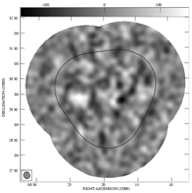
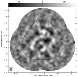
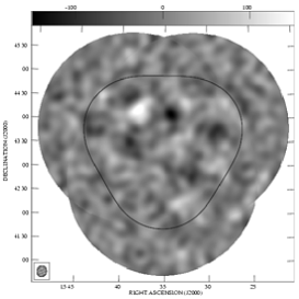
Figure 1: Mosaiced and source-subtracted maps for each of the VSA regions: left, VSA1; centre, VSA2; right, VSA3. In each case the greyscale runs from $-150$ to $150\,\mu$K and the contour indicates the half-power response of the combined primary beam.

4.1 Data checks

Table 2: Rms noise levels, in mJy beam^-1, for each of the VSA fields: the thermal noise level, $\sigma_{\rm auto}$ (measured from the autosubtracted maps – see Paper II); the noise level in the centre of each map, $\rm\sigma_{C}$; the rms CMB signal, $\rm\sigma_{CMB}$. These values are taken from CMB maps made at full resolution. The flux-to-temperature conversion is about $\rm 1\,mJy\,beam^{-1}\equiv 2.1\,\mu K$, giving mean rms CMB fluctuations in the maps of $\approx 30\,\mu$K.

Field	$\sigma_{\rm auto}$	$\rm\sigma_{C}$	$\sigma_{\rm CMB}$
VSA1E	11	19	15
VSA1F	11	19	15
VSA1G	11	15	10
VSA2E	10	19	15
VSA2F	11	22	18
VSA2G	10	23	19
VSA3E	10	18	14
VSA3F	10	20	15
VSA3G	9	14	10

As a check on the consistency of the data, we computed the $\chi^{2}$ statistic and significance for splits on the visibility data following the method described in Paper III. The significance is given as the probability to exceed the observed value in the $\chi^{2}$ cumulative distribution function. The data for each VSA field were split in two according to observing epoch and the $\chi^{2}$ values and associated significances are given in Table 3. A split between day and night observations is also included.

The consistency of the power spectra derived from each of the 3 VSA mosaiced regions was compared by forming the $\chi^{2}$ statistic on pairs of power spectra. The $\chi^{2}$ values (and significances) for the VSA1/VSA2, VSA1/VSA3 and VSA2/VSA3 power spectra comparisons are 12.2 (0.73), 9.5 (0.89) and 15.4 (0.50) respectively. In each case there are 16 degrees of freedom in the power spectrum analysis. The data sets are clearly self-consistent.

Table 3: The $\chi^{2}$ values for data splits on each of the VSA fields. In each case the visibility data from each field were split in two according to epoch and the $\chi^{2}$ of the difference vectors formed. Also tabulated are the number of degrees of freedom (DOF) and the significance of each $\chi^{2}$ value.

Field	DOF	$\chi^{2}$	Significance
VSA1E	4778	4851	0.23
VSA1F	3871	3964	0.14
VSA1G	4070	3752	0.99
VSA2E	5002	5170	0.05
VSA2F	3831	3763	0.78
VSA2G	4314	4297	0.58
VSA3E	4937	5011	0.22
VSA3F	4300	4325	0.39
VSA3G	4970	5060	0.18
Day/Night	1051	986	0.92

5 Power spectrum

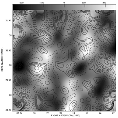
Figure 2: Comparison of the compact and extended array maps for the central part of the VSA1 field. Greyscale: Compact array map, with greyscale running from $-250$ to $250\,\mu$K. The sensitivity is nearly uniform across this area. Contours: Extended array map, contour interval $30\,\mu$K. The map has been corrected for the combined effect of the primary beams, so the noise level rises towards the edge of the map.

Figure 3: Window functions for the combined compact and extended array data set. The functions are normalised to unit area, and different bins are plotted with different linestyles.

$B$	$\ell$-range	$\ell_{h}$	$T_{0}^{2}\ell(\ell+1)C_{\ell}/2\pi[\mu{\rm K}^{2}]$
1	$100-190$	$160$	$3864_{-1141}^{+1587}$
1A	$145-220$	$190$		$4953_{-1190}^{+1538}$
2	$190-250$	$220$	$5893_{-1339}^{+1637}$
2A	$220-280$	$251$		$7031_{-1339}^{+1587}$
3	$250-310$	$289$	$5390_{-1091}^{+1289}$
3A	$280-340$	$321$		$3450_{-744}^{+942}$
4	$310-370$	$349$	$2603_{-545}^{+595}$
4A	$340-410$	$376$		$1954_{-396}^{+446}$
5	$370-450$	$416$	$1749_{-347}^{+347}$
5A	$410-475$	$431$		$1597_{-347}^{+446}$
6	$450-500$	$479$	$1638_{-496}^{+644}$
6A	$475-540$	$501$		$2675_{-545}^{+644}$
7	$500-580$	$537$	$2866_{-545}^{+595}$
7A	$540-610$	$581$		$2210_{-496}^{+644}$
8	$580-640$	$605$	$1460_{-545}^{+644}$
8A	$610-670$	$639$		$1501_{-595}^{+595}$
9	$640-700$	$670$	$2237_{-595}^{+694}$
9A	$670-725$	$696$		$2328_{-644}^{+793}$
10	$700-750$	$726$	$1922_{-744}^{+793}$
10A	$725-800$	$759$		$2905_{-644}^{+744}$
11	$750-850$	$795$	$3587_{-644}^{+644}$
11A	$800-900$	$843$		$2876_{-644}^{+694}$
12	$850-950$	$888$	$1471_{-545}^{+644}$
12A	$900-1000$	$948$		$207_{-207}^{+694}$
13	$950-1050$	$1002$	$0_{-0}^{+1091}$
13A	$1000-1125$	$1057$		$509_{-446}^{+545}$
14	$1050-1200$	$1119$	$1125_{-644}^{+694}$
14A	$1125-1275$	$1199$		$590_{-590}^{+793}$
15	$1200-1350$	$1271$	$0_{-0}^{+1431}$
15A	$1275-1525$	$1357$		$505_{-496}^{+1190}$
16	$1350-1700$	$1419$	$1311_{-1289}^{+1538}$

Table 4: The bandpowers for main and offset binnings of the complete VSA data set, combining both compact and extended array data. The $\ell$-range gives the nominal bin limits, while $\ell_{h}$ is the median value of the relevant window function. The error bars enclose 68 percent of the likelihood, even when the lower limit is zero.

$B$	${\cal C}_{B,B-2}$	${\cal C}_{B,B-1}$	${\cal C}_{B,B}$	${\cal C}_{B,B+1}$	${\cal C}_{B,B+2}$	$\mbox{Cov}_{B,B}$
$1$			$1.0$	$-0.09$	$0.012$	$17.039$
$2$		$-0.09$	$1.0$	$-0.206$	$0.021$	$22.295$
$3$	$0.012$	$-0.206$	$1.0$	$-0.114$	$0.021$	$14.886$
$4$	$0.021$	$-0.114$	$1.0$	$-0.151$	$0.031$	$3.442$
$5$	$0.021$	$-0.151$	$1.0$	$-0.227$	$0.044$	$1.316$
$6$	$0.031$	$-0.227$	$1.0$	$-0.254$	$0.047$	$3.584$
$7$	$0.044$	$-0.254$	$1.0$	$-0.268$	$0.037$	$3.912$
$8$	$0.047$	$-0.268$	$1.0$	$-0.211$	$0.09$	$4.011$
$9$	$0.037$	$-0.211$	$1.0$	$-0.406$	$0.092$	$5.135$
$10$	$0.09$	$-0.406$	$1.0$	$-0.286$	$0.055$	$7.863$
$11$	$0.092$	$-0.286$	$1.0$	$-0.187$	$0.049$	$4.883$
$12$	$0.055$	$-0.187$	$1.0$	$-0.251$	$0.079$	$3.905$
$13$	$0.049$	$-0.251$	$1.0$	$-0.336$	$0.052$	$2.353$
$14$	$0.079$	$-0.336$	$1.0$	$-0.162$	$0.03$	$5.475$
$15$	$0.052$	$-0.162$	$1.0$	$-0.196$		$6.714$
$16$	$0.03$	$-0.196$	$1.0$			$27.092$

Table 5: The correlation matrix ${\cal C}_{i,j}$ for the combined VSA data (main binning only). The values of the matrix for which ${\cal C}_{i,j}$ is not reported can be assumed to be zero. The final column gives the diagonal elements of the covariance matrix in units of $10^{5}\times\mu\rm{K}^{4}$

The fully reduced and source subtracted visibility data for the combined compact and extended VSA data sets have been analysed using the Madcow software package (Hobson & Maisinger, 2002). The typical anti-correlation between adjacent bins is $\sim 20$ percent, with one as high as $40$ percent. We use variable sized bins to reflect the differences in density of coverage of the aperture plane, but also repeat the calculation with bin centres shifted by half a bin width in order to sample effectively the features of the power spectrum. We follow the procedure outlined in Paper III to determine the window function $W(\ell)$ which determines how each bin samples the underlying power spectrum. The window functions for our analysis are shown in Figure 3. The resulting power spectrum is shown in Figure 5, numerical values for both binnings are given in Table 4 and the correlation matrix for the main binning in Table 5. The bin centres given in each case are the medians of the respective window functions rather than the nominal bin centres.

There is a systematic uncertainty of 7 percent in the scaling of the power spectrum due to the uncertainty in the effective temperature of the primary calibration source, Jupiter. The error in flux density to temperature conversion (equivalent to the beam uncertainty in scanned-beam experiments) is negligible.

6 Discussion & conclusions

We have measured the power spectrum of the CMB over the multipole range $\ell=160$ – $1400$ using two configurations of the VSA. The combined power spectrum clearly shows three peaks, a sharp fall-off in power above $\ell~{}\sim~{}800$, and marginal evidence for a fourth peak. Figure 5 shows the VSA data plotted alongside that from other recent CMB experiments: there is excellent agreement between all the experiments.

To quantify the significance of these peaks in the power spectrum, we used a model of five Gaussians parametrised by their amplitude, position and width, as described in Ödman et al. (2002). We analysed the VSA data alone, plus two data sets consisting of a compilation of recent data, and used an MCMC routine to constrain the parameters simultaneously. In Table 6, we list the constraints on the amplitudes and positions of the first four peaks after marginalising over their widths (there are no interesting constraints on the fifth peak). Including the new VSA measurement improves the constraints on the amplitude of the fourth peak, as well as confirming the detection of the first three peaks.

Fits of adiabatic inflationary model power spectrum, with associated estimates of cosmological parameters, are presented in a companion paper (Slosar et al., 2002).

In our current observing configuration we are increasing the size of the mosaiced regions and also observing new regions; this will increase both the sensitivity and $\ell$-resolution of the power spectrum. We also plan to increase the $\ell$-range of the VSA using larger antennas and longer baselines to study further peaks in the primordial spectrum and give information on the region where CBI observes excess power (Mason et al., 2002).

Band powers, correlation matrices and window functions can be downloaded from
http://mrao.cam.ac.uk/telescopes/vsa/results.html

Table 6: Constraints on parameters of a multiple Gaussian fit to the power spectrum data. The inclusion of the new VSA data places constraints on the power beyond the first three peaks. Dataset I consists of the QMASK compilation (Xu et al., 2002), MSAM (Wilson et al., 2000), Python V (Coble et al., 2001), Boomerang 98 (Netterfield et al., 2002), Maxima (Lee et al., 2001), DASI (Halverson et al., 2002), CBI (Pearson et al., 2002), Archeops (Benoit et al., 2002) and the VSA data from the compact array configuration. Dataset II is identical, except for the inclusion of the new VSA data. Note that, while the lack of a lower bound on a $\Delta$T implies a significant contribution to the power from adjacent Gaussians, narrow constraints on peak locations imply strong evidence for spectral features rather than a flat spectrum of excess power.

	VSA only	dataset I	dataset II
$\Delta T_{1}$	$71.4_{-5.5}^{+11.3}$	$70.2_{-2.0}^{+2.1}$	$71.7_{-2.1}^{+2.0}$
$\Delta T_{2}$	$45.5_{-5.6}^{+6.4}$	$38.5_{-7.8}^{+8.1}$	$42.3_{-10.4}^{+4.7}$
$\Delta T_{3}$	$47.0_{\mbox{\tiny unbounded}}^{+8.9}$	$42.5_{-2.2}^{+1.5}$	$43.3_{-2.3}^{+1.7}$
$\Delta T_{4}$	$25.9_{\mbox{\tiny unbounded}}^{+14.1}$	$18.0_{\mbox{\tiny unbounded}}^{+19.1}$	$19.6_{-11}^{+11.7}$
$\ell_{1}$	$224_{-28}^{+11}$	$214_{-5}^{+4}$	$216_{-6}^{+3}$
$\ell_{2}$	$509_{-84}^{+81}$	$511_{-16}^{+12}$	$510_{-14}^{+11}$
$\ell_{3}$	$771_{-70}^{+55}$	$786_{-48}^{+29}$	$782_{-52}^{+23}$
$\ell_{4}$	$1171_{-205}^{+67}$	$1260_{-321}^{+37}$	$1157_{-118}^{+167}$

Figure 4: Combined CMB power spectrum from the three mosaiced VSA fields. The error-bars represent $1\sigma$ limits; the two sets of data points correspond to alternative interleaved binnings of the data.

Figure 5: A comparison of the VSA data (filled circles) with results from the BOOMERANG (open squares), MAXIMA (open circles), DASI (open triangles) and CBI (stars) experiments. Two sets of error bars are plotted for each data set; the smaller (inner) of the two indicate only random errors, whilst the larger bars indicate the amount by which the inner points could move due to absolute calibration and beam uncertainty. In each case the error bars indicate $1\sigma$ limits.

References

- Anderson et al. (1991) Anderson M., Rudnick L., Leppik P., Perley R., Braun R., 1991, ApJ, 373, 146
- Benoit et al. (2002) Benoit A., et al., 2002, The Cosmic Microwave Background Anisotropy Power Spectrum measured by Archeops, submitted to A&A Letter
- Bietenholz et al. (1991) Bietenholz M. F., Kronberg P. P., Hogg D. E.and Wilson A. S., 1991, ApJ, 373, L59
- Coble et al. (2001) Coble K., et al., 2001, Cosmic Microwave Background Anisotropy Measurement From Python V, submitted to ApJ
- Giardino et al. (2001) Giardino G., Banday A. J., Fosalba P., Górski K. M., Jonas J. L., O’Mullane W., Tauber J., 2001, A&A, 371, 708
- Green (2002) Green D. A., 2002, in ASP Conf. Ser. 271: Neutron Stars in Supernova Remnants The Crab Nebula at 850 microns. p. 153
- Halverson et al. (2002) Halverson N. W., et al., 2002, ApJ, 568, 38
- Hobson & Maisinger (2002) Hobson M. P., Maisinger K., 2002, MNRAS, 334, 569
- Lee et al. (2001) Lee A. T., et al., 2001, Astrophys.J., 561, L1
- Mason et al. (2002) Mason B. S., et al., 2002, The Anisotropy of the Microwave Background to l = 3500: Deep Field Observations with the Cosmic Background Imager, submitted to ApJ
- Mason et al. (1999) Mason B. S., Leitch E. M., Myers S. T., Cartwright J. K., Readhead A. C. S., 1999, AJ, 118, 2908
- Netterfield et al. (2002) Netterfield C. B., et al., 2002, ApJ, 571, 604
- Ödman et al. (2002) Ödman C. J., Melchiorri A., Hobson M. P., Lasenby A. N., 2002, Constraining the shape of the CMB: a Peak-by-Peak analysis, submitted for publication in MNRAS
- Padin et al. (2002) Padin S., et al., 2002, PASP, 114, 83
- Pearson et al. (2002) Pearson T. J., et al., 2002, The Anisotropy of the Microwave Background to l = 3500: Mosaic Observations with the Cosmic Background Imager, submitted to ApJ
- Peebles & Yu (1970) Peebles P. J. E., Yu J. T., 1970, ApJ, 162, 815
- Sakharov (1965) Sakharov A. A., 1965, ZhETP, 49, 345
- Scott et al. (2002) Scott P. F., et al., 2002, First results from the Very Small Array III: The CMB Power Spectrum, accepted for publication in MNRAS
- Silk (1968) Silk J., 1968, ApJ, 151, 459
- Slosar et al. (2002) Slosar A., et al., 2002, Cosmological parameter estimation an Bayesian model comparison using VSA data, submitted for publication in MNRAS
- Sunyaev & Zel’dovich (1970) Sunyaev R., Zel’dovich Y., 1970, Comments Astrophys. Space Phys., 2, 66
- Taylor et al. (2002) Taylor A. C., et al., 2002, First results from the Very Small Array II: observations of the CMB, accepted for publication in MNRAS
- Tegmark et al. (2000) Tegmark M., Eisenstein D. J., Hu W., de Oliveira-Costa A., 2000, ApJ, 530, 133
- Waldram et al. (2002) Waldram E. M., Pooley G. G., Grainge K. J. B., Jones M. E., Saunders R. D. E., Scott P. F., Taylor A. C., 2002, A Survey of Radio Sources at 15 GHz with the Ryle Telescope: Techniques and Properties, submitted to MNRAS
- Watson et al. (2002) Watson R. A., et al., 2002, First results from the Very Small Array I: observational methods, accepted for publication in MNRAS
- Wilson et al. (2000) Wilson G. W., et al., 2000, ApJ, 532, 57
- Xu et al. (2002) Xu Y., Tegmark M., de Oliveira-Costa A., 2002, Phys.Rev.D, 65, 83002