Rotation and outflow in the central kiloparsec of the water-megamaser galaxies IC 2560, NGC 1386, NGC 1052, and Mrk 1210

Optical emission-line profiles were evaluated in order to explore the structure of galactic nuclei containing H₂O megamaser sources. Long-slit spectra of IC 2560, NGC 1386, NGC 1052 and Mrk 1210 were obtained at $\sim 100$ km/s spectral and $\sim 2\arcsec\times 2\arcsec$ spatial resolution. The following individual properties of the objects were found: The active nucleus of IC 2560 (innermost $\pm 2\arcsec$) emits lines typical for a high-ionization Seyfert-2 spectrum albeit with comparatively narrow profiles (FWHM $\sim 200$ km/s). Line wings are stronger on the blue side than on the red side suggesting outflow. The central velocity gradient fits into the general velocity curve of the galaxy. Attributing it to a rotating disk coplanar with the galaxy leads to a Keplerian mass of $\sim 10^{7}$ M_⊙ inside a radius of 100 pc. — The central 6″ sized structure seen on HST H$\alpha$ and [Oiii] images of NGC 1386 appears to be the inner part of a near-edge-on warped rotating spiral disk that is traced in H$\alpha$ within a diameter of 17″ along p.a. 23°. This interpretation is based on observed kinematic continuity and a typical S-shaped dust lane crossing the kinematical center. The central velocity gradient yields a Keplerian mass estimate of $\sim$10⁸ M_⊙ inside $R=100$ pc and 5 10⁹ M_⊙ inside 0.8 kpc. The total mass of the ionized gas of $10^{5-6}$ M_⊙ is small compared to the dynamical mass of the spiral disk. — The kinematical gradient of the rotating gas disk in the center of the elliptical galaxy NGC 1052 yields a mass of $\sim$6 10⁸ M_⊙ inside 166 pc. Two components are found: component $\cal A$ arises in a rotating disk, component $\cal B$ is blueshifted by $\sim 400$ km/s relative to the disk. $\cal B$ likely originates from outflowing gas distributed within a wide cone. There is no need for a broad H$\alpha$ component in unpolarized flux. The peculiar polarization seen in [Oi]$\lambda 6300$ by Barth et al. (1999) may be related to the outflow component. — In Mrk 1210, a redshifted component $\cal R$ contributes to the exceptional width of [Oi]$\lambda 6300$. An additional blueshifted component $\cal B$ strong in [Oiii] allows to fit the H$\alpha$ + [Nii] blend without a broad component of H$\alpha$. $\cal B$ and $\cal R$ are likely to be outflow components. The location of the brightness maximum BM is slightly ($\sim 1\arcsec$) shifted relative to the kinematical center KC. Locating the true obscured nucleus in KC makes it understandable that BM displays faint broad scattered H$\alpha$ in polarized light. — Galactic rotation and outflow of narrow-line gas are common features of this sample of water-megamaser galaxies. All decomposed line-systems exhibit AGN typical line ratios. Recent detections of H₂O megamasers in starburst galaxies and the apparent asssociation of one megamaser with a Seyfert 1 AGN suggest that megamasers can possibly be triggered by optically detectable outflows. The frequently encountered edge-on geometry favoring large molecular column densities appears to be verified for NGC 1386 and IC 2560. For NGC 1052 and Mrk 1210, maser emission triggered by the optically detected outflow components cannot be ruled out.

1 Introduction

During the past two decades, powerful H₂O masers have been detected in the 6₁₆–5₂₃ transition at 22 GHz ($\lambda$$\sim$1.3 cm) towards almost thirty galaxies known to contain an active galactic nucleus (AGN) of Seyfert 2 or LINER type (dos Santos & Lépine 1979; Gardner & Whiteoak 1982; Claussen et al. 1984; Henkel et al. 1984, 2002; Haschick & Baan 1985; Koekemoer et al. 1995; Braatz et al. 1994, 1996, 1997; Greenhill et al. 1997a, 2002, 2003; Hagiwara et al. 1997; Falcke et al. 2000). These H₂O masers (hereafter ‘megamasers’) appear to be more luminous, by orders of magnitude, then the brightest H₂O masers observed in galactic star forming regions. All interferometric data of H₂O megamasers point toward a nuclear origin. The emission originates from the innermost parsec(s) of the parent galaxy (e.g. Claussen & Lo 1986; Greenhill et al. 1995b, 1996, 1997b; Miyoshi et al. 1995; Claussen et al. 1998; Trotter et al. 1998; Herrnstein et al. 1999). Adopting the so-called unified model (Antonucci & Miller 1985; Antonucci 1993) with Seyfert 2 nuclear disks being viewed edge-on, megamaser activity must be related to large column densities along the line of sight, a picture in line with the presence of dense molecular gas.

There exist at least two different classes of megamasers, those forming a circumnuclear disk (like in NGC 4258) and those associated with nuclear jets (e.g. NGC 1052). The observed H₂O transition traces a dense ($\ga$10⁷ cm^-3) warm ($T_{\rm kin}$$\ga$400 K) molecular medium. The additional presence of jets and a nuclear X-ray source requires, however, the coexistence of neutral and ionized gas in the nuclear regions of these galaxies. In an attempt to study connections between megamaser emission on milliarcsecond scales and optical phenomena on arcsecond scales, here we present and analyze optical emission line spectra from four megamaser galaxies.

Table 1: Journal of the spectroscopic observations

Object/helioc. corr.	Frame	Date (beg.)	p.a. (slit)	Pos. of slit	$\lambda$ range (Å)	Exp.time (s)
NGC 1052	F020	11-Jan-96	90°	through nucleus	5400-7400	3600
$-27$ km/s	F056	12-Jan-96	90°	through nucleus	5400-7400	1800
	F057	12-Jan-96	90°	2″ south of nucleus	5400-7400	1800
	F058	12-Jan-96	90°	2″ north of nucleus	5400-7400	1800
	F078	13-Jan-96	45°	through nucleus	5000-6800	3600
	F107	14-Jan-96	45°	through nucleus	4000-6000	3600
	F108	14-Jan-96	45°	2″ northwest of nucleus	4000-6000	3600
NGC 1368	F023	11-Jan-96	90°	through nucleus	5400-7400	3600
$-17$ km/s	F026	11-Jan-96	90°	2″ north of nucleus	5400-7400	3600
	F080	13-Jan-96	23°	through nucleus	5000-6800	2700
	F112	14-Jan-96	23°	through nucleus	4000-6000	3600
Mrk 1210	F066	12-Jan-96	90°	through nucleus	5400-7400	3600
$+6$ km/s	F084	13-Jan-96	90°	through nucleus	5000-6800	1333
	F085	13-Jan-96	90°	2″ south of nucleus	5000-6800	3600
	F087	13-Jan-96	90°	2″ north of nucleus	5000-6800	3600
	F116	14-Jan-96	90°	through nucleus	4000-6000	3600
IC 2560	F030	11-Jan-96	90°	through nucleus	5400-7400	3600
$+20$ km/s	F118	14-Jan-96	90°	through nucleus	4000-6000	3600

2 Data acquisition

The spectra were obtained in January 1996 using the Boller & Chivens spectrograph attached to the Cassegrain focus of the ESO 1.52 m spectrographic telescope. A log of the observations, in particular the observed wavelength ranges, are given in Table 1. The detector was La Silla CCD No. 24 (FA2048L CCD chip with 15 $\mu$m wide square pixels). The spatial resolution element is 0$\aas@@fstack{\prime\prime}$68 px^-1. Seeing and telescope properties limited the spatial resolution to the range 1$\aas@@fstack{\prime\prime}$2 – 2$\aas@@fstack{\prime\prime}$5 which was determined by the width of standard star spectra on the focal exposures. The slit was visually centered and guided on the nuclear brightness maximum or a nearby offset star. The 2″ wide slit projects to a spectral resolution of $\sim 2$Å  ($\sim 100$ km s^-1) as is confirmed by the full width at half-maximum (FWHM) of comparison lines and the [Oi]$\lambda 6300$ night sky line.

Employing the ESO MIDAS standard software (version Nov. 96) the CCD frames were bias subtracted and divided by well exposed flat-field frames. Night-sky spectra ‘below’ and ‘above’ any notable galaxy emission were interpolated in the region of the galactic spectrum and subtracted in each case. From such cleaned frames either single rows (corresponding to 0$\aas@@fstack{\prime\prime}$68 and 2″ along and perpendicular to the slit direction, respectively) or the averages of two adjacent spectral rows ($1\aas@@fstack{\prime\prime}36\times 2\arcsec$ formal spatial resolution) were extracted.

Tüg’s (1977) curve was used to correct for atmospheric extinction. The spectra were flux calibrated using the standard star 40 Eri B (Oke 1974), but we use the calibration only for relative line ratios due to occasional thin cirrus. Forbidden-line wavelengths were taken from Bowen (1960). Spectra in the blue and red region of the bright elliptical NGC 3115 were taken as well and we used them as templates to subtract the stellar contribution from those spectra in which we analyzed the line-profile structure and intensity ratios.

3 General data and morphology

Table 2 (column 2) exhibits the morphological diversity of the four galaxies although we only refer to the crude Hubble type. While NGC 1052 is an elliptical galaxy (Fosbury et al. 1978), NGC 1386 (Sa according to Weaver et al. 1991) and IC 2560 (Sb in Fairall 1986; SBb in Tsvetanov & Petrosian 1995) are disk systems whereas Mrk 1210 is hard to classify from ground-based data. It looks roundish with an amorphous body supplemented by a few shell-like features, possibly a late-stage merger (Heisler & Vader 1994). An HST-snapshot image unveils a kpc-sized central spiral apparently seen close to face-on that can be classified as Sa in a Hubble scheme (Malkan et al. 1998), although it should be cautioned that this spiral may be gaseous rather than a density-wave triggered stellar spiral.

Column 3 gives the heliocentric value of the systemic velocity as derived from our data. All velocity values given below are heliocentric. Column 4 of Table 2 gives distances (see footnotes) in accordance with recent work to ease comparison. Column 5 gives the linear scale in the galaxy applicable along the major axis for the distance (col. 4) assumed. Cols. 6 and 7 give the position angle of the apparent major axis and the angle of inclination from face-on. For the present work, these numbers should preferably correspond to the disk in which emission lines are generated, which is, however, only poorly determined. Comments and footnotes explain the origin of the numbers given.

4 Results on individual galaxies

Details of the spectral data analysis to find clues for basic kinematical bulk components in the shape of the emission lines are outlined in Appendices A – B (treatment of individual spectra) and Appendix C (determination of rotation curves). Here we discuss our results, starting with the two strongly inclined spiral galaxies IC 2560 and NGC 1386. Then we turn to the apparently more complex spectra of NGC 1052 and Mrk 1210.

4.1 The Seyfert IC 2560

Table 2: Adopted basic data of the four galaxies ($v_{\rm hel}$ from this work)

Object	Type	$v_{\rm hel}$	dist.	lin. sc.	maj. ax.	inclin.	Comment
Coord.(1950)	Hubble	km s-1	Mpc	pc/″	°	°
NGC 1052	E	$1462\pm 20$	17.1	82.9	49	$\sim 60$	p.a. (major axis) and inclination
0238-08							of nuclear gas disk
NGC 1386	Sa	$878\pm 20$	19.8	96.0	23	74	major axis and inclination of galaxy
0334-36							on large scale (Tully 1988)
Mrk 1210	amorph	$4022\pm 30$	53.6	260.0	$\approx 110$	$\approx 0$	maj. ax. from gas kinematics; inclin. from image
0801+05	Sa						of kiloparsec spiral (Malkan et al.  1998)
IC 2560	SBb	$2922\pm 20$	26	126.1	45	63	p.a. and inclination of galaxy; distance
1014-33							39 Mpc if peculiar motion is ignored

4.1.1 Kinematics

Along p.a. (90°, 270°) we traced regions with emission lines 22″ east until 50″ west. The reference position 0″ on the abscissa of Fig. 1 marks the spot where the maximal intensity of nuclear line emission is reached. Here $v_{\rm hel}^{\rm c}=(2922\pm 20$) km/s is measured, which we identify with the systemic velocity. Outside the innermost nuclear region (useful line measurements are possible from the nuclear maximum within a diameter of 5″) appears a gap with no traces of a line and emission lines further out originate in disk HII regions. The corresponding velocity curve is shown in Fig. 1. Between 15″ and 20″ west an interesting local up- and downturn (presumably density-wave related) can be noted in the spiral arm. This and two other intersections of a spiral arm ($\sim$ 45″ to 50″ west and 17″ to 22″ east) exhibit contiguous H$\alpha$ emission and mostly [Nii] as well, with each region a few hundred parsec in extent.

To evaluate the central linear gradient a deprojection onto the plane of the galaxy is required. Here $\theta=45\degr$ is the angle in the plane of the sky between slit position and major axis, because the slit extends along p.a. 90° and the galaxy’s major axis along 45°, while its inclination $i=63\degr$ (Table 2).

Altogether, a nuclear gradient in rotational velocity of $20$ km/s/(100 pc) is obtained yielding a Keplerian mass estimate ($M=Rv^{2}/G$) of $M_{100}$ = 9.3 10⁶ M_⊙ within a nuclear radius $R=100$ pc. This is only 2.6 times the value that Ishihara et al. (2001) obtain for the mass inside the central 0.07 pc (note that they assumed an edge-on disk). Extrapolating our gradient to this radius yields a negligible velocity compared to the actual velocities of the maser sources (210–420 km/s) measured by Ishihara et al. (2001) between 0.07 and 0.26 pc. This might be explained by an inner Keplerian upturn of the rotation curve due to the central mass concentration.

The line profiles from the nuclear region within $\pm 2\arcsec$ of the center (defined by the maximum of continuum and line brightness) are relatively narrow for a Seyfert, with FWHMs of (200–250) km/s. Fig. 2 shows that the blue side of the [Oiii] profiles can be fit by a Lorentzian while Fig. 3 shows that the red side of the [Oiii] profiles can be fit by a Gaussian (this also holds for H$\beta$, H$\alpha$ and [Nii]). This indicates that the observed [Oiii] profiles have a stronger outer wing on the blue side, which is most likely a signature for outflow. However, the amount and velocity of the outflow cannot be modelled precisely because the line width is only twice our spectral resolution. Taking the Gaussian as representative for the rotational component convolved with the instrumental profile, the deconvolved l.o.s. outflow-velocity component is estimated to be $\sim 100$ km/s.

It should be noted that our near-edge-on view of the central kpc-disk may be unfavorable to measure outflowing gas, because outflow is frequently directed perpendicular to a galactic disk.

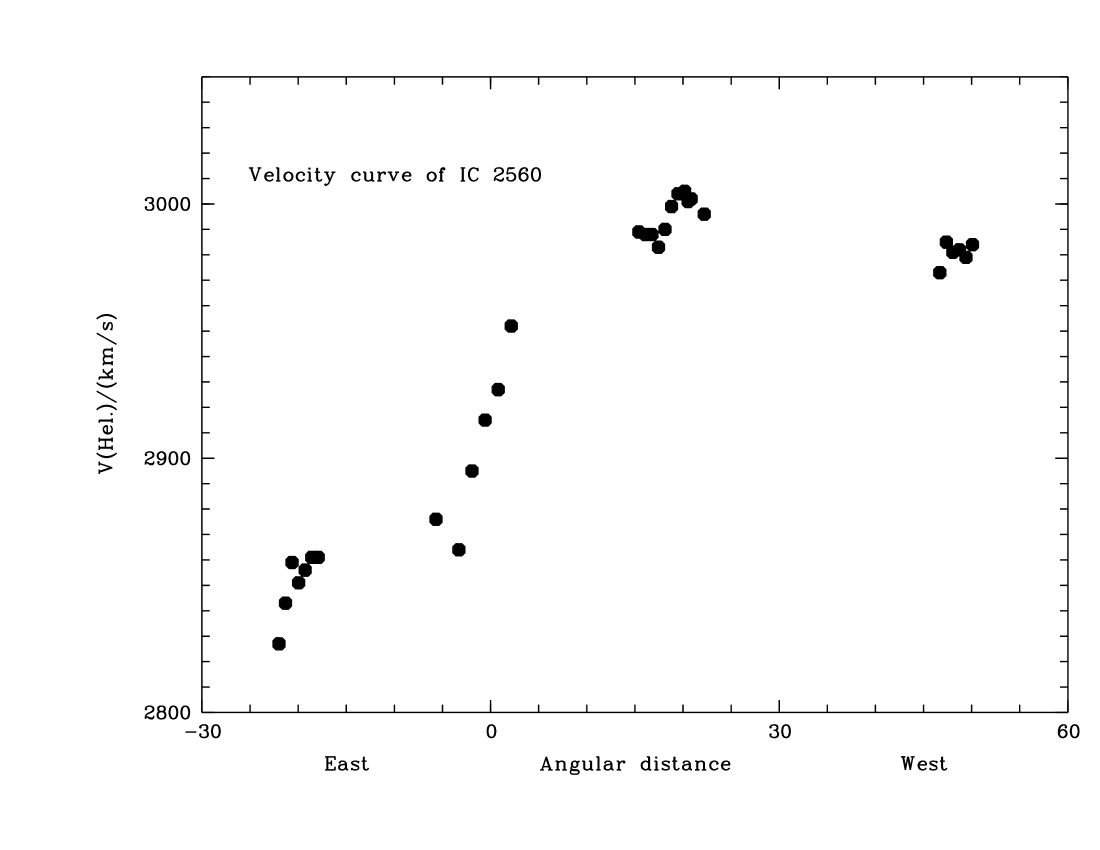
Figure 1: Heliocentric radial velocities (averages of the peaks of H$\alpha$ and [Nii]$\lambda 6583$) measured in spectrum F030 of IC 2560 (along p.a. 90°; abscissa in arcsec). Statistical uncertainty $\pm 11$ km/s.

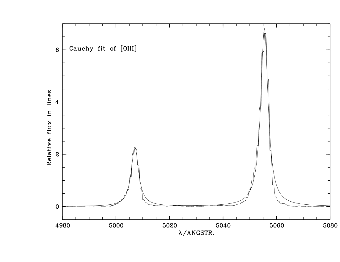
Figure 2: [Oiii]$\lambda\lambda 4959,5007$ from the central 1$\aas@@fstack{\prime\prime}$36 (E-W) $\times$ 2″(N-S) of IC 2560 (F118) (plotted in the observed frame as all subsequent spectra). The Lorentzians used for the fits are too wide within the red wings.

Figure 3: The same [Oiii]$\lambda\lambda 4959,5007$ observations as in Fig. 2, but now fit by Gaussians, which turn out to be too narrow to fit the blue wings.

4.1.2 Trends in line-ratios

For readers interested in line-excitation variations a few trends of line ratios are given in the present, albeit primarily kinematic, study. In the innermost $\pm 2\arcsec$  along p.a. (90°, 270°) the intensity ratios of [Nii]/H$\alpha$ and [Sii]/H$\alpha$ are increasing to the west. At the three positions, central maximum, 1″ west, and 2″ west, we measure: [Oi]$\lambda 6300$/H$\alpha=$ 0.15, 0.2 and ‘not measurable’; [Nii]$\lambda 6583/$H$\alpha=$ 1.05, 1.2 and 1.5; [Sii]($\lambda 6716+\lambda 6731)/$H$\alpha=$ 0.6, 0.65 and 0.9, respectively. [Oiii] was extracted over 2″ bins yielding [Oiii]$\lambda 5007/$H$\beta=13$ in the central bin, which decreases to 10.5 at 2″ west, while it may slightly increase to 14 at 2″ east. The other line ratios at 1″ east and 2″ east do not significantly differ from the central values. The density-indicator [Sii]$\lambda 6716$/[Sii]$\lambda 6731$ is found in the range $0.90\pm 0.05$ in this inner region, corresponding to single-component densities in the range $(7-10)\,10^{2}$ cm^-3.

The relative strengthening of the low-ionization lines to the west (which is also the far side if the spiral is trailing) may be due to a decrease of the ionization parameter by increased filtering of the ionizing radiation with nuclear distance. Such an effect is demonstrated in Schulz & Fritsch (1994). The directly measured line intensities of H$\alpha$ have a steeper fall-off to the west than to the east.

Exploratory spectra with an east-west oriented slit positioned 2″, 4″ and 6″ south of the nucleus (taken to look for some circumnuclear influence of the activity) are too weak for detailed measurements. At 4″ south the spectrum appears to be of lower excitation than known from the standard LINER sample shown in the diagnostic diagrams of Schulz & Fritsch (1994).

4.2 The Seyfert NGC 1386

4.2.1 Global kinematics of the inner emission-line region

We here first describe a velocity curve derived from the line peaks of H$\alpha$ and [Nii]$\lambda 6583$ measured along the large-scale major axis at p.a. 23° (Fig. 4). The [Oiii]$\lambda\lambda 4959,5007$ (spectrum F112) peak positions agree in the innermost $\pm 3\arcsec$ where they can be measured. For a comparison of the complicated line profiles of [Oiii] and H$\alpha$ see Sect. 4.2.2. H$\beta$ is faint, partially due to strong extinction (Sect. 4.2.2), and cannot be measured beyond $\sim 2\aas@@fstack{\prime\prime}5$ of the brightness maximum.

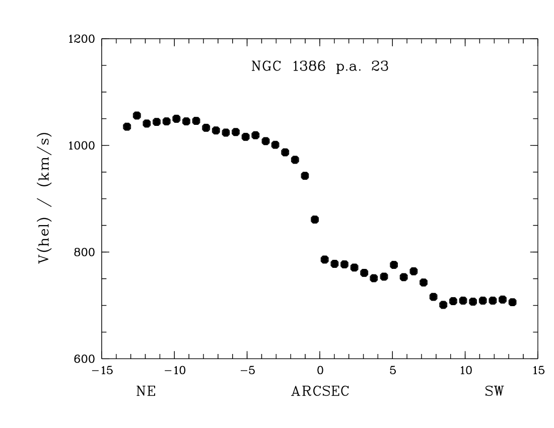
Figure 4: Velocity curve of NGC 1386 along p.a. 23°(from F080). The data correspond to the mean position of the line peaks of H$\alpha$ and [Nii]$\lambda 6583$ in the raw spectrum.

The zero point of the abscissa of Fig. 4 corresponds to the spectral row where continuum and intensities of H$\alpha$ and [Oiii] are at maximum. We call this brightness maximum ‘region $\cal{B}$’ because of its blueshift relative to the kinematical center KC (see Fig. 4). KC is defined by taking the symmetry center of the outer portions of the velocity curve. For its determination we took means of the flat portions of the velocity curve beyond $\pm 8\arcsec$  yielding (after symmetrizing) $v=168$ km/s (northeast) and $v=-168$ km/s (southwest) around $v_{\rm KC}=877$ km/s. Below in Sect. 4.2.2 we will find that the mean of the line cores of six different lines arising within the innermost 2″ of KC yields 878 km/s, which is in (fortuitously) perfect agreement with $v_{\rm KC}$.

Linearly interpolating in the spatial direction, KC is found to lie $-0\aas@@fstack{\prime\prime}6$ (to the northeast) offset from $\cal{B}$.

The position of $\cal{B}$ on the sky can be inferred from an HST H$\alpha$ image shown in Ferruit et al. (2000) (their Fig. 4, left panel, middle row; hereafter FWM2000). The following description refers to their H$\alpha$ image. Our spectrograph’s slit encompasses the bright parts of the image by a 2″ wide band along p.a. 23°. The major axis of the H$\alpha$ emission string appears to extend along p.a. 6°, or $\Delta\theta=17\degr$ offset from the slit position angle.

From the rotation pattern and the appearance of NGC 1386 as a highly inclined galaxy one expects to look upon a similarly inclined emission-line disk in the center. Images of galaxies at high inclination commonly show a midplane-dust lane. In FWM2000’s H$\alpha$ image appears indeed a dark lane crossing the center between the two brightest spots that seems to wind from the southwest to the northeast in a extended S-shaped pattern.

The dominating spot in FWM2000’s image, just below the dust lane, has to coincide with $\cal{B}$. $\cal{B}$ is located at the zero position in our Fig. 4. The kinematical center KC, offset by 0$\aas@@fstack{\prime\prime}$6 in our spectrum, has to be located within the dust lane.

The H$\alpha$ image structure is characteristic for a near-to-edge-on and warped two-armed spiral disk. The spiral bending is in the same sense as that of the large galaxy, but the inclination appears to be larger than $i=74\degr$, the inclination of the large scale disk (Table 2). Since the northeastern part is receding, the northwestern arm should be on the near side if we make the usual assumption that the arms are trailing.

The above interpretation of the main extended structure in FWM2000’s H$\alpha$ image may be considered to be at variance with the usual notion of a ‘radiation cone along the minor axis’. When interpreting IR spectroscopy, Reunanen et al. (2002) use the term ‘radiation cone’ to describe the morphology of the emission-line gas, but, on the other hand, they note that the H₂ “rotation curve is relatively ordered parallel to the cone, suggesting that circular motions dominate the kinematics”. Our data agree with this statement on the kinematics, but it is not clear whether the edge-on disk is ionized by a UV ‘radiation cone’ (small plumes along p.a. $90^{\circ}$ could be due to outflowing gas illuminated by a radiation cone; see end of Sect. 4.2.2).

The interpretation in terms of dominating circular motions of the inner ionized gas is further supported by kinematical continuity with gas at larger galactocentric distances. The bright H$\alpha$ features seen between 4″ northeast and 2″ southwest in the HST image are kinematically smoothly joined with gas further out (that is traced in our spectra but not in the HST image) to 14″ northeast and to 14″ southwest (Fig. 4). Furthermore, the map of peak velocities in Weaver et al. (1991; their Fig. 5) shows a slightly distorted, but nonetheless typical pattern of a rotating disk. An interpretation by a bipolar flow accidentally aligned with the kinematical major axis of the rotating disk would appear contrived, because it had to be essentially decoupled from the gravitational field and its accordingly stratified interstellar medium.

Altogether, the natural explanation of our Fig. 4 is that of a slightly projected rotation curve, although the rotating rings may not have a common plane, because FWM2000 noted changes of ellipticity and p.a. (major axis) with galactocentric radius. Owing to its AGN-typical line ratios the H$\alpha$ gas is ionized by nuclear AGN radiation, but since the disk is likely to be matter-bounded the UV radiation is not necessarily confined to a narrow cone. Therefore we dismiss the term ‘radiation cone’ for NGC 1386.

For estimates of the rotation velocity utilizing Eq. 3 we have to know the orientation of the supposed single disk. Regarding apparent distances a projection correction would be small (because $\cos 17\degr=0.96$). A velocity correction with $i=74\degr$ and $\theta=17\degr$ would formally yield a factor 1.5 to obtain a rotational velocity. However, this procedure is questionable because $i=74\degr$ corresponds to the outer galactic disk and the inner disk addressed here appears to be more inclined.

For Keplerian mass estimates (that are good to a factor of two even if the potential is flattened; cf. Lequeux 1983) it is therefore sufficient to assume that the slit extends along the major axis and that the disk is seen edge-on, i.e. measured velocities are rotational velocities and angular distances along the slit correspond directly to linear distances (an inclination correction solely with $\sin 74\degr$ would lead to 8% larger masses).

The HST image (FWM2000’s Fig. 4) only shows the inner 6″ of the disk where H$\alpha$ is brightest. As noted above, the velocity curve in our Fig. 4 extends into the galactic disk beyond the bright H$\alpha$ clouds seen in the HST image. The curve becomes flat at $\pm 8\aas@@fstack{\prime\prime}5$ corresponding to a galactocentric radius $R=816$ pc at which $v=168$ km/s. These numbers yield a mass of $M=Rv^{2}/G=5.4\,10^{9}$ M_⊙ in the central region of 1.6 kpc diameter of NGC 1386. In the center, the steep rise of the rotation curve to $\sim 90$ km/s at 1″ yields a mass of $1.8\,10^{8}$ M_⊙ within a diameter of 200 pc.

From the observed H$\alpha$ luminosity $L_{{\rm H}\alpha}\approx 10^{40}$ erg/s (Colbert et al. 1997) and adopting $L_{{\rm H}\alpha}=2.9\ L_{{\rm H}\beta}$  one can estimate the volume emission measure $Vn_{e}^{2}$ for fully ionized ($n_{e}=n_{p}$, the proton density) hydrogen gas via $L_{{\rm H}\beta}=(Vn_{e}^{2})(4\pi j_{{\rm H}\beta}/n_{e}^{2})$ ($j_{{\rm H}\beta}$ is the emission coefficient of H$\beta$ per steradian). Taking from Osterbrock (1989; Table 4.2) $4\pi j_{{\rm H}\beta}/(n_{e}n_{p})=1.24\,10^{-25}$ erg cm³ s^-1 (for $T=10^{4}$ K) and adopting a typical NLR electron-density range $n_{e}=10^{2-3}$ cm^-3, applying a conservative extinction correction of a factor of 3 and a factor of 1.45 for the presence of helium, one obtains $10^{5-6}$ M_⊙ for the mass of line-emitting gas, which is small compared to the dynamical masses given above.

4.2.2 Line profiles from the inner disk

For sampling in closer accordance with the seeing we binned pairs of the 0$\aas@@fstack{\prime\prime}$68 wide CCD rows to spectral scans, which each encompass light from 1$\aas@@fstack{\prime\prime}$36 along the entrance slit, and subtracted scaled spectra of our template NGC 3115 to remove the contribution of stellar light. H$\beta$ turned out to be faint and too noisy for an accurate estimate of the extinction from the Balmer decrement. Roughly, at the position of the line maximum we have $I$(H$\alpha$)/$I$(H$\beta$) $\approx 4$, while this value approaches 6 at 1$\aas@@fstack{\prime\prime}$36 southwest, and 7 at 1$\aas@@fstack{\prime\prime}$36 northeast. In a simple screen model these values translate into $A_{\rm V}=0\aas@@fstack{m}9$, $2^{m}$ and 2$\aas@@fstack{m}$5, respectively.

Figs. 5 and 6 show the ‘blue’ line profiles of [Oiii], and Figs. 7 and 8 display the ‘red’ line profiles of H$\alpha$ and [Nii] from the ‘central’ (max. line emission) 1$\aas@@fstack{\prime\prime}$36 along the slit and the next two 1$\aas@@fstack{\prime\prime}$36 wide bins towards the southwest (p.a. (23°+ 180°)) and towards the northeast (p.a. 23°), respectively. Although the blue and red frames were exposed at 1$\aas@@fstack{\prime\prime}$4 and 2$\aas@@fstack{\prime\prime}$5 seeing, respectively, the profiles of [Oiii] on one side and H$\alpha$ or [Nii] on the other side reveal the same basic shape. The most pronounced difference appears at 1$\aas@@fstack{\prime\prime}$36 southwest, the sharp shoulders on the red side of [Oiii] are smoothed out in H$\alpha$ and [Nii], which we trace back to the seeing effect.

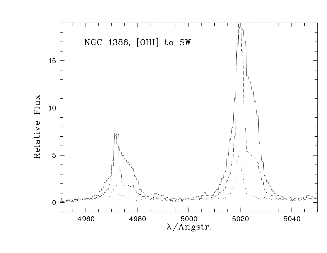
Figure 5: [Oiii]$\lambda 4959$ and $\lambda 5007$ line profiles extracted from 1$\aas@@fstack{\prime\prime}$36 wide spectral scans (of spectrum F112). Continuous line: from region $\cal{B}$ (line maximum); dashed: 1$\aas@@fstack{\prime\prime}$36 southwest; dotted: 2$\aas@@fstack{\prime\prime}$72 southwest.

Figure 6: As in Fig. 5, but now towards northeast. Continuous line: from region $\cal{B}$ (line maximum); dashed: 1$\aas@@fstack{\prime\prime}$36 northeast; dotted: 2$\aas@@fstack{\prime\prime}$72 northeast

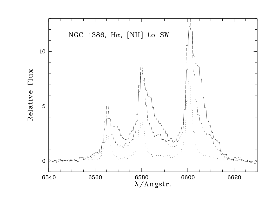
Figure 7: H$\alpha$+[Nii]$\lambda\lambda 6548,6583$ line profiles extracted from 1$\aas@@fstack{\prime\prime}$36 wide spectral scans (of spectrum F080). Continuous line: from region $\cal{B}$ (line maximum); dashed: 1$\aas@@fstack{\prime\prime}$36 southwest; dotted: 2$\aas@@fstack{\prime\prime}$72 southwest.

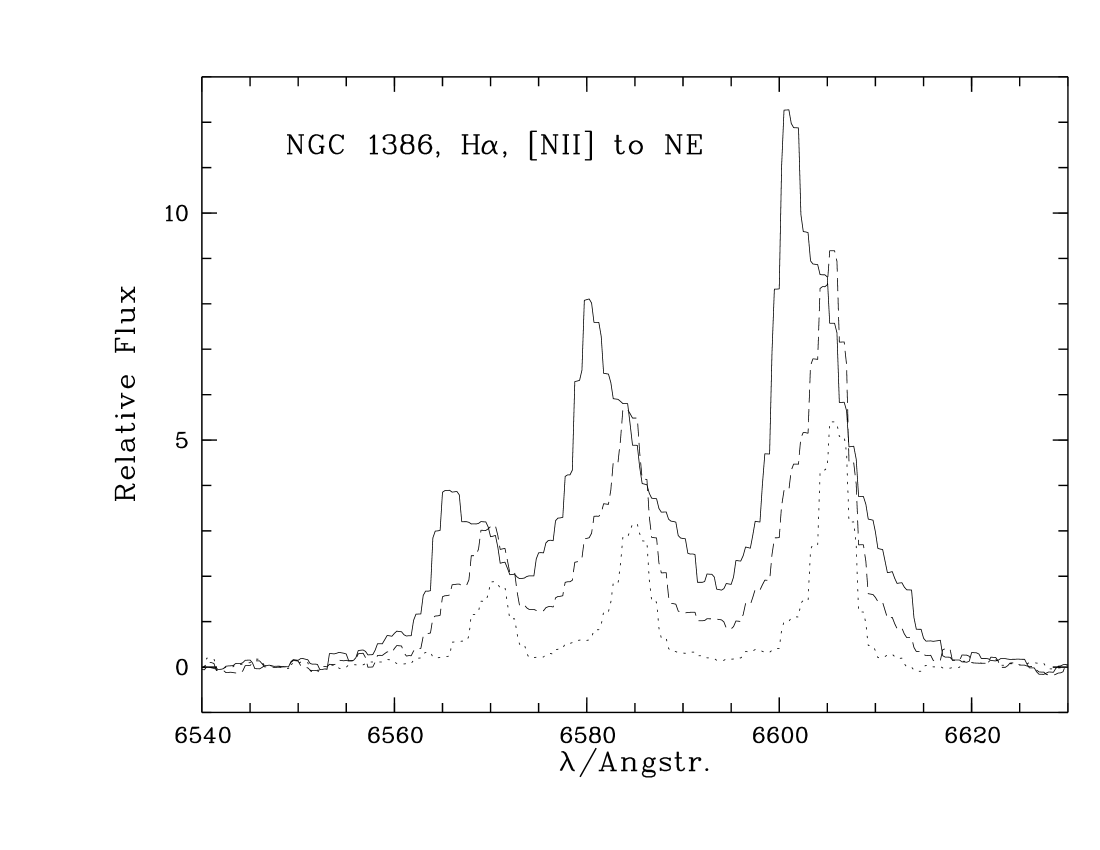
Figure 8: As in Fig. 7, but now towards northeast. Continuous line: from region $\cal{B}$ (line maximum); dashed: 1$\aas@@fstack{\prime\prime}$36 northeast; dotted: 2$\aas@@fstack{\prime\prime}$72 northeast.

In the last subsection we concluded that the spectrum along p.a. 23° arises in an inner gaseous disk that is seen near to edge-on and whose line emitting regions are encompassed by the 2″ wide slit. Hence, we expect line profiles resulting from line-of-sight integrations through the disk.

All profiles have pronounced narrow peaks (called line cores here) with steep flanks. The velocities of the narrow-line cores are given in Table 3. Our spectral resolution is about half of the apparent width of the line core of disk-component $\cal{B}$. The first numerical column in Table 3 gives the velocities of region $\cal{B}$, as measured with different lines. As Figs. 5 to 8 or Table 3 show, the radial velocity of the core of $\cal{B}$ is close to those at 1$\aas@@fstack{\prime\prime}$36 southwest and 2$\aas@@fstack{\prime\prime}$72 southwest, while the regions to the northeast are redshifted. Hence, region $\cal{B}$ is on the ‘blue’ – approaching – side of the rotating disk. In Figs. 6 and 8 we see the core from $\cal{B}$ and the cores from the northeast line profiles together. The radial velocity of the center of the disk (the disk-center velocity) should then be amidst the southwest and northeast cores, at $v_{\rm hel}^{\rm c}=878$ km/s (mean of six spectral lines). This is in agreement with $v_{\rm KC}=877$ km/s determined from folding the outer rotation curve (Sect. 4.2.1).

Table 3: Measured velocities (km/s) of line cores along p.a. 23° in the center of NGC 1386. Uncertainty 15 km/s

Line	At max. (B)	1$\aas@@fstack{\prime\prime}$36 southwest	2$\aas@@fstack{\prime\prime}$72 southwest	1$\aas@@fstack{\prime\prime}$36 northeast	2$\aas@@fstack{\prime\prime}$72 northeast
$[{\rm O}$ iii]$\lambda 4959$	776	757	747	964	983
$[{\rm O}$ iii]$\lambda 5007$	793	762	746	962	984
H$\beta$	777	767	751:	965	965:
$[{\rm O}$ i]$\lambda 6300$	849:	750	741	947	996
H$\alpha$	790	777	770	967	993
$[{\rm N}$ ii]$\lambda 6583$	789	775	768	980	1003
$[{\rm S}$ ii]$\lambda\lambda 6716,6731$	798	776	771	979	1016

Schulz et al. (1995) (their Fig. 4) showed that a rotating edge-on disk with an emissivity law falling with radius will produce asymmetric profiles, with the more extended wing pointing towards smaller absolute values of rotation velocity. However, the wings should not pass the disk-center velocity unless there are strong random motions and/or radiation ‘from the other side’ is scattered in via observational seeing (and guiding inaccuracies), as is shown by an example in Sect. 7.2 of Schulz et al. (1995).

The asymmetric line profiles of component $\cal{B}$ have the extended wing on the side expected for a rotating disk, but their shoulder extends to longer wavelengths than theoretically predicted unless there is strong spatial smearing or an inner high-velocity branch along the same l.o.s. (e.g. central Keplerian rotation). The shoulders even extend beyond the northeast-cores (Figs. 6 and 8). Note that in velocity units the red flank of the core 1$\aas@@fstack{\prime\prime}$36 northeast lies at about the upper limit of the rotation curve in Fig. 4 ($\sim 1050$ km/s) and the blue flank of the core of component $\cal{B}$ (or the core of the component 1$\aas@@fstack{\prime\prime}$36 southwest) lies at the lower limit of the rotation curve ($\sim 700$ km/s). Consequently, the outer red shoulder of profile component $\cal B$ cannot be explained by light from regions of the outer rotation curve, while the sharp transitions to the inner part of the red shoulder (particularly in H$\alpha$ and [Nii] of $\cal B$) and in [Oiii] 1$\aas@@fstack{\prime\prime}$36 southwest suggest that this is emission from the northeast side of the disk. This picture implies that there is nearly no emission seen from the nucleus of the disk at the disk-center velocity (in agreement with the location of KC within the dust lane; see Sect. 4.2.1) as such emission would have smoothed out the transition from the southwest to the northeast component.

Outer wings are found on the blue and red side of component $\cal{B}$ and extend up to 900 km/s symmetrically to the disk-center velocity in [Oiii], but not symmetrically to the core velocity of $\cal{B}$. Wings can also be traced to a slightly lesser extent from the components at 1$\aas@@fstack{\prime\prime}$36 and 2$\aas@@fstack{\prime\prime}$72 distance from $\cal{B}$. In [Nii] outer wings appear to extend to $\sim 700$ km/s.

A possible scattering origin of such wings will be discussed in Sect. 5.1.2. Since the kinematical center is obscured by the dust lane, an explanation by fast Keplerian motion close to the disk center is unlikely.

Spectrum F023 taken along p.a. 90° (along which FWM2000 detected two emission-line plumes) shows emission over $\pm 2\arcsec$  with a slightly declining velocity gradient from east to west ($\sim 5$ km/s/″). The near-north-south orientation of the disk explains why a notable east-west gradient in the l.o.s. projections of rotational motions is unexpected. Its near-edge-on orientation makes the detection of minor-axis outflow difficult. The gradient could be due to outflow along the plumes if the disk is slightly tilted from edge-on. The extended red wing in H$\alpha$, [Nii] and [Sii] (seen in the F080 spectrum of component B (continuous line) in Figs. 7 and 8) is confirmed by F023.

4.2.3 Line ratios

Albeit of the primarily kinematic nature of the present study, a few relative intensities of the major diagnostic lines are to be noticed in order to identify the nature of the emission-line region in question. Weaver et al. (1991) noticed a wealth of varying emission-line ratios from the typical Sy-2 high-excitation ratios to extranuclear LINER-like ratios. Even in the few strips that our spectra cover, drastic line-ratio changes are seen. Along the p.a. (23°, 23°+180°) slit, [Nii]$\lambda 6583$/H$\alpha$, [Sii]($\lambda 6716$+$\lambda 6731$)/H$\alpha$ and [Oi]$\lambda 6300$/H$\alpha$ increase from 1.5, 0.68 and 0.13 at the brightness maximum ($\cal B$) to 2.5, 1.10, 0.23, respectively, at 4″ southwest. To the northeast there is only a moderate (10%) increase towards 3″ northeast in [Nii] and [Sii], only [Oi] rises to 0.2.

[Oiii]/H$\beta$ is 13 at $\cal B$, but rises to 21 at 1$\aas@@fstack{\prime\prime}$36 southwest, and 17 at 1$\aas@@fstack{\prime\prime}$36 northeast. [Sii]$\lambda 6716$/[Sii]$\lambda 6731$ is 1.0 at $\cal B$ (indicating $n_{e}=7\,10^{2}$ cm^-3) and 1$\aas@@fstack{\prime\prime}$36 southwest, but rises to 1.2 for the next 3″ on either side (indicating an average $n_{e}=2.5\,10^{2}$ cm^-3).

A faint spectrum along p.a. 90° (F026), with the slit set 2″ north of $\cal B$, shows essentially constant values $\sim 1$ and $\sim 0.8$ ($n_{e}\approx 10^{3}$ cm^-3) for [Nii]$\lambda 6583$/H$\alpha$ and [Sii]$\lambda 6716$/[Sii]$\lambda 6731$ over about 10″, respectively.

4.3 The LINER NGC 1052

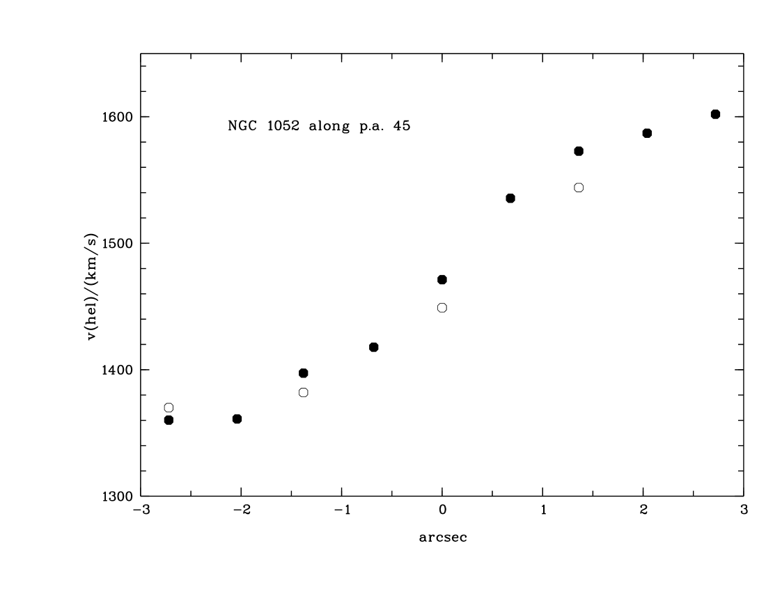
Figure 9: Heliocentric velocities/(km/s) along p.a. 45°in the center of NGC 1052 (northeast to the left). The filled octagons show the mean positions of the line peaks of H$\alpha$ and [Nii]$\lambda 6583$ as measured in the raw spectrum. The open octagons display the mean values of single-component Lorentzian fits given in Table 4.

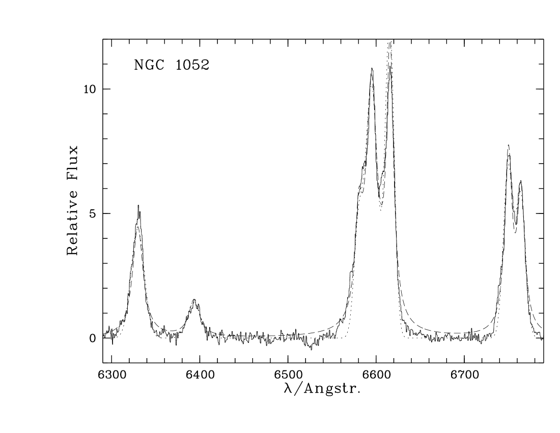
Figure 10: Red spectrum (including [Oi]$\lambda\lambda 6300,6363$, H$\alpha$+[Nii]$\lambda\lambda 6548,6583$, and [Sii]$\lambda\lambda 6716,6731$) from the brightness maximum ($1\aas@@fstack{\prime\prime}36\times 2\arcsec$) of NGC 1052 with the slit aligned along p.a.45°. Fits with single Lorentzians (dashed) or Gaussians (dotted) are insufficient. Positions and line widths from the fits with Lorentzians are given in Table 4 (column headed by 0).

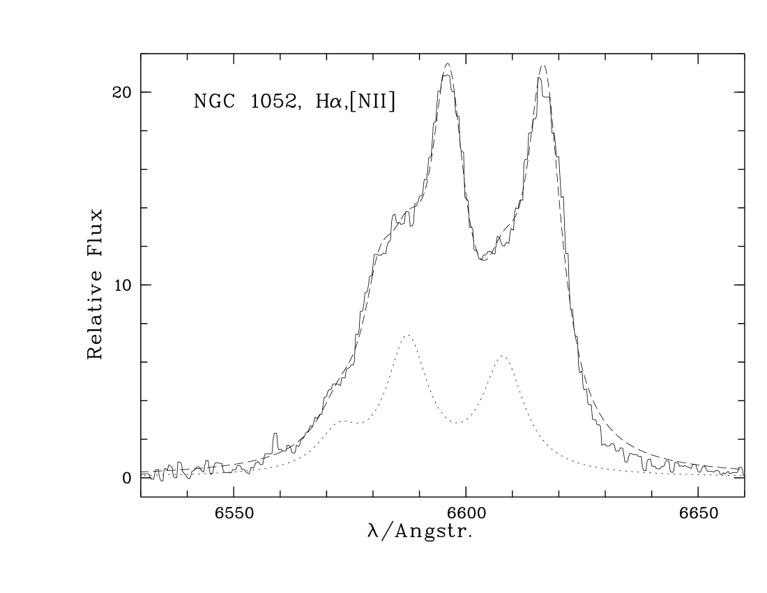
Figure 11: Two narrow-line systems $\cal{A}$ and $\cal{B}$, each characterized by three Lorentzian functions with fixed line width and position in velocity space (the intensity ratio of $\lambda 6583$ to $\lambda 6548$ is fixed to 3 to 1), are sufficient to fit the observed H$\alpha$+[Nii]$\lambda\lambda 6548,6583$ blend from the region with maximum emission (continuous line shown above) and till 2″ northeast. H$\alpha$+[Nii] from system $\cal{B}$ (dotted) and the ‘fitting’ sum $\cal{A}+\cal{B}$ (dashed) are shown. While $\cal{B}$ is blueshifted and indicates outflow, $\cal{A}$ is consistent to arise in a rotating disk.

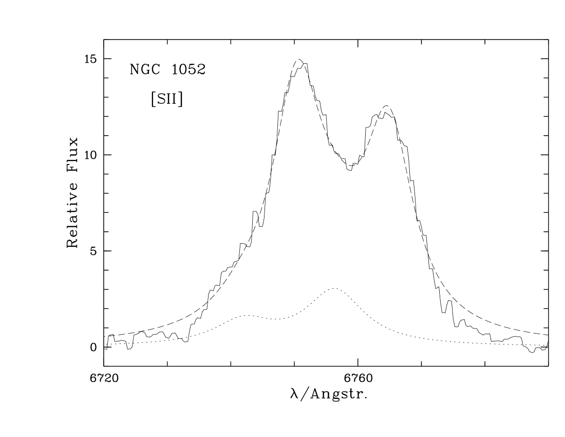
Figure 12: As in Fig. 11, but now for [Sii]$\lambda\lambda 6716,6731$. Component $\cal{B}$ is additionally constrained to be in the high-density limit ($n_{e}\gg 10^{3}$ cm^-3).

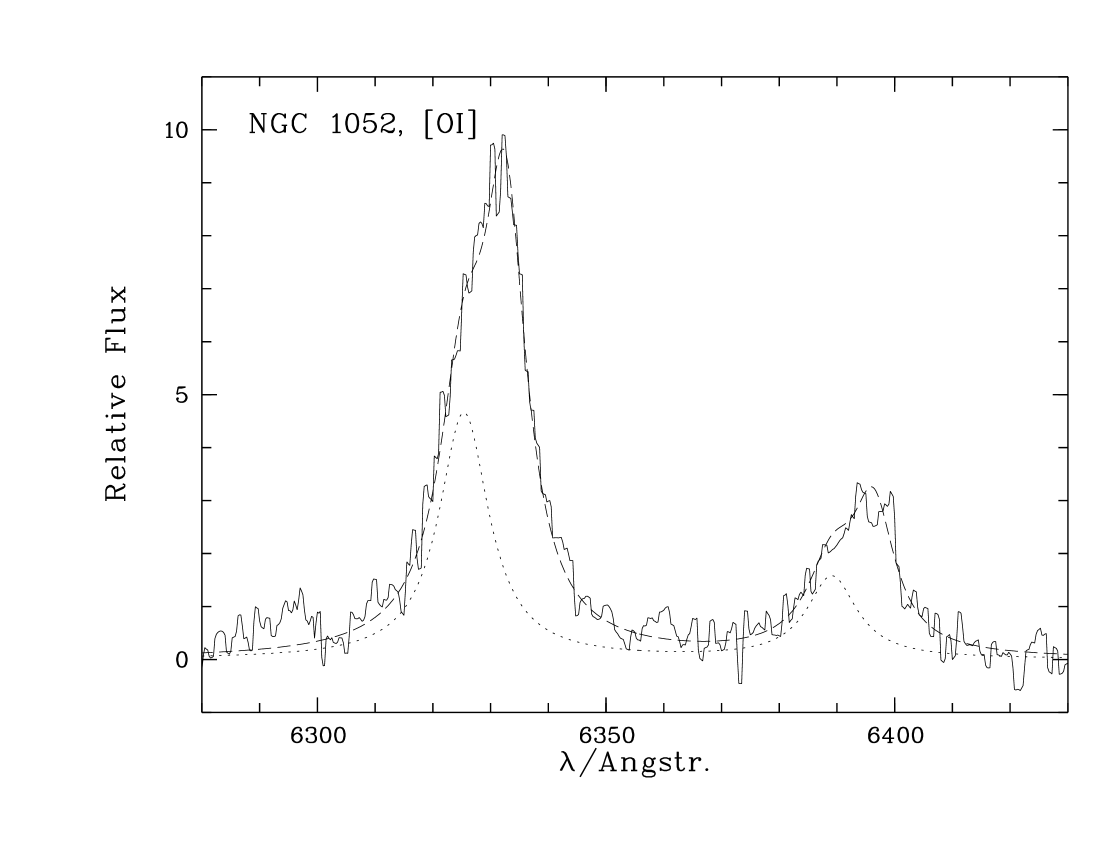
Figure 13: As in Fig. 11, but now for [Oi]$\lambda\lambda 6300,6363$.

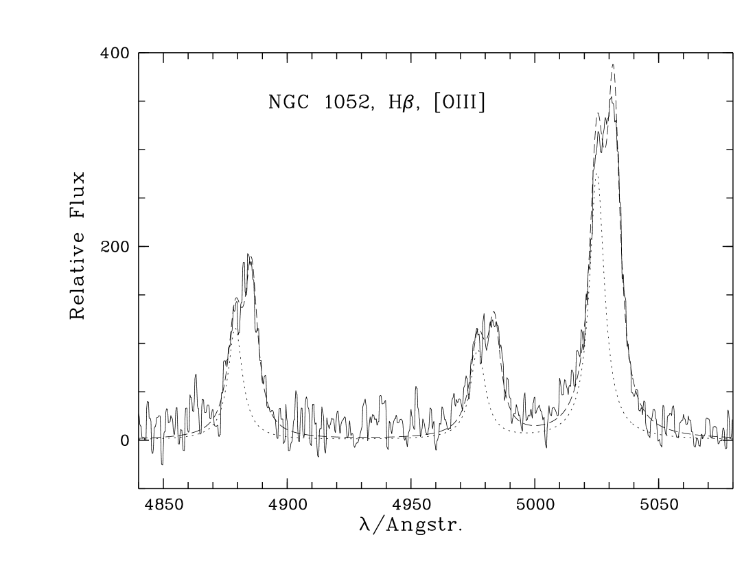
Figure 14: As in Fig. 11, but now for H$\beta$ and [Oiii]$\lambda\lambda 4959,5007$.

4.3.1 Fitting line profiles with single components

Davies & Illingworth (1986) gave p.a. 49° as the approximate position angle of the major axis of the nuclear gaseous disk in NGC 1052. For deprojecting the observed velocities we assume that spectra F078 and F107 (slit along p.a. $45^{\circ}$) were taken along the major axis.

Fig. 9 shows two major-axis velocity curves; one shows the positions of the peaks of H$\alpha$ and [Nii]$\lambda 6583$ in the raw spectra from 0$\aas@@fstack{\prime\prime}$68 row extractions. The other curve corresponds to template-corrected spectra binned to 1$\aas@@fstack{\prime\prime}$36 wide spectral extractions and displays the mean values of single-component Lorentzian fits (see Table 4) of the lines H$\alpha$, [Nii]$\lambda\lambda 6548,6583$, and [Sii]$\lambda\lambda 6716,6731$ from the disk (see Appendix B regarding the fitting procedures with Gaussians and Lorentzians as basic functions). Beyond the steep central gradient the curves flatten out. They are not symmetric relative to the zero point, which is located at the brightness maximum.

Davies & Illingworth (1986) identified a nuclear ionized disk that emits most of the emission-line spectrum. For subsequent mass estimates an inclination of the disk $i=60\degr$ is assumed as derived in the following subsection (note that Bertola et al. (1993) obtained $i=53\degr$ from the data of Davies & Illingworth; this value would increase the mass estimates given below by 18%).

The central velocity gradient (between maximum and two adjacent pixels) of 85 km/s/″  translates formally into 59.2 km/s/(50pc), yielding a Keplerian mass of $4.1\,10^{7}$ M_⊙ inside a radius of 50 pc, which corresponds to the inner, just resolved core with 1$\aas@@fstack{\prime\prime}$2 diameter.

The processed data (Table 4) have 1$\aas@@fstack{\prime\prime}$36 resolution and lead to a gradient of 110 km/s per 2″ radius (measured at a velocity of 1478 km/s), which translates into $6.3\,10^{8}$ M_⊙ inside a radius of 166 pc.

Albeit crude, these mass estimates imply that NGC 1052 has a core of relatively small mass. In order to judge the reliability of these numbers a closer look on the fits is needed.

The data given in Table 4 were obtained by the Lorentzian fits of [Oi]$\lambda\lambda 6300,6363$, H$\alpha$, [Nii]$\lambda\lambda 6548,6583$, and [Sii]$\lambda\lambda 6716,6731$ shown in Fig. 10. Although fitting the major part of the profiles these fits are unsatisfactory in several respects.

Firstly, measured outer line wings appear too weak or too strong as compared to Lorentzian or Gaussian fits, respectively. In itself, this might not be taken as serious because it could simply reflect the deficiency of these functions in comparison to the typical core-wing structure of narrow-line profiles.

Secondly, the final summed fit lies systematically below the bridges connecting [Nii]$\lambda 6548$ and H$\alpha$ or [Nii]$\lambda 6583$ and H$\alpha$, and connecting the [Sii] lines. It also lies below the blue wing of [Nii]$\lambda 6548$. This holds irrespective of the type of profile function.

Thirdly, although no conspicuous asymmetry is seen in [Oi], in this case the fit function turns out to be blueshifted by $\sim 100$ km/s and appears 80% wider with respect to other forbidden lines. Also, sometimes H$\alpha$ requires considerably larger widths than [Nii] although its position is not significantly shifted (Table 4).

These findings indicate that the line profiles are complex and that a one component model is not sufficient for an appropriate simulation. In the next subsection we therefore decompose the line profiles in a more detailed manner.

Table 4: This table gives heliocentric velocities and (after the $|$) values of $w$=FWHM (in km/s) derived by single-component Lorentzian fits in template-corrected 1$\aas@@fstack{\prime\prime}$36 wide spectral extractions along p.a. 45° of NGC 1052. For [Oi] and [Nii] the doublet ratios 3:1 and the requirement of same widths (as in [Sii]) additionally constrain the fits. The column labeled ‘0’ refers to the 1$\aas@@fstack{\prime\prime}$36 wide spectral scan at maximum emission. Last row: mean values of the lines H$\alpha$, [Nii]$\lambda\lambda 6548,6583$, and [Sii]$\lambda\lambda 6716,6731$ (open octagons in Fig. 9).

Line	5$\aas@@fstack{\prime\prime}$44 NE	4$\aas@@fstack{\prime\prime}$08 NE	2$\aas@@fstack{\prime\prime}$72 NE)	1$\aas@@fstack{\prime\prime}$36 NE	0	1$\aas@@fstack{\prime\prime}$36 SW	2$\aas@@fstack{\prime\prime}$72 SW	4$\aas@@fstack{\prime\prime}$08 SW	5$\aas@@fstack{\prime\prime}$44 SW
H$\alpha$	$1330|161$	$1369|137$	$1369|226$	$1376|492$	$1430|706$	$1531|545$	$1594|270$	$1615|196$	$1614|172$
$[{\rm N}$ ii]	$1363|168$	$1381|128$	$1366|205$	$1380|316$	$1446|435$	$1552|383$	$1607|299$	$1631|229$	$1629|201$
$[{\rm S}$ ii]	$1342|178$	$1374|156$	$1374|229$	$1391|365$	$1471|454$	$1550|393$	$1605|264$	$1645|208$	$1621|200$
$[{\rm O}$ i]$\lambda 6300$	—	$1361|360$	$1325|401$	$1330|647$	$1373|711$	$1469|709$	$1622|331$	—	—
mean	$1345|169$	$1375|140$	$1370|220$	$1382|391$	$1449|532$	$1544|440$	$1602|278$	$1630|211$	$1621|191$

4.3.2 Decomposition of the line profiles

In view of the problems encountered with single-component fits, a significant improvement may be obtained by a mixture of two line systems, conveniently denoted as $\cal A$ and $\cal B$, with system $\cal B$ blueshifted with respect to $\cal A$.

In Fig. 11 a fit to H$\alpha$ + [Nii] from the ‘central’ (center defined by maximum emission) $2\arcsec\times 0\aas@@fstack{\prime\prime}68$ (slit width $\times$ width of CCD extraction row) is shown along p.a. 45^∘. The line blend can indeed be successfully decomposed into two narrow-line H$\alpha$ + [Nii] systems. However, such a fit of a smeared out blend of lines can only be found by the software if guided by strong constraints, which we are now going to justify.

In Table 5 final results for the FWHMs, velocities and line ratios of systems $\cal A$ and $\cal B$ are given. The data are restricted to the spatial regime between 2″ northeast and 0$\aas@@fstack{\prime\prime}$68 southwest for which component $\cal B$ can be unambiguously recognized.

Table 5: Line widths $w$=FWHM, heliocentric velocities and line ratios measured for the rotational component $\cal{A}$ and the outflow component $\cal{B}$ (separated by a $|$) along p.a. 45° from 0$\aas@@fstack{\prime\prime}$68 southwest to 2$\aas@@fstack{\prime\prime}$04 northeast in NGC 1052.

	2$\aas@@fstack{\prime\prime}$04 NE	1$\aas@@fstack{\prime\prime}$36 NE	0$\aas@@fstack{\prime\prime}$68 NE	0	0$\aas@@fstack{\prime\prime}$68 SW
$w({\cal A})|w({\cal B})$	$268|208$	$296|366$	$378|435$	$420|498$	$340|565$
Line
H$\beta$, [Oiii]	$1354|931$	$1407|1059$	$1468|1064$	$1496|1081$	$1629|1342$
H$\alpha$, [Nii]	$1371|998$	$1414|1043$	$1449|1066$	$1505|1096$	$1567|1249$
$[{\rm S}$ ii]	$1369|$ —	$1414|1109$	$1448|1066$	$1498|1154$	$1559|1353$
$[{\rm O}$ i]	$1355|992$	$1397|1016$	$1484|1141$	$1506|1165$	$1575|1256$
mean	$1364|980$	$1409|1054$	$1460|1081$	$1502|1116$	$1579|1290$
mean$-1502$	$-138|-522$	$-93|-448$	$-42|-421$	$0|-386$	$77|-212$
$I(\lambda 5007)/I$(H$\beta$)	$1.97|1.94$	$1.74|2.69$	$2.03|2.43$	$1.71|2.82$	$2.03|2.15$
$I(\lambda 6583)/I$(H$\alpha$)	$1.16|1.37$	$1.12|1.32$	$1.05|1.09$	$1.09|0.86$	$1.23|0.89$
$I$([Sii]${}_{\rm tot}/I$(H$\alpha$)	$1.29|$ —	$1.13|0.90$	$1.18|0.84$	$1.36|0.62$	$1.58|0.91$
$I(\lambda 6300)/I$(H$\alpha$)	$0.48|1.79$	$0.58|0.57$	$0.48|0.87$	$0.45|0.66$	$0.39|0.59$
$I(\lambda 6716)/I(\lambda 6731)$($\cal{A}$)	1.40	1.15	1.04	1.17

The H$\alpha$+[Nii] blend has been fit by assuming that all three lines in each system are constrained to have the same radial velocity and line width $w$ (=FWHM; see Appendix B) while the intensities of H$\alpha$ and [Nii] are left free (the 3:1-[Nii] ratio is fixed; see Appendix B). Each of the two systems is fixed by four parameters (same position and same width in velocity space, height of H$\alpha$ and height of [Nii]$\lambda 6548$). Thus, only eight parameters are fit for six line profiles which would be determined by eighteen parameters in total if each single profile were free of constraints.

A slight shoulder on the blue wing of [Sii]$\lambda 6716$ requires the presence of the blueshifted component in [Sii] as well. An example for a fit of the [Sii] system employing analogous precepts as for H$\alpha$ + [Nii] (adopting $w(\cal A)$ and $w(\cal B)$ from the H$\alpha$ + [Nii] fit of each region) is shown in Fig. 12. Five out of twelve parameters were fit (two velocities, for systems $\cal{A}$ and $\cal{B}$, two amplitudes for system $\cal{A}$ and one amplitude for system $\cal{B}$, where the [Sii] intensity ratio was fixed to $I(6731)/I(6716)=2.3$, which is the saturation limit for electron densities $n_{e}\gg 10^{3}$ cm^-3).

A large electron density of $\cal{B}$ has been chosen to increase the contribution of [Oi]$\lambda\lambda 6300,6363$ relative to [Sii]$\lambda\lambda 6716,6731$. The critical density of the upper [Oi] levels, $1.7\,10^{6}$ cm^-3, is three orders of magnitude above that for [Sii]. A high electron density is indicated by the single-component fits which yield large relative strengths of [Oi] in the diagnostic diagrams of Veilleux & Osterbrock (1987; hereafter VO) and larger line widths than those of [Sii] and [Nii] (Table 4). The trend that [Oi] can be boosted mainly by density is shown in Komossa & Schulz (1997; their Fig. 4, upper panel). Even though a distinct blue peak or a clear shoulder is missing in [Oi]$\lambda 6300$ (Fig. 13), the two-component fit with Lorentzian functions is satisfactory and explains the greater width of the [Oi] profiles by a relatively strong $\cal{B}$ contribution.

Due to the likewise high critical density of $7\,10^{5}$ cm^-3 of the ${}^{1}{\rm D}_{2}$ upper term of [Oiii]$\lambda\lambda 4959,5007$, these lines may be density-boosted in high-ionization zones. Consequently component $\cal B$ might be conspicuous in these lines as well which is indeed verified by a significant blue shoulder of the profiles (Fig. 14). The [Oi] and [Oiii] spectra were consequently fit in the same way as the [Sii] lines; making use of 3:1-line ratios in each of the oxygen doublets, however, four free parameters out of a total of twelve were sufficient, one amplitude and one velocity for each of the two systems, $\cal{A}$ and $\cal{B}$, respectively.

The row ‘mean’ in Table 5 gives the average velocities over the four line groups (H$\beta$+[Oiii], [Oi], [Sii], H$\alpha$+[Nii], the latter is weighted twice) for velocity systems $\cal{A}$ and $\cal{B}$. The line velocities for system $\cal{A}$ given in Table 5 are consistent with arising in a rotating circumnuclear disk (as suggested by Davies & Illingworth 1986). The differences relative to 1502 km/s (next row) exhibit a nearly linear gradient to the northeast of 57 km/s per 0$\aas@@fstack{\prime\prime}$68 step (=56.37 pc) or 51 km/s at a formal radius of 50 pc from the kinematical center (which appears to be slightly shifted from the location of maximum emission). This would lead to a Keplerian mass estimate of $3\,10^{7}$ M_⊙ inside 50 pc if the disk were edge-on, or $4\,10^{7}$ M_⊙ for $i=60\degr$ as given below. The latter value is in agreement with the single component fits given in Sect. 4.3.1 because the blue component $\cal{B}$ hardly effects the overall fits (except for [Oi] which was not considered in the mean values of Table 4).

Two slightly poorer spectra along p.a. 90°(F020 and F056) were decomposed in a similar way (with outflow fixed by 400 km/s). From these a component–$\cal{A}$ gradient of 15 km/s per 0$\aas@@fstack{\prime\prime}$68 was found. With p.a. (major axis) = 45° we can adjust the velocity deprojection factor of Eq. 3 so that along both slit directions the rotational velocities in the disk agree. This procedure leads to an inclination angle $i=60\degr\pm 5\degr$.

The blueshifted system $\cal{B}$ is most likely explained by the presence of outflowing gas. At various p.a. blueshifted structure in the wings of [Oiii] were earlier described by Davies & Illingworth (1986). Although they had not attempted a quantitative numerical decomposition of their line profiles, their insightful discussion led to the detection of widespread outflow on the eastern side of the nucleus.

The spatial covering of the present data is insufficient for clues about specific outflow geometries of component $\cal{B}$. Also, prior to deeper interpretation the degree of uniqueness of the fit-procedure has to be discussed. To this end, we had also attempted fits with other constraints, e.g. fixing the blueshift of $\cal{B}$ (at 400 km/s relative to $\cal{A}$) rather than fixing the line width. The kinematics of the rotational component $\cal{A}$ was hardly altered suggesting that common velocities and linewidths in lines from different ions are a robust feature for a bulk component.

Despite general agreement, to the northeast Table 5 shows differences in the outflow velocities of up to $\sim 70$ km/s. Such differences are within the accuracy of the fitting procedure that employs a simple basic function. Note that most differences are significantly below the component widths and the spectral resolution. The worst discrepancies are at 0$\aas@@fstack{\prime\prime}$68 southwest, but here the outflow component starts to vanish.

Row ‘mean–1502’ in Table 5 gives the l.o.s. components of the outflow velocity relative to the emissivity maximum, identified at 1502 km/s. On the northeastern side it is blueshifted by $\sim(450\pm 70)$ km/s; at 0$\aas@@fstack{\prime\prime}$68 southwest less consistent fits yield a blueshift of $\sim 200$ km/s.

With a disk inclination angle of 60° the northeast outflow velocity would be $\sim 900$ km/s relative to the emissivity maximum if it were directed along the minor axis. However, a detailed deprojection has to await more complete data.

4.4 The Seyfert Mrk 1210

4.4.1 The WR-feature

The three spectra extracted from F116 (Table 1) with $2\arcsec$ wide bins from the central $6\arcsec$ (diameter) exhibit HeII$\lambda 4686$ with an observed intensity of 25% of H$\beta$.

Concentrated in the central 2″ we detect a Wolf-Rayet feature around $\lambda 4686$ (for Mrk 1210 first shown in Storchi-Bergmann et al. 1998).

Considering individual features, we note that [Feiii]$\lambda 4658.10$ is clearly present, [Ariv]$\lambda 4740.34$ is present outside the innermost $2\arcsec$, while [Ariv]$\lambda 4711.34$ and [Neiv]$\lambda 4724.15$ are possibly present, but cannot be clearly discerned at our signal-to-noise level.

The WR-feature is an unambiguous sign for the presence of a starburst which appears to arise cospatial with the NLR or in a region roughly seen in projection to the inner kiloparsec in which the bright part of the AGN NLR is situated.

4.4.2 Analysis based on single narrow-line component

Firstly, peak positions of the strongest lines were measured. The derived nuclear velocity curve along p.a. 90°  yields a small velocity gradient (Fig. 15). The gradient is flattened because of seeing and guiding inaccuracies of $\sim 2\arcsec$. A deconvolution is not warranted because of the lack of an appropriate point-spread function.

Locating the kinematical center KC midway within the slope yields a measured difference to the brightness maximum BM of 1$\aas@@fstack{\prime\prime}$5. In the weaker blue spectrum (F116) the slope plus three extraction rows westwards can be measured in [Oiii]. Here the difference between KC and the [Oiii] BM amounts to two rows or 1$\aas@@fstack{\prime\prime}$3. Due to the spatial smearing the real difference is likely $\sim 1\arcsec$ or slightly less.

From velocities measured in the weak spectra (F085, F087), which were obtained offset from the brightness center by 2″ (slit along p.a. 90°) we estimate a p.a. of the kinematical major axis of $110\degr\pm 20\degr$. The uncertainty of the p.a. is due to the faintness of the extranuclear lines.

From the observed slight velocity variations one cannot safely distinguish between bipolar outflow and rotation. We tend to regard it as a reflex from the rotating nuclear kpc-spiral disk seen in a snapshot-HST-image (Malkan et al. 1998). However, neither from the kinematical data nor from the printed HST image a meaningful value of inclination can be derived, so that no reliable mass estimate can be given.

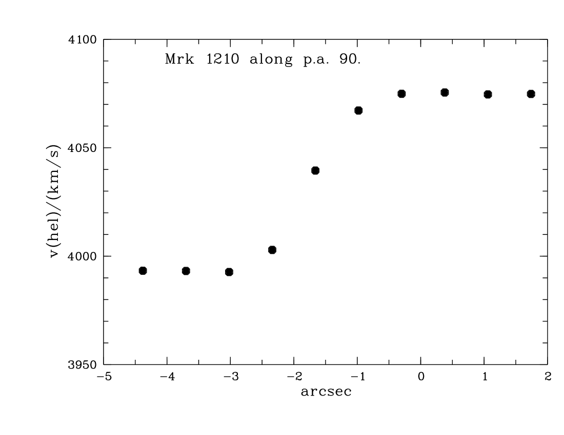
Figure 15: Velocity curve (heliocentric) of Mrk 1210 based on the mean of the peak positions of H$\alpha$ and [Nii]$\lambda 6583$ in the raw spectrum F066 along p.a. 90°(east to the left). The brightness maximum is at the zero position. The curve is smoothed by spatial smearing ($>2\arcsec$).

Table 6: Heliocentric velocities and line widths (FWHM) (separated by $|$ ) in km/s along p.a.  90° through the nucleus of Mrk 1210 as derived from single-component Lorentzian fits. The zero position is that of the interpolated brightness maximum (symmetry center of brightness).

Position	H$\beta$	[Oiii]	[Oi]	H$\alpha_{\rm broad}$	H$\alpha_{\rm narrow}$	[Nii]	[Sii]
3$\aas@@fstack{\prime\prime}$02 E			$3992|809$	$3999|2268:$	$3999|116$	$3998|137$	$3999|148$
2$\aas@@fstack{\prime\prime}$34 E	$4008|329$	$4001|471$	$4076|715$	$4004|1893$	$4004|188$	$4019|213$	$4017|177$
1$\aas@@fstack{\prime\prime}$66 E	$4021|450$	$4034|507$	$4104|605$	$4048|1759$	$4048|313$	$4052|296$	$4053|256$
0$\aas@@fstack{\prime\prime}$98 E	$4056|557$	$4054|495$	$4127|617$	$4076|1733$	$4076|331$	$4081|287$	$4072|274$
0$\aas@@fstack{\prime\prime}$30 E	$4066|595$	$4063|494$	$4133|607$	$4088|1707$	$4088|351$	$4092|319$	$4081|276$
0$\aas@@fstack{\prime\prime}$38 W	$4043|486$	$4051|572$	$4135|587$	$4089|1703$	$4089|392$	$4095|328$	$4083|271$
1$\aas@@fstack{\prime\prime}$06 W	$4055|474$	$4058|505$	$4126|631$	$4084|1684$	$4084|396$	$4091|319$	$4084|275$
1$\aas@@fstack{\prime\prime}$74 W	$4017|421$	$4042|478$	$4097|640$	$4078|2429$	$4078|267$	$4074|212$	$4088|227$
2$\aas@@fstack{\prime\prime}$42 W				$4092|5129:$	$4092|137$	$4076|144$	$4094|166$

Leaving aside the global kinematics, various trial fits of the strongest line profiles (observed to the west of the location of the velocity gradient) were undertaken which led to reasonably successful single-component fits. For justification of the results given in Table 6 and, in particular for an alternative decomposition of the profiles described in the next subsection, some details of the procedures employed are to be explained.

Firstly, it was attempted to fit the apparent three-line blends H$\alpha$+[Nii] by either a sum of three Gaussians or three Lorentzian functions only constrained by the 3-to-1 intensity ratio (and same width) of [Nii]. These fits badly failed, although the Lorentzians yielded smaller but yet unacceptably large residuals. The ratio of the measured peaks of $\lambda 6583$ and $\lambda 6548$ in the blend is only 1.8 to 1 instead of the expected 3-to-1 ratio. This indicates that the flux from an additional component is stronger beneath $\lambda 6548$ than below $\lambda 6583$, which can be relatively easily achieved by the contribution of a broad H$\alpha$ component in addition to narrow H$\alpha$. The wide Lorentz wings of a single H$\alpha$ component (allowed to be broader than the [Nii] lines) cannot lift $\lambda 6548$ sufficiently.

All trial fits with an additional broad component assume it to be at the same central wavelength as the narrow H$\alpha$ feature. One broad component, either Gaussian or Lorentzian, does not lead to a satisfactory fit if three narrow Gaussians are added, due to their typical ‘lack of wings’. Solely equipped with Gaussians, one would need many more than these four components for an acceptable fit.

Three narrow and one broad Lorentzian function produce too much flux in the outskirts of the blend suggesting that the real underlying broad component does not have extended wings. Indeed, the best four-line fits were obtained with three narrow Lorentzians and one broad Gaussian concentric with the narrow Lorentzian of H$\alpha$ (as shown in Fig. 16).

Qualitatively, the presence of a broad H$\alpha$ component is not unexpected in view of the polarized (degree of polarization $\sim 1\%$) broad H$\alpha$ found in Mrk 1210 (Tran 1995). However, the faint polarized flux should not give such a strong signal in total flux.

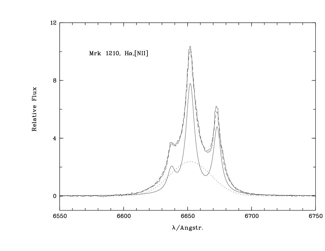
Figure 16: H$\alpha$+[Nii]$\lambda\lambda 6548,6583$ from 0$\aas@@fstack{\prime\prime}$68 east of the region where lines are at maximum. The total fit (dashed line) consisting of a sum of three Lorentzians (continuous line) for narrow H$\alpha$ and [Nii] (the [Nii] lines are constrained by the 3:1-ratio and the same width) plus a broad Gaussian (dotted) concentric with the narrow Lorentzian that fits the core of H$\alpha$.

The good single-component fits of [Nii] suggest to fit the other strong forbidden-systems by single Lorentzian functions as well (with the joint constraints as given in Appendix B). The resulting velocities and line widths from these single-component fits are given in Table 6. In general, these simple fits reproduce the gross structures relatively well and may be considered as a success for the Lorentzian functions because single Gaussians fail to represent the wings of all major lines.

Even H$\beta$ can be represented by a single Lorentzian, somewhat wider than the above fit of narrow H$\alpha$ and much narrower than broad H$\alpha$ (Fig. 17, Table 6). This means that with the chosen fitting procedure the profiles of H$\alpha$ and H$\beta$ do not agree. The broad+narrow component decomposition of H$\alpha$ cannot be transferred to H$\beta$ by allowing for different values of extinction for the components.

A close look unveils marked imperfections in the forbidden-line fits as well. E.g., the [Oiii] lines are asymmetric to the blue (Fig. 17), in the [Sii] blend a residual excess remains in the red wing (Fig. 18). [Oi] shows structure and is redshifted relative to the other lines (Fig. 19, Table 6). In addition, the [Oiii] and [Oi] lines ($w\sim 600$ km/s) are significantly wider than the [Nii] and [Sii] lines ($w\sim 300$ km/s). Altogether, a more sophisticated decomposition is required which will be proposed in the next subsection.

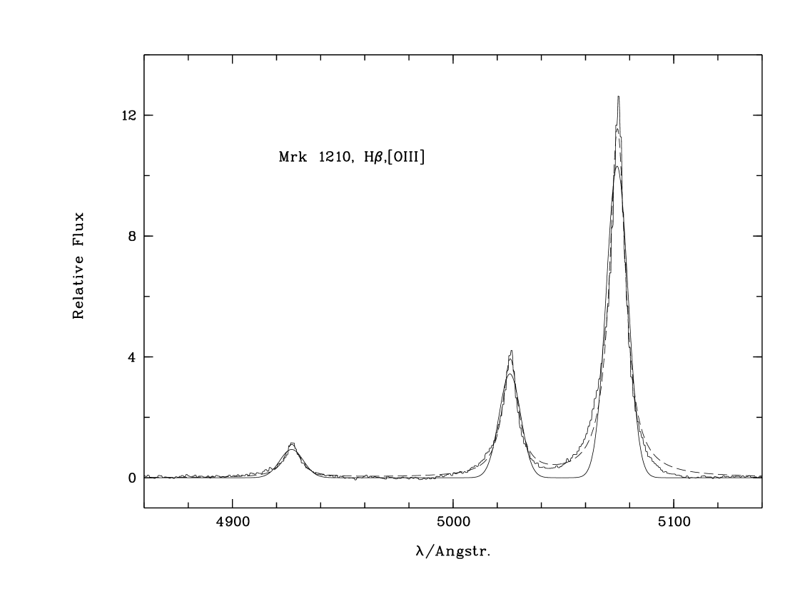
Figure 17: As in Fig. 16, but for H$\beta$ and [Oiii]$\lambda\lambda 4959,5007$ as fit by single Lorentzian functions (dashed). The [Oiii] lines are constrained by the 3:1-ratio and equal width. Obviously they have a blueward wing asymmetry. The smooth continuous line shows the analogous, but much inferior fit with Gaussians.

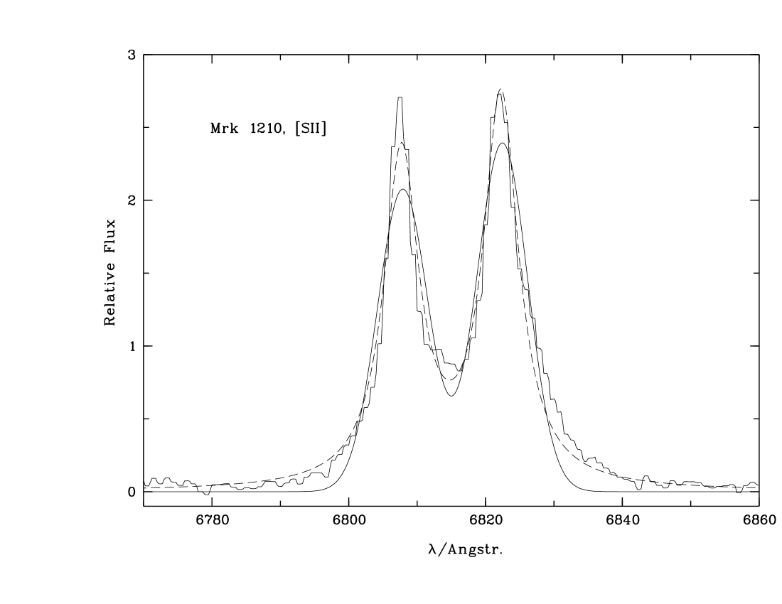
Figure 18: [Sii]$\lambda\lambda 6716,6731$ from the same region as in Fig. 16 as fit by two Lorentzians (dashed) with same width and position in velocity space. A fit with two Gaussians and otherwise same presumptions is displayed by the smooth continuous line. Athough not perfect, single Lorentzians appear to be better suited as basic fit functions than single Gaussians.

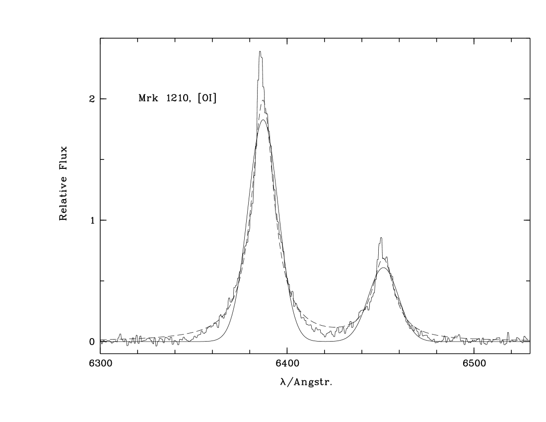
Figure 19: As in Fig. 16, but for [Oi]$\lambda\lambda 6300,6363$ as fit by two Lorentzians (dashed) with same width and position in velocity space. Smooth continuous line: The analogous trial fit with Gaussians.

Table 7: Relative intensity ratios of components $\cal{M}$, $\cal{R}$ and $\cal{B}$ as defined by corresponding velocity-width parameters $(v,w)(\cal{M})$ = (4064, 208), $(v,w)(\cal{R})$ = (4304, 350) and $(v,w)(\cal{B})$ = (3895, 727) (in km/s). The intensity of the line-core component $\cal{M}$ is set to unity. (1) and (2) correspond to alternative fits of the H$\alpha$+[Nii] blend (Figs. 24 and 25), respectively.

Line	$\cal{R}$(1)	$\cal{B}$(1)	$\cal{R}$(2)	$\cal{B}$(2)
$[{\rm O}$i]	1.65	2.05
$[{\rm S}$ ii]$\lambda 6716$	0.18	0.07
$[{\rm S}$ ii]$\lambda 6731$	0.41	0.17
$[{\rm N}$ ii]	0.42	1.74	0.29	0.90
H$\alpha$	0.42	1.73	0.76	1.71
H$\beta$	0.65	2.24
$[{\rm O}$ iii]	0.44	1.97

4.4.3 The decomposition of the line profiles

Table 6 shows that the velocities of the single-component fits for emission from between 0$\aas@@fstack{\prime\prime}$98 east and 1$\aas@@fstack{\prime\prime}$06 west agree within 10 km/s so that we combined the lines to represent the total emission from the $\pm 1\arcsec$ of the brightness maximum. This gives practically no difference to fits of single extraction-rows, but reduces the noise and is more appropriate in view of the width of the spatial point-spread function of $\sim 2\arcsec$.

The red wings seen in the [Sii] and [Oi] profiles and the large widths of [Oi], H$\beta$ and [Oiii] suggest the presence of different kinematical components. However, the H$\beta$ and [Oiii] profiles and the H$\alpha$+[Nii] blend are lacking clear substructure for providing anchoring features to constrain different components. At first, we therefore looked for guidance by visible structures in other lines and attempted to apply the resulting components with the same widths and positions to the smoother profiles.

Fig. 20 shows a three-component Lorentzian fit to [Sii]. $\cal{M}$ (not displayed) is the ‘main’ component determined by the peaks of the profiles, which therefore has the closest relation to the velocity curve in Fig. 15. The red-shifted component $\cal{R}$ has been invoked to fit a residual shoulder on the red side and the inter-line regime. The relative strength of the two [Sii] lines of $\cal{M}$ is a free parameter. As in the case of NGC 1052, we assume that the particular strength of [Oi] is partially due to the second component (here: $\cal{R}$) with $n\gg 10^{3}$ cm^-3, which fixes its intensity ratio [Sii]$\lambda 6731$/[Sii]$\lambda 6716=2.3$. The components are $\cal{M}$ (‘main’) and $\cal{R}$ (‘red’) defined by ($v$=heliocentric velocity, $w$=FWHM), both measured in km/s. The fit gives $(v,w)(\cal{M})$ = (4067, 208) and $(v,w)(\cal{R})$ = (4304, 350). The weak third component $\cal{B}$ slightly improves the fit of [Sii], but its presence is inferred from [Oi] and [Oiii].

Applying $\cal{M}$ and $\cal{R}$ to [Oi] and [Oiii] takes care of the shoulder in the upper red wing of [Oi] and yields an excellent fit of the red wing of [Oiii], but, for the complete profiles, an additional ‘blue’ component $\cal{B}$ = (3895, 727) is also required. $\cal{B}$ is an excellent supplement to fit both the blue parts of [Oi] an [Oiii] (Figs. 21 and 22). Only the amplitudes of the components are left as free parameters to be determined during the fitting procedure; widths and positions are the same in all lines. Also H$\beta$, ten times fainter than [Oiii]$\lambda 5007$ and therefore noisier, could be easily fit by a sum of $\cal{M}$, $\cal{B}$ and $\cal{R}$ (Fig. 23).

To find a corresponding fit of H$\alpha$+[Nii] with six free parameters (the amplitudes of H$\alpha$ and [Nii] for each system) turned out to be too demanding for the software. Setting manual constraints while guided by the amplitude ratios of the other fits and the response to parameter variations led to two acceptable fits, dubbed solution (1) and (2) (Figs. 24 and 25; Tables 7 and 8).

In Fig. 24 the main-component amplitudes $h(\cal{M})$ of H$\alpha$ and [Nii]$\lambda 6548$ are left free, while, in a series of fits, the corresponding $h(\cal{R})$ and $h(\cal{B})$ were manually adjusted, which are, however, constrained to have fixed ratios to $h(\cal{M})$. With this procedure each component is confined to the same [Nii]/H$\alpha$ ratio. We obtain [Nii]$\lambda 6583$/H$\alpha=0.538$ and $h(\cal{M})$:$h(\cal{R})$:$h({\cal B})=1:0.25:0.50$ (solution (1)).

However, to fix [Nii]$\lambda 6583$/H$\alpha$ for all components is a much too simplifying assumption since it depends on density and input flux in a more complicated manner than, e.g., the Balmer normalized intensities of [Oi] or [Oiii] (e.g. Komossa & Schulz 1997). [Nii]/H$\alpha$ might differ from component to component. Therefore, in another series of fits different values of the relative [Nii] amplitudes $h(\cal{R})$:$h(\cal{M}$) and $h(\cal{B})$:$h(\cal{M}$) were predefined while the H$\alpha$ amplitudes of the components were left as free fit parameters. The best fit (solution (2)) is shown in Fig. 25. The resulting intensity ratios are given in Tables 7 and 8.

Due to a lower $\chi^{2}$ we have a formal reason to prefer solution (2). The second, more convincing, reason is the more plausible physical assumption underlying fit (2). To achieve uniqueness in fitting the H$\alpha$+[Nii] blend more constraints than just fitting profiles have to be taken into account.

In solution (2) [Nii]$\lambda 6583$ is slightly above the observed level. The discrepancy cannot be removed with redward-asymmetric components. In this regard, a broad component would be more flexible (see Fig. 16). Given the clear evidence for broad H$\alpha$ in polarized flux (Tran 1995), a faint broad component underlies the lines in total flux as well. The fits shown here nevertheless demonstrate that it is not necessary to postulate a broad component.

Table 8 gives the major line-intensity ratios for the adopted decomposition, which all lie in the AGN regime of the standard diagnostic diagrams of VO. The [Oiii]$\lambda 5007$/H$\beta$ ratios lie in the range $10\pm 2$. $\cal{R}$ is characterized by relatively strong [Oi]/H$\alpha$ combined with relatively weak [Nii]/H$\alpha$ and [Sii]/H$\alpha$.

We carried out further experiments to check the uniqueness of the fits. It turned out, that the visible narrow cores of the lines constrain $\cal{M}$ rather well, and next comes $\cal{R}$ determined to fill in the shoulders in [Sii] and [Oi]. The weakest constraint is for $\cal{B}$, which takes account ‘for the rest’ and could be widened to $\sim 900$ km/s (and correspondingly shifted) on the expense of the other components. However, experiments in this direction yielded worse total fits so that for the final discussion solution (2) given above is preferred.

Table 8: Logarithmic intensity ratios as used in the diagnostic diagrams by Veilleux & Osterbrock (1987; VO) of components $\cal{M}$, $\cal{R}$ and $\cal{B}$ of Mrk 1210. (1) and (2) correspond to alternative fits of the H$\alpha$+[Nii] blend (Figs. 24 and 25).

Line	$\cal{M}$(1)	$\cal{R}$(1)	$\cal{B}$(1)	$\cal{M}$(2)	$\cal{R}$(2)	$\cal{B}$(2)
$\log\,([{\rm O}$ iii]$\lambda 5007$/H$\beta$)	1.075	0.906	1.019	1.075	0.906	1.019
$\log\,([{\rm N}$ ii]$\lambda 6583$/H$\alpha$)	–0.269	–0.269	–0.270	–0.107	–0.529	–0.385
$\log\,([{\rm S}$ ii]$\lambda 6716$/H$\alpha$)	–0.515	–0.879	–1.883	–0.490	–1.109	–1.854
$\log\,([{\rm S}$ ii]$\lambda 6731$/H$\alpha$)	–0.504	–0.518	–1.523	–0.480	–0.747	–1.491
$\log\,([{\rm S}$ ii]$\lambda\lambda 6716,6731$/H$\alpha$)	-0.211	–0.361	–1.366	–0.184	–0.591	–1.334
$\log\,([{\rm O}$ i]$\lambda 6300$/H$\alpha$)	–0.647	–0.055	–0.574	–0.343	–0.285	–0.543

Figure 20: [Sii]$\lambda\lambda 6716,6731$ from the central 2″ of Mrk 1210 with maximum line emission as fit by three kinematically separated Lorentzian emission systems: a blue component $\cal{B}$ (dotted), which is unusually faint in [Sii]; a red component $\cal{R}$ (dash-dotted) (explaining the redward asymmetry of [Sii]; the main component $\cal{M}$ that fills the cores of the lines (not shown)). The dashed line shows the total fit made up of $\cal{M}$ + $\cal{B}$ + $\cal{R}$.

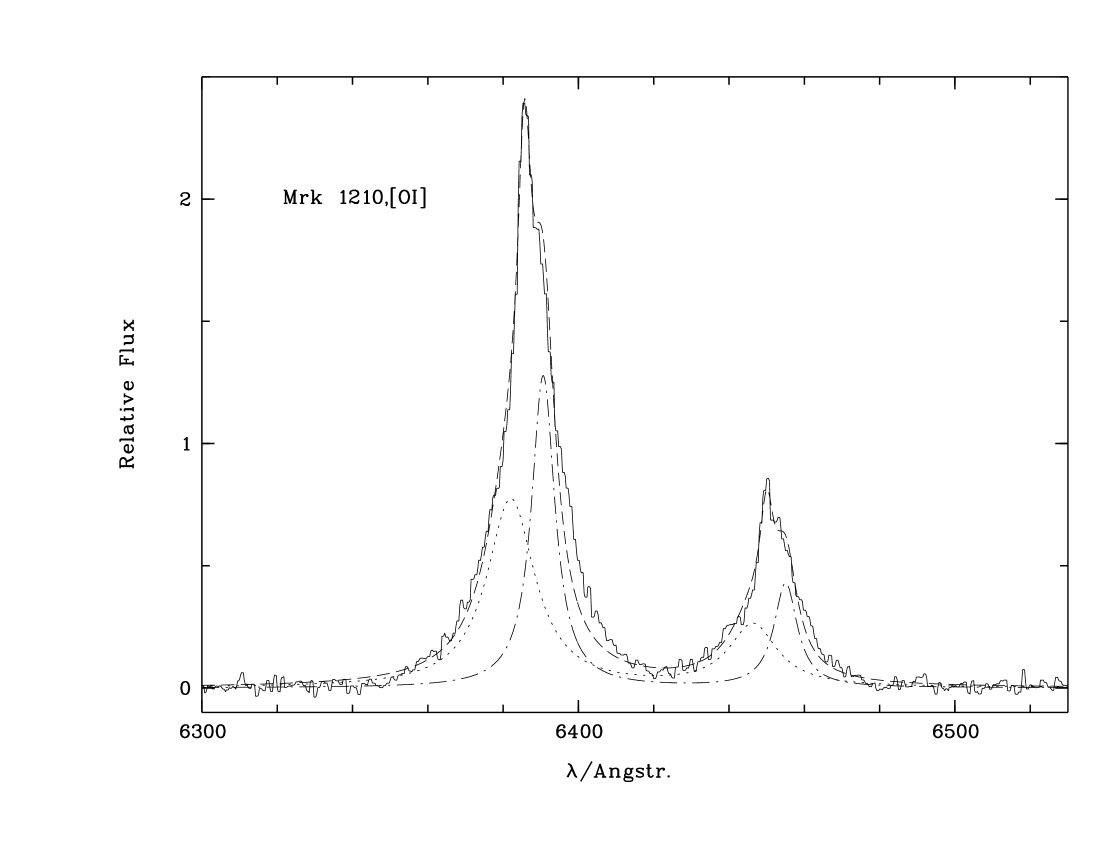
Figure 21: As in Fig. 20, but for [Oi]$\lambda\lambda 6300,6363$ from the maximal line-emitting 2″ of Mrk 1210.

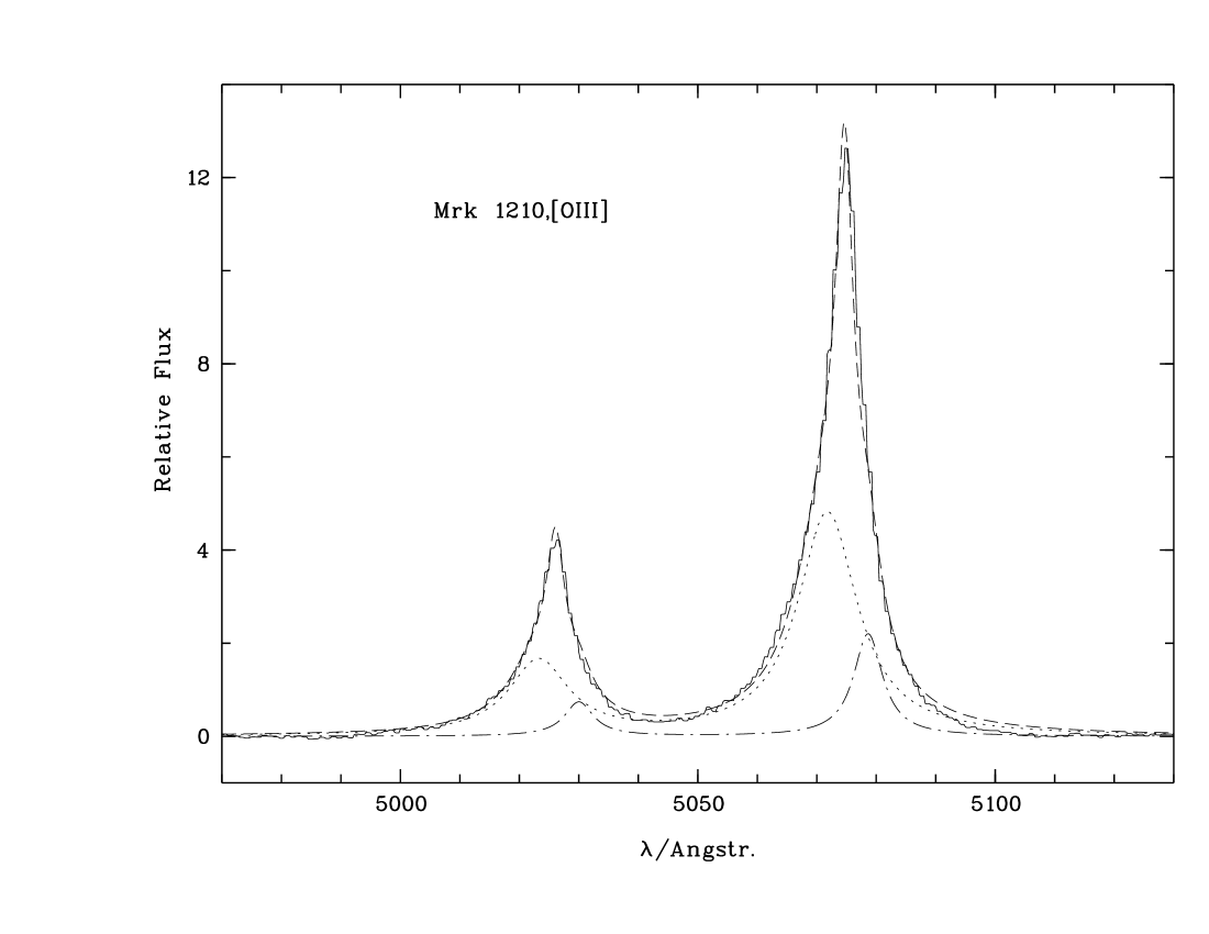
Figure 22: As in Fig. 20, but for [Oiii]$\lambda\lambda 4959,5007$ from the maximal line-emitting 2″ of Mrk 1210.

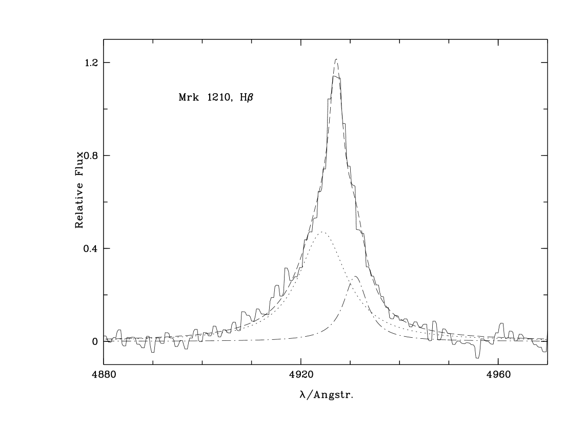
Figure 23: As in Fig. 20, but for H$\beta$ from the maximal line-emitting 2″ of Mrk 1210.

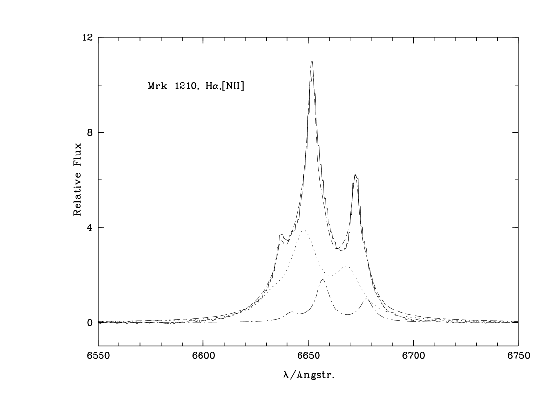
Figure 24: As in Fig. 20, but for H$\alpha$+[Nii] from the maximal line-emitting 2″ of Mrk 1210. In this special fit, the [Nii]/H$\alpha$ ratio is the same for systems $\cal{M}$, $\cal{B}$ and $\cal{R}$ (solution (1), see text for more details).

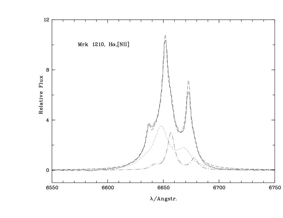
Figure 25: As in Fig. 24, but here the intensity ratios [Nii]/H$\alpha$ are allowed to differ among systems $\cal{M}$, $\cal{B}$ and $\cal{R}$ (solution (2), see text for more details).

5 Discussion

5.1 The narrow-line profiles of NGC 1052 and Mrk 1210

5.1.1 Kinematic bulk components

The slightly novel ansatz of the present work lies in the attempt to disentangle two to three emission-line systems from the observed line profiles. Ab initio such a task may be subject to pitfalls like non-uniqueness and particular care has to be devoted to the choice of a basic function that represents a single profile.

The above fitting experiments carried out with the spectra of NGC 1052 and Mrk 1210 showed that single-component fits as well as multi-component fits led to lower residuals and a lower number of fitting components when using Lorentzians as basic functions rather than the commonly employed Gaussians. The additional surprising effect of this choice was that we could essentially dispense with broad H$\alpha$ (and H$\beta$) components. There is no doubt that both galaxies display broad H$\alpha$ components in polarized flux but these are faint and are unlikely to be visible in spectra taken without a polarizing device.

If the Lorentzian decomposition is correct, the broad H$\alpha$ component extracted by Ho et al. (1997) in the total-flux spectrum of NGC 1052 has to be considered as spurious. Our alternative decomposition at least suggests to be cautious with claiming a broad H$\alpha$ component hidden in the H$\alpha$+[Nii] blend if it is only based on a mere decomposition in total flux. In this view it seems to be a coincidence that spectropolarimetry finally confirmed NGC 1052 as a LINER-1.

Before giving possible astrophysical settings for Lorentzian profiles, an empirical justification is in order. The significance of the decomposition into different Lorentzian components rests on the internal consistency achieved for all strong line profiles from H$\beta$ to [Sii]$\lambda 6731$. In particular, the same decomposition was employed for the collisionally excited transitions of [Oi], [Oiii], [Nii] and [Sii] as for the allowed recombination lines H$\alpha$ and H$\beta$. Because of electron densities believed to exceed $10^{9}$ cm^-3, a classical AGN BLR would only exhibit broad allowed lines (with line widths (FWHM) in the range $10^{3-4}$ km/s) so that we consider the components extracted here (with FWHM $\sim 10^{2-3}$ km/s) as belonging to parts of a NLR distinguished by different bulk motions.

Density tracers usually suggest densities in the range $10^{2-4}$  cm^-3 for the main components of NLRs. For NGC 1052 and Mrk 1210 blue components $\cal{B}$ with indications for rather high densities ($\sim 10^{6}$ cm^-3 or more) were isolated. In particular, $\cal{B}$ of Mrk 1210 hardly shows up in [Sii]$\lambda\lambda 6716,6731$, which suggests $n_{e}\gg 10^{3}$ cm^-3. However, since the critical densities of the well observed doublet [Nii]$\lambda\lambda 6548,6583$ are $\sim 10^{5}$ cm^-3, the latter value should not be exceeded by several orders of magnitude Furthermore, the trends shown in Komossa & Schulz (1997) indicate, that to boost [Nii]/H$\alpha$ relative to [Sii]/H$\alpha$ at high densities, a large ionizing input flux is necessary. $\cal{B}$ might therefore be an ‘ILR’ (intermediate-line region) with a density and a distance intermediate between the BLR and NLR. This designation is also supported by its large line width of 727 km/s, somewhat intermediate between a ‘typical’ NLR and a typical BLR.

In the early days of NLR analysis width-variations of narrow lines were frequently attributed to stratifications in velocity space observationally manifested via different critical densities or ionization potential (e.g. Pelat et al. 1981, Filippenko & Halpern 1984, Whittle 1985b, Schulz 1987). The decompositions proposed here explain different line widths by summing line components, each of constant width in velocity space, but different weighting for a component in each line. This assumption implies that each emission-line cloud emits all lines considered here, which will be the case when they are mainly ionization bounded.

While our data suggest that the $\cal{M}$ components arise in a rotating disk with ‘normal’ densities (their velocities fit the rotation curves), the $\cal{R}$ and $\cal{B}$ components appear to arise in bulk outflow systems.

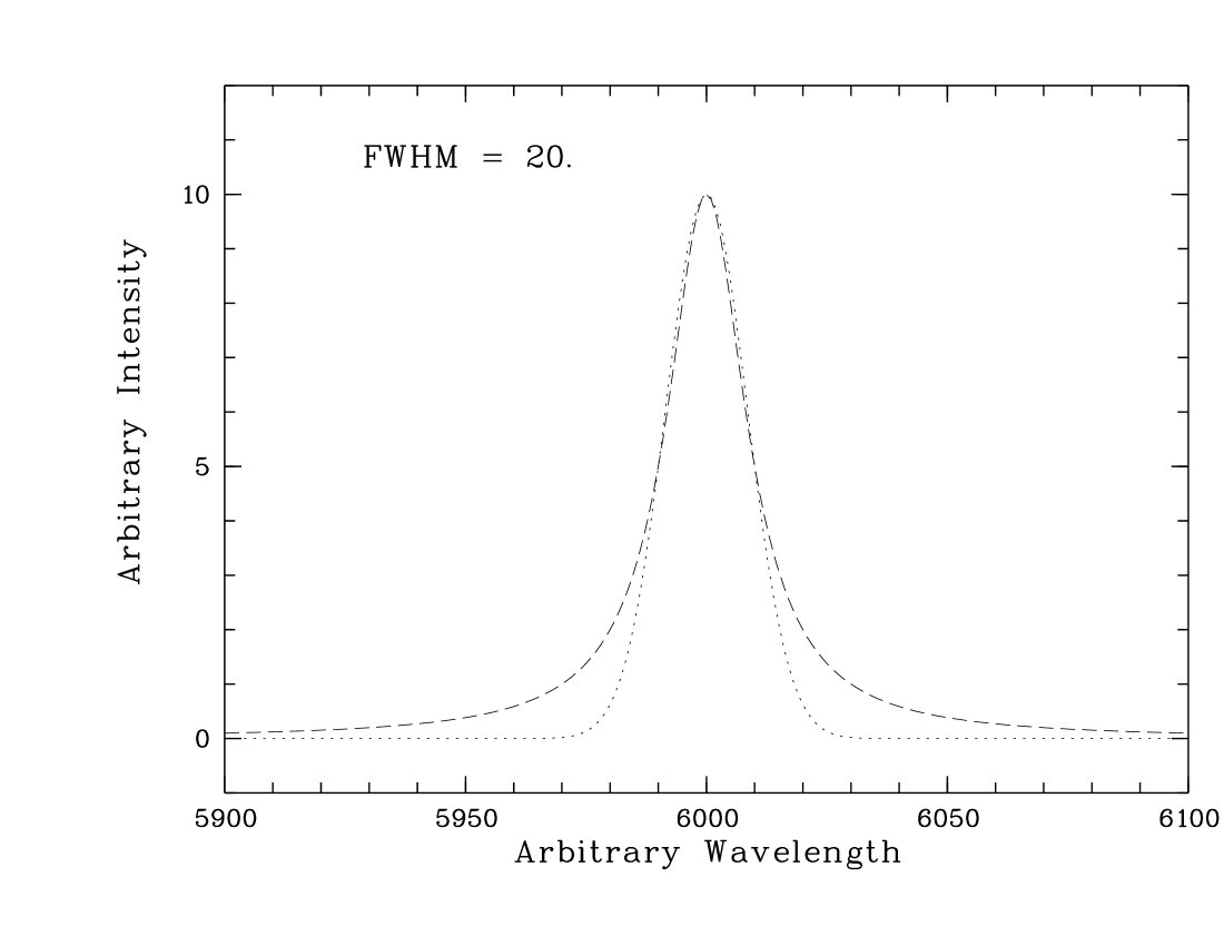
Figure 26: A Lorentzian (dashed) and a Gaussian (dotted) with same full width at half maximum.

5.1.2 Why Lorentzians?

Gaussians are relatively well suited to describe instrumental functions or thermal Doppler broadening or some kind of turbulence induced by random motions with Maxwellian-type velocity distributions. Lorentzians differ from Gaussians with same FWHM by a marginally narrower core and a slower fall-off to large velocities leading to more extended line wings (Fig. 26). The non-Gaussian nature of observed [Oiii] line profiles was early described by Whittle (1985a), who had noted that (i) “almost all the sample have [Oiii] profiles with a stronger base relative to the core than Gaussian” (his Sect. 5.3) and (ii) “the extreme wing widths (FWZI) usually lie in the range 1000–3000 km s^-1” (his Sect. 5.2).

For our line profiles, the observed line wings would have typically reached the noise levels at $\sim 6\%$ of the maximum. Eq. 1 implies that a Gaussian falls to 6.3% of the maximum at two HWHMs (half width at half maximum) from the center while a Lorentzian has decreased to 5.9% at four HWHMs. For components $\cal{M}$, $\cal{R}$ and $\cal{B}$ of Mrk 1210 described in Table 7 we get 4 HWHMs = $2\,w=416,700,1454$ km/s, respectively. How can such large velocities of $\sim 10^{2-3}$ km/s in the line wings be attained?

Turbulence of this order within the emission-line clouds would be strongly supersonic in gas with an observed temperature of $T\sim 10^{4}$ K, in which the characteristic thermal velocity and the velocity of sound are of the order of $\sim 10$ km/s. Hydrodynamic shocks would result in dissipation of the gained energy, most likely by radiation, perhaps contributing to, but not dominating the ionization equilibrium that is essentially governed by radiative input. To uphold the velocities, a strong steady mechanical energy input would be required.

Outflow velocities of the order of $10^{3}$ km/s have frequently been seen in AGN absorption lines. Elvis (2000) reviewed the observations and proposed an AGN-type-I unification scheme. Cloudlets comoving in a bipolar wind system might lead to such line wings whose width would strongly depend on the viewing angle of the system.

A less explored, albeit not far-fetched, mechanism to produce the line wings might be magneto-hydrodynamic waves that could mimick supersonic turbulence (Shu 1992).

A different type of alternative would be scattering of photons at fast particles. Dust particles are far too slow, but electrons in the cited photoionized clouds have velocities of $10^{3-4}$ km/s. Scattering of a line at these electrons could cause broad line wings via redistribution in frequency space. In the early times of AGN spectroscopy, this type of scattering was proposed to explain the widths of lines from the BLR (Weymann 1970; Mathis 1970). In a hotter intercloud medium with $T\sim 10^{6-8}$ K, which may confine the emission-line clouds by its thermal pressure, electrons can attain velocities of $10^{4-5}$ km/s. Shields & McKee (1981) suggested electron scattering in such a medium as an explanation for very broad H$\alpha$ wings observed in the quasar B 340. Their case could be transferred to the Lorentzian wings, if one sees only the ‘tip of the iceberg’ of hot-ISM scattering because otherwise the wings would have to be much wider.

The fraction of scattered flux is roughly given by the electron-scattering optical depth $\tau_{e}$ and the covering fraction of the scattering medium. Effective column-densities of fully ionized gas of $2\,10^{22}$ cm^-2 would be required to obtain electron-scattering optical depths on the percent level. Attributing such a column to a kpc-extended sphere of a hot intercloud medium would lead to a total bremsstrahlung luminosity (Eq. 5.15b in Rybicki & Lightman 1979) of $2.6\,10^{42}(n_{e}/10\,{\rm cm}^{-3})^{2}\sqrt{(T/10^{6}{\rm K})}(R/500{\rm pc})^{3}$ erg/s. This is a lower limit because the estimate neglects line emission. Thermal soft-X-ray emission is estimated to be $\sim 10^{40}$ erg/s for NGC 1052 (Weaver et al. 1999), and is measured to be $\sim 10^{41}$ erg/s in Mrk 1210 (Awaki et al. 2000). We conclude that we do not see a sufficient amount of hot coronal gas to produce the required wings. However, a viable alternative would be scattering at the cooler ($T\sim 10^{4}$ K) emission-line clouds with electron densities $\sim 10^{2-3}$. With a scale $R\approx 10^{2}$ pc and a geometrical scattering factor $f\approx 0.3$ one easily obtains a ratio of scattered luminosity to input luminosity $L_{\rm s}/L_{\rm in}=f\tau_{e}$ of a few percent, which suffices to explain th extended wings of the narrow lines.

5.1.3 Relationship to spectropolarimetry

Spectropolarimetry of NGC 1052 (Barth et al. 1999) and of Mrk 1210 (e.g. Tran 1995) provides direct evidence for scattering of the continuum and broad lines.

In Mrk 1210 the degree of polarization $P$ in the forbidden lines decreases significantly (to less than 1%; to $\sim 0$% in the cores of [Oiii]) compared to that of the continuum indicating that the main body of the narrow-line profiles is not scattered (this is the situation in many ‘hidden-Seyfert-1’ galaxies, which are thereby backing the unified model). In NGC 1052 there is hardly a decrease in the forbidden lines, suggesting that a major part of the forbidden-line profiles is scattered as well, rendering this object as an unusual ‘hidden-LINER-1’ object. How can these observations be reconciled with the line-profile decomposition proposed here? We discuss the galaxies in turn.

The average angle of polarization in Mrk 1210 is $\sim 30\degr$ (Tran 1995). This is 80° off from the kinematical major axis of the central kpc-disk (cf. Table 2), whose geometry is not favorable to give rise to polarized radiation because of its near-face-on view. A suggestive explanation is found by the observed shift of the line-continuum maximum by $\sim 1\arcsec$ to the west of the kinematical center (see Fig. 15, where the zero point of the abscissa is at the brightness maximum), which is consistent with a view that the true AGN is obscured and is situated at the kinematical center. Via some escape route AGN radiation reaches the brightness center, thereby giving rise to the polarized scattered broad-line wings and the polarized part of the continuum. In the AGN standard view, the high-excitation Seyfert-2 characteristics of the brightness center would be traced back to photoionizing AGN radiation reaching this region. Because the AGN continuum is only seen in scattered light and the stellar continua from the starburst plus the older stellar populations certainly dominate, it is not surprising that the precise amount of visible ‘featureless continuum’ is under debate (Schmitt et al. 1999).

In NGC 1052, Barth et al. (1999) found a polarimetric position angle of H$\alpha$ (+[Nii]) of 178°, which is neither aligned with – nor perpendicular to – the major axis of the gaseous disk (p.a. $\sim 45\degr$ following Davies & Illingworth (1986)). However, this apparently accreted narrow-line gas does not necessarily reflect the orientation of the ‘central machine’. If the kpc-radio structure detected by Wrobel (1984) can be identified with a jet perpendicular to the central accretion disk, the polarimetric p.a. would perfectly fit with the idea that the polarized component is scattered light originating in a nucleus obscured from direct view.

However, unlike in Mrk 1210 (Tran 1995; second panel in his Fig. 15), in NGC 1052 the degree of polarization $P$ (Barth et al. (1999); their Fig. 1, middle and lower panel, and Fig. 2, lower panel) only hardly decreases in the [Nii]+H$\alpha$ blend and shows upturns in [Oi] and [Sii]. Considerable noise and possible Galactic foreground polarization affecting the spectrum lets Barth et al. focus on [Oi]$\lambda 6300$, whose value of $P$ lies significantly above that of the continuum. In particular, they note that [Oi] is narrower in polarized light and that the [Oi]/[Sii] flux ratio is larger in Stokes flux than in total flux.

These latter findings resemble those we found for component $\cal{B}$ in NGC 1052 (cf. Table 5, last two rows). Relative to $\cal{A}$, in $\cal{B}$ usually [Oi] is stronger and [Sii] is weaker. The dense narrow-line gas of $\cal{B}$ could be (partially) hidden and its radiation be scattered like the broad polarized wings of H$\alpha$.

Alternatively, Barth et al. (1999) suggested transmission through a region of aligned dust grains as a possible mechanism for the [Oi] polarization. Indeed, Davies & Illingworth (1986) noted a dusty zone on the eastern side of the nucleus where component $\cal{B}$ is predominantly detected.

5.2 Relationship to H₂O megamaser activity

5.2.1 General aspects

The $\lambda$$\sim$1.3 cm transition of H₂O can be driven to mase by collisions, provided that the densities and temperatures are high enough ($\ga$10⁷ cm^-3 and $\ga$400 K; see Sect. 1). In galactic sources of water maser emission, namely in star forming regions, the necessary conditions can be produced by shock waves which provide not only proper physical conditions (e.g. Elitzur 1992, 1995) but also greatly enhanced H₂O abundances (e.g. Melnick et al. 2000). The unique association of H₂O megamasers with AGN and the fact that not all of the megamaser emission can arise from unsaturated amplification of an intense nuclear radio continuum (e.g. Greenhill et al. 1995a; AGN brightness temperatures can be much higher than $T_{\rm b}$$\la$10⁴ K, encountered in ultracompact galactic HII regions) indicates, however, significant differences between galactic maser and extragalactic megamaser sources. Possible scenarios that may produce suitable physical environments for luminous megamaser emission from the so-called ‘disk-masers’ (see Sect. 1) are (1) irradiation of dense warped disks by X-rays from the AGN (Neufeld et al. 1994), (2) shocks in spiral density waves of a self-gravitating disk (Maoz & McKee 1998) and (3) viscous dissipation within the accretion disk (Desch et al. 1998). For the so-called ‘jet-masers’, interaction of dense neutral gas with a radio jet is a viable scenario that may also yield temperatures of several 100 K and large H₂O abundances (Peck et al. 2001).

5.2.2 Outflow as H₂O maser trigger: winds of an AGN or a starburst?

In view of the overall angular scales, i.e. a few milliarcseconds for interferometric maps of 1.3 cm megamaser emission and a few arcseconds for our study, a connection between optical and radio data is difficult to establish. In elliptical galaxies the large scale dust lanes and nuclear jet orientation is correlated (e.g. Kotanyi & Ekers 1979; Möllenhoff et al. 1992). In Seyfert galaxies, however, large scale disks and nuclear disks tend to be inclined with respect to each other (e.g. Ulvestad & Wilson 1984). In some galaxies, the nuclear jet may be oriented not too far from the plane of the parent galaxy and may thus interact with molecular clouds, forming jet-masers off the very nuclear region (see e.g. Gallimore et al. 2001 for the case of NGC 1068). The near-to-face-on large scale view onto Mrk 1210 (Malkan et al. 1998) is thus not arguing against high shielding column densities along the line-of-sight toward the nucleus.

Radio jets may be a strong agent to drive maser action when hitting high-density clumps or entraining molecular gas (see Elitzur 1995 for physical processes involved). However, optically detectable ionized outflowing material, e.g. a magnetized wind from an accretion disk (cf. Krolik 1999) that would be less violent close to the equatorial plane than towards higher latitudes, may also be relevant. In systems with a nuclear thin disk and a thicker outer torus or in systems with misaligned angular momenta of nuclear and outer disk, a nuclear wind impinging on molecular clouds farther out appears to be an attractive alternative to the previously outlined jet-maser excitation scenario. As in the case of an interaction with a jet, shocks at speeds not destroying the dust grains and a warm (several 100 K) H₂O enriched postshock medium are expected. The spatial extent of the outflowing gas that may have a larger ‘cross section’ than the faster radio jet makes such an interaction particularly likely.

If one relies on outflow as one of the primary maser agents, it must be intriguing that H₂O megamasers have, until recently, only been detected in galaxies with AGN-typical features because large-scale winds and outflows are properties not only associated with AGN but also with starbursts. The key to this conundrum may be the fact that the sample of known H₂O megamaser sources is still rather small. Recently H₂O megamasers have been observed, for the first time, in starburst galaxies (Hagiwara et al. 2002; Peck et al. 2003) and for the ‘traditional’ absence of H₂O megamasers in type-1 AGN, proposed by Braatz et al. (1997), a first counterexample may have been found as well (see Nagar et al. 2002).

Below, some characteristic features of our four individual galaxies are briefly summarized.

5.2.3 Individual sources

In NGC 1052, a notable feature is the presence of a strong high-density outflow (Sect. 4.3.2). For this galaxy the (VLBA+VLA) observed maser sources are found to coincide with the innermost part of the southwestern radio jet rather than being related to the nearby putative nuclear disk (Claussen et al. 1998). The masers are redshifted by 80 to 200 km/s relative to $v_{\rm sys}$ as tabulated by de Vaucouleurs et al. (1991). The distance to the 43 GHz radio core, the supposed location of the central engine, is less than a milliarcsecond (0.07 pc).

Due to the spatial coincidence Claussen et al. (1998) suggested to relate the maser activity to the VLBI jet or to a fortuitously positioned foreground cloud that amplifies the radio continuum of the inner jet. The strong high-density outflow disentangled from the rotating disk (Sect.4̇.3.2) raises another alternative source to excite the maser activity. In this case the small solid angle of the inner jet, the presumably larger solid angle of the outflowing component and the location of the masers in front of the brightest parts of the jet suggest unsaturated H₂O emission amplifying the strong radio background.

Towards Mrk 1210, the brightness maximum BM of the emission-line region is rather compact (Falcke et al. 1998) and BM is slightly misplaced from the kinematical center. Strong radial flows in BM may be related to the flows that give rise to megamaser activity. No interferometric radio map of the H₂O emission has yet been published.

In IC 2560 and NGC 1386 we found little obvious evidence for outflow, presumably because of the near-edge-on view on these galaxies making a flow perpendicular to a disk hard to detect. The NGC 1386 line profiles show pronounced structure, and Rossa et al. (2000) isolated even more subtle substructures suggestive of non-circular motions like locally expanding gas systems. Such more localized flows could be related to megamaser activity as well. However, we caution that integrating over l.o.s., which intersect a dusty and patchy rotating disk, can well lead to bumpy line profiles. Interpreting such bumps by local Gaussians may be misleading. A meaningful discussion requires observations with significantly higher resolution and a detailed model of the dusty spiral disk. While the megamaser in IC 2560 may originate from a circumnuclear disk not related to outflowing gas (Ishihara et al. 2001), no high resolution H₂O map has yet been published from NGC 1386.

In passing, it should be noted that the mere presence of outflow in H₂O megamaser galaxies is not new. In much more detail outflow bulk systems were studied in the nearby galaxies M 51 (Cecil 1988) and NGC 4258 (Cecil et al. 2000), but a direct relationship to their megamaser activity (e.g. Herrnstein et al. 1999; Hagiwara et al. 2001) has so far been elusive. M 51 and NGC 4258 are likely not suitable candidates to prove such a relationship, but optical data with subarcsecond resolution are needed for a convincing demonstration in other sources.

6 Final conclusions

We have analyzed exploratory optical spectra of four H₂O megamaser galaxies in order to disentangle kinematically discernable bulk components of their emission-line regions. For each object we propose a model of the global kinematics. The gas dynamics in IC 2560 and NGC 1386 is mainly determined by gravitationally dominated motions in a disk. However, there is a bias due to the close-to-edge-on view onto their disks making minor-axis outflow hard to detect. For NGC 1052 and Mrk 1210 emission from gravity-dominated dynamics of orbiting clouds could be separated from that of systems being in outflow. Line-broadening within the individual bulk components appears to be characterized by scattering wings.

IC 2560 is a highly inclined Sb spiral with a nuclear high-ionization Seyfert-2 spectrum displaying relatively narrow (FWHM $\sim 200$ km/s on an arcsecond scale) emission lines from a central rotating disk. If its major-axis orientation and inclination agree with that of the outer galaxy, the core mass (radius 100 pc) will be $9\,10^{6}$ M_⊙, consistently larger than the $2.8\,10^{6}$ M_⊙, given by the orbital velocities of the maser sources presumably embedded in a compact disk of outer radius 0.26 pc as measured by Ishihara et al. (2001). A slight blueward asymmetry of the line profiles suggests the presence of outflow (Sect. 4.4.1, Fig. 3).

The nuclear mass of $\sim 10^{7}$ M_⊙ in IC 2560 appears to be rather small. It would be larger by a factor of 1.5 if a distance of 39 Mpc (see comment in Table 2) were adopted.

NGC 1386 is a highly inclined Sa spiral with a nuclear high-ionization Seyfert-2 spectrum displaying rather structured asymmetric emission-line profiles that we interpret as arising from various parts of a central edge-on orientated disk. We dismiss the term ‘radiation cone’ for this object because the elongated H$\alpha$ morphology may simply reflect the edge-on view on the matter-bounded disk. The morphology together with analogy reasoning suggests that the disk is a dusty gaseous mini-spiral, which appears to be warped. Its rotation curve inside a diameter of 1.6 kpc yields a dynamically acting mass of $\sim 5\,10^{9}$ M_⊙, while the visible line-emitting ionized gas has a mass of $\sim 10^{5-6}$ M_⊙, which is a very small fraction of the total mass of nuclear gas that is likely to be of the order of ten percent of the dynamical mass.

There is a lack of line emission from the kinematical center (the center of the disk), which is probably due to obscuration by an equatorial dust disk that is evidenced by a dust lane crossing the center. A slight east-west gradient in velocity arising in protrusions seen on an HST image (Ferruit et al. 2000) could be due to minor-axis outflow, i.e. a flow essentially perpendicular to the disk (Sect. 4.2.2).

AGN narrow-line emitting disks like in IC 2560 and NGC 1386 explain general findings that the widths of narrow-lines are broadly correlated with the nuclear stellar velocity dispersion (Nelson & Whittle 1996). Such NLRs are likely to be part of the nuclear gas-dust spirals commonly seen on HST images of AGN on a scale of $\sim 10^{3}$ pc (Malkan et al. 1998; Martini & Pogge 1999; Martini 2001). However, so far unobserved very narrow lines should be emitted from galaxies with central disks seen face-on, if NLRs were only dominated by disk dynamics. The other two (non-edge-on) galaxies provide examples for additional dynamical components.

NGC 1052 is an elliptical galaxy with a nuclear low-ionization emission line region (LINER). All major line profiles from the brightness center out to 2″ northeast can be decomposed into two components $\cal A$ and $\cal B$, each with the same width in velocity space for all lines at a given spatial position. $\cal A$ is attributed to a rotating disk, while $\cal B$ is blueshifted by $\sim 400$ km/s suggesting outflow of high-density gas relative to the disk. Line ratios of both $\cal A$ and $\cal B$ are LINER-like. We propose to relate $\cal B$ to the peculiar forbidden-line polarized component detected by Barth et al. (1999) (Sect. 5.1.3). A faint broad H$\alpha$ component, which is seen in polarized flux, is not required in total flux. The presence of strong high-density outflow suggests to explore the possibility whether such a flow could be an alternate trigger of the H₂O megamaser activity in NGC 1052.

Mrk 1210 is an amorphously looking Seyfert-2 galaxy that contains a nuclear kiloparsec-spiral seen face-on. A bright emission-line spot appears to be slightly shifted from the partially obscured kinematical center. In total (unpolarized) flux the emission from the bright spot can be decomposed into three narrow-line components $\cal M$ (the ‘normal’ main component), $\cal R$ (a redshifted component), and $\cal B$ (a blueshifted component) without any BLR component. $\cal M$ is tentatively attributed to the rotating spiral from which only a small velocity variation could be measured because of its near-face-on orientation. $\cal R$ and $\cal B$ are outflow components that may both be related to the cospatial starburst and to ionization by the active nucleus. The megamaser activity might be related to the outflow.

The line ratios from the bulk components of Mrk 1210 fall into the AGN regime of the VO diagrams. The shifts of component $\cal{R}$ (by 240 km/s to the red of $\cal{M}$) and of component $\cal{B}$ (by 169 km/s to the blue relative to $\cal{M}$) are moderate, but of significant influence because major portions of the emission-line region are involved. Regarding line widths and densities $\cal{B}$ shows characteristics of an intermediate-line-region between BLR and NLR (Sect. 5.1.1).

Finally, it should be noted that the successful line-profile decompositions rest on Lorentzians rather than Gaussians as basic functions. Hence, extended wings of intrinsic narrow-line profiles of the bulk components may not be uncommon. Crude estimates suggest that electron scattering at the ionized gas itself might lead to a viable explanation, but detailed modelling of such processes would be useful.

There exists a possible connection between optical and radio lines. It is suggested that nuclear outflows impinging onto dense molecular clouds may provide a suitable trigger for megamaser emission. If inner torus and outer disk are misaligned, such an interaction appears to be particularly likely. A convincing verification of such a scenario requires, however, optical spectroscopy with subarcsecond resolution.

Appendix A Extraction of emission lines

A line intensity is obtained by integrating over a line profile in a flux calibrated spectrum. Both this integration and any profile decomposition are usually carried out after having subtracted the template spectrum and, if this has not led to a ‘zero base line’, a normalizing continuum has been subtracted as well. The latter is defined by a spline fit through marks set with the mouse cursor. The subjectivity of this eye fit hardly affects our basic results which rely on strong lines. The second step is necessary in case of an inappropriate template and/or the presence of a nonstellar continuum.

For each object, we define the spatial ‘center’ of an emission line region by the intensity maximum of the emission lines. In all cases this center coincides with the maximum of the continuum between the lines within a small fraction of an arcsecond. This kind of center may not coincide with the kinematical center (usually the ’nucleus’ of a galaxy) derived from an assumed symmetry of the velocity curve.

In the main text, discussion of emission-line intensity ratios is largely confined to the diagnostic classifiers proposed by VO which do not require large and notoriously uncertain reddening corrections. Occasionally intensity ratios of the [Sii] pair $\lambda 6716$ and $\lambda 6731$ will be given, which may be converted into some kind of weighted mean of the electron densities in the emission-line gas via Fig. 5.3 in Osterbrock (1989).

Appendix B Common line-profile analysis procedures

In AGN even the ‘narrow’ lines show considerable profile structure if measured at sufficient resolution (Vrtilek & Carleton 1985; Whittle 1985a). When single-component Gaussian fits fail, commonly multi-component Gaussian fits are employed. However, our multi-component fitting experiments of the spectra from NGC 1052 and Mrk 1210 showed that in these cases Lorentzian functions $C(\Delta\lambda)$ (also called ‘Lorentzians’; $C$ stands for ‘Cauchy function’) appear to be better suited if one intends, applying Occam’s razor, to minimize the number of required components and parameters in a multi-function fit. This may not be generally true. An instructive case of an asymmetric line profile being Lorentzian on the blue side and Gaussian on the red side is given by IC 2560 (cf. Sect. 4.1).

In a crude picture, the basic kinematical configurations expected are rotating disks, cones of outflowing gas or expanding shells. As shown in Schulz et al. (1995), line-of-sight integrations through such configurations would neither yield Gaussians nor Lorentzians. However, Schulz et al. (1995) also showed that the spatial and spectral smearing by an instrumental function that is wide in comparison to kinematical gradients and the presence of strong random motions superposed on the systematic bulk motions will lead to profiles characterized by a more symmetric core-wing structure.

This case applies here because our spectral resolution of $\sim 100$ km/s and spatial resolution of $\sim(1-2)\arcsec$  leads to integration over relatively large cells of the phase space of a NLR. Hence, for finding bulk motion components experimental fits are carried out by making use of Gaussians and Lorentzians as basic functions.

Lorentzian and Gaussian functions are fixed in the MIDAS data reduction software by the three convenient parameters central line position $\lambda_{0}$ (so that $\Delta\lambda=\lambda-\lambda_{0}$), $w={\rm FWHM}$ = full width at half-maximum and $h$, the maximal value of the profile function:

$$C(\Delta\lambda) = \frac{h}{1+4\,\Delta\lambda^{2}/w^{2}}$$ (1)

$$G(\Delta\lambda) = h\exp\left(-\ln(2)\,(4\Delta\lambda^{2}/w^{2})\right)$$ (2)

The ratio of the intensities of lines arising from the same upper level is given by the ratio of the corresponding transition probabilities (taken from Tables 3.8 and 3.10 in Osterbrock (1989)). Therefore the fits of [Oiii]$\lambda\lambda 4959,5007$, [Oi]$\lambda\lambda 6363,6300$ and [Nii]$\lambda\lambda 6548,6583$ are constrained by fixing intensity ratios in the proportion 1:3 and by equalizing the FWHM $w$.

Aside from these constraints, the basic strategy of fitting the line profiles is to start with a minimal set of assumptions. At first it is attempted to fit each narrow line by a single Lorentzian function or a Gaussian. If this fails we look for features (shoulder, second peak, asymmetric wing) giving clues for the initial condition to start a fit with a second component. In case of success, this component (with same velocity width $w$, where ($w$ in km/s) = (c in km/s) $\times$ (FWHM in Å) / ($\lambda_{\rm line}$ in Å)) will be applied to the other strong lines. If the positions among different lines agree sufficiently well in velocity space, the fit is considered as a success. In case of Mrk 1210 a three-component fit turns out to be necessary for which the positions of the components are also fixed only leaving the component intensity as a free parameter in different lines.

In physical terms, a bulk-motion system would emit lines of approximately the same width if it is, e.g., composed of local emitters (with sharp lines compared to the spectral resolution), which are photoionized to such a depth that they emit all lines used in the analysis.

Component line widths (FWHM) will be given as measured, i.e. without correcting for our finite spectral resolution of 100 km/s. Applying the convolution theorem for two Gaussians, a measured FWHM of 200 km/s would be 14% too large, with a rapidly decreasing relative excess for larger FWHM (6% at 300 km/s; 2% at 500 km/s).

Appendix C The derivation of rotation curves

To fix notations and assumptions we briefly describe how rotational velocities are derived for inclined plane disks. The disk may recede with a heliocentric radial velocity $v_{\rm hel}^{\rm c}$. Firstly, coordinates $x$ and $y$ are defined in the sky plane, with their axes along the apparent major and minor axis, respectively. The corresponding coordinates in the galactic plane are $\xi=x$ and $\eta=y/\cos i$, where $i$ ist the galactic disk’s angle of inclination as measured from face-on. Galactocentric distances in the sky plane are $\rho=\sqrt{x^{2}+y^{2}}$ and correspond to galactocentric distances $R=\sqrt{\xi^{2}+\eta^{2}}=\sqrt{x^{2}+(y/\cos i)^{2}}$ in the plane of the galaxy. A polar angle $\Theta$ in the plane of the galaxy ($\cos\Theta=\xi/R$) corresponds to $\theta$ in the sky plane via $\cos\Theta=\cos i/\sqrt{(\cos i)^{2}+(\tan\theta)^{2}}$.

To obtain the observed line-of-sight velocity component $v^{\rm los}$ of a circular (rotational) velocity $v^{\rm rot}$ in the galactic plane, one first projects $v^{\rm rot}$ with $\Theta$ onto a direction parallel to the minor axis of the galaxy and then with $i$ onto the l.o.s. so that $v^{\rm los}=v^{\rm rot}\,\cos\Theta\,\sin i$ or, with the above relation between $\Theta$ and $\theta$ (and $v^{\rm los}=v_{\rm hel}^{\rm obs}-v_{\rm hel}^{\rm c})$ :

$$v^{\rm rot}=(v_{\rm hel}^{\rm obs}-v_{\rm hel}^{\rm c})\frac{\sqrt{(\cos i)^{2}+(\tan\theta)^{2}}}{\sin i\cos i}$$ (3)

- (1) Aaronson, M., Bothun, G.D., Cornell, M.E., et al. 1989, ApJ 338, 654
- (2) Antonucci, R. R, J. 1993, ARA&A 31, 473
- (3) Antonucci, R. R. J. & Miller, J. S. 1985, ApJ 297, 621
- (4) Awaki, H., Ueno, S., Taniguchi, Y. & Weaver, K. A. 2000, ApJ 542, 175
- (5) Barth, A. J., Filippenko, A. V. & Moran E.C. 1999, ApJL 515, L61
- (6) Bertola, F., Pizzella, A., Persic, M. & Salucci, P. 1993, ApJ 416, L45
- (7) Bowen, I. S. 1960, ApJ 132, 1
- (8) Braatz, J. A., Wilson, A. S. & Henkel, C. 1994, ApJ 437, L99
- (9) Braatz, J. A., Wilson, A. S. & Henkel, C. 1996, ApJS 106, 51
- (10) Braatz, J. A., Wilson, A. S. & Henkel, C. 1997, ApJS 110, 321
- (11) Cecil, G. 1988, ApJ 329, 38
- (12) Cecil, G., Greenhill L.J., DePree C.G., et al. 2000, ApJ 536, 675
- (13) Claussen, M. J. & Lo, K.-Y. 1986, ApJ 308, 592
- (14) Claussen, M. J., Heiligman, G. M. & Lo, K.-Y. 1984, Nat 310, 298
- (15) Claussen, M. J., Diamond, P. J., Braatz, J. A., Wilson, A. S., Henkel, C. 1998, ApJ 500, L129
- (16) Colbert, E. J. M., Baum, S. A., O’Dea, C. P. & Veilleux, S. 1997, ApJS 105, 75
- (17) Davies, R. L. & Illingworth, G. D. 1986, ApJ 302, 234
- (18) de Vaucouleurs, G., de Vaucouleurs, A., Corwin, H. G., et al. 1991, Third Reference Catalogue of Bright Galaxies (RC3) (New York: Springer-Verlag)
- (19) Desch, S. J., Wallin, B. K. & Watson, W.D. 1998, ApJ 496, 775
- (20) dos Santos, P. M. & Lépine, J. R. D. 1979, Nat 278, 34
- (21) Elitzur, M. 1992, ARA&A 30, 75
- (22) Elitzur, M. 1995, RevMexAA 1, 85
- (23) Elvis, M. 2000, ApJ 545, 63
- (24) Fairall, A. P. 1986, MNRAS 218, 453
- (25) Falcke, H., Wilson, A. S. & Simpson, S. 1998, ApJ 502, 199
- (26) Falcke, H., Henkel, C., Peck A. B., et al. 2000, A&A 358, L17
- (27) Ferruit, P., Wilson, A. S. & Mulchaey, J. 2000, ApJS 128, 139 (FWM2000)
- (28) Filippenko, A. V. & Halpern, J. P. 1984, ApJ 285, 458
- (29) Fosbury, R. A. E., Mebold, U., Goss, W. M. & Dopita M. D. 1978, MNRAS 183, 549
- (30) Gallimore, J. F., Henkel, C., Baum, S. A., et al. 2001, ApJ 556, 694
- (31) Gardner, F. F. & Whiteoak, J. B. 1982, MNRAS 201, 13p
- (32) Greenhill, L. J., Henkel, C., Becker, R., Wilson, T. L. & Wouterloot, J. G. A. 1995a, A&A 304, 21
- (33) Greenhill, L. J., Jiang, D. R., Moran, J. M., et al. 1995b, ApJ 440, 619
- (34) Greenhill, L. J., Gwinn, C. R., Antonucci, R. & Barvainis, R. 1996, ApJ 472, L21
- (35) Greenhill, L. J., Herrnstein, J. R., Moran J. M., Menten, K.M., Velusamy, T. 1997a, ApJ 486, L15
- (36) Greenhill, L. J., Moran, J. M. & Herrnstein J. R. 1997b, ApJ 481, L23
- (37) Greenhill, L. J., Ellingsen, S. P., Norris R. P., et al. 2002, ApJ 565, 836
- (38) Greenhill, L. J., Kondratko, P.T., Lovell, E.J., et al. 2003, ApJ, in press (astro-ph/0212038)
- (39) Hagiwara, Y., Kohno, K., Kawabe, R. & Nakai, N. 1997, PASJ 49, 171
- (40) Hagiwara, Y., Henkel, C., Menten, K. M. & Nakai, N. 2001, ApJ 560, L37
- (41) Hagiwara, Y., Diamond, P. J. & Miyoshi, M. 2002, A&A 383, 65
- (42) Haschick, A. D. & Baan W. A. 1985, Nat 314, 144
- (43) Heisler, C. A. & Vader J. P. 1994, AJ 107, 35
- (44) Henkel, C., Güsten, R., Downes, D., et al. 1984, A&A 141, L1
- (45) Henkel, C., Braatz, J. A., Greenhill, L. J. & Wilson, A. S., 2002, A&A 394, L23
- (46) Herrnstein, J. R., Moran, J. M., Greenhill, L. J., et al. 1999, Nat 400, 539
- (47) Ho, L. C., Filippenko, A. V., Sargent, W. L. W. & Peng, C. Y. 1997, ApJS 112, 391
- (48) Ishihara, Y., Nakai, N., Iyomoto, N., et al. 2001, PASJ 53, 215
- (49) Koekemoer, A. M., Henkel, C., Greenhill, L. J., et al. 1995, Nat 378, 697
- (50) Komossa, S. & Schulz, H. 1997, A&A 323, 31
- (51) Kotanyi, C. G. & Ekers, R. D. 1979, A&A 73, L1
- (52) Krolik, J. H. 1999, Active Galactic Nuclei: From the Central Black Hole to the Galactic Environment (Princeton, NJ: Princeton University Press)
- (53) Lequeux, J. 1983, A&A 125, 394
- (54) Malkan, M. A., Gorjian, V. & Tam R. 1998, ApJS 117, 25
- (55) Maoz, E. & McKee, C.F. 1998, ApJ 494, 218
- (56) Martini, P. 2001, ASP Conf. Proc. 249, The Central Kiloparsec of Starbursts and AGN: The La Palma Connection, eds. J.H. Knapen et al. (San Francisco), p98
- (57) Martini, P. & Pogge R.W. 1999, AJ 118, 2646
- (58) Mathewson, D. S., Ford, V. L. & Buchhorn, M. 1992, ApJS 81, 413
- (59) Mathis, J. S. 1970, ApJ 162, 761
- (60) Melnick, G. J., Ashby, M. L. N., Plume, R., et al. 2000, ApJ 539, L87
- (61) Miyoshi, M., Moran, J. M., Herrnstein, J. R., et al. 1995, Nat 373, 127
- (62) Möllenhoff, C., Hummel, E. & Bender, R. 1992, A&A 255, 35
- (63) Nagar, N. M., Oliva, E., Marconi, A., Maiolino, R. 2002, A&A 391, L21
- (64) Nelson, C. H. & Whittle, M. 1996, ApJ 465, 96
- (65) Neufeld, D. A., Maloney, P.R. & Conger, S. 1994, ApJ 436, L127
- (66) Oke, J. B. 1974, ApJS 27, 21
- (67) Osterbrock, D. E. 1989, Astrophysics of Gaseous Nebulae and Active Galactic Nuclei (Mill Valley, CA: University Science Books)
- (68) Peck, A. B., Falcke, H., Henkel, C. & Menten, K. M. 2001, ASP Conf. Proc. 249, The Central Kiloparsec of Starbursts and AGN, eds. J.H. Knapen et al. (San Francisco), p321
- (69) Peck, A. B., Tarchi, A., Henkel, C., et al. 2003, A&A, in preparation
- (70) Pelat, D., Alloin, D. & Fosbury, R. A. E. 1981, MNRAS 195, 787
- (71) Reunanen, J., Kotilainen, J. K. & Prieto, M. A. 2002, MNRAS 331, 154
- (72) Rossa, J., Dietrich, M. & Wagner, S. J. 2000, A&A 362, 501
- (73) Rybicki, G. B. & Lightman, A. P. 1979, Radiative Processes in Astrophysics (New York: John Wiley & Sons)
- (74) Schmitt, H. R., Storchi-Bergmann, T. & Fernandes, R. C. 1999, MNRAS 303, 173
- (75) Schulz, H. 1987, A&A 178, 7
- (76) Schulz, H. & Fritsch, Ch. 1994, A&A 291, 713
- (77) Schulz, H., Mücke, A., Boer, B., Dresen, M. & Schmidt-Kaler, Th. 1995, A&AS 109, 523 (SM95)
- (78) Schulz, H., Komossa, St., Schmitz, C. & Mücke, A. 1999, A&A 346, 764
- (79) Shields, G. A. & McKee, C. F. 1981, ApJ 246, L57
- (80) Shu, F. H. 1992, The Physics of Astrophysics II. Gas Dynamics (Mill Valley, CA: University Science Books)
- (81) Storchi-Bergmann, T., Fernandes, R. C. & Schmitt H.R. 1998, ApJ 501, 94
- (82) Tran, H. D. 1995, ApJ, 440, 578
- (83) Trotter, A. S., Greenhill, L. J., Moran J. M. et al. 1998, ApJ 495, 740
- (84) Tsvetanov, Z. I. & Petrosian, A. R. 1995, ApJS 101, 287
- (85) Tüg, H. 1977, ESO Messenger No. 11, p7
- (86) Tully, R. B. 1988, Nearby Galaxies Catalog (Cambridge: CUP)
- (87) Ulvestad, J. S. & Wilson, A. S. 1984, ApJ 285, 439
- (88) Veilleux, S. & Osterbrock, D. E. 1987, ApJS 63, 295 (VO)
- (89) Vrtilek, J. M. & Carleton, N. P. 1985, ApJ 294, 106
- (90) Weaver, K. A., Wilson, A. S. & Baldwin, J.A. 1991, ApJ 366, 50
- (91) Weaver, K. A., Wilson, A. S., Henkel, C. & Braatz, J. A. 1999, ApJ 520, 130
- (92) Weymann, R. J. 1970, ApJ 160, 31
- (93) Whittle, M. 1985a, MNRAS 213, 1
- (94) Whittle, M. 1985b, MNRAS 216, 817
- (95) Wrobel, J. M. 1984, ApJ 284, 531