The theoretical model of a magnetic white dwarf.

Abstract

In this paper a theoretical model of a magnetic white dwarf is studied. All numerical calculations are performed under the assumption of a spherically symmetric star. The obtained equation of state is stiffer for the increasing value of magnetic field \(B\). The numerical values of the maximum mass and radius are presented. Sensibility of the results to the choice of the magnetic field strength is evident. Finally the departure from the condition of isothermality of degenerated electron gas in gravitational field is discussed.

Department of Astrophysics and Cosmology, Institute of Physics, University of Silesia, Uniwersytecka 4, 40-007 Katowice, Poland.

1 Introduction

The possibility of the existence of white dwarfs with large magnetic fields was predicted by Blackett in 1947. Ever since Kemp et al. in their paper presented results of the first detection of magnetic white dwarfs, these kind of stars have been intensively studied (Kemp et al. 1970; Putney 1995; Reimers et al. 1996; Jordan 1992; Chanmugan 1992; Ostriker et al. 1968; Mathews et al. 2000). However, only a small minority (the exact percentage remains uncertain) of white dwarfs have detectable magnetic fields. The study of magnetic properties of white dwarfs are expected to provide information on the role played by magnetic fields in the stellar formation and the main sequence evolution. Magnetic fields in white dwarfs are interpreted as the relic of magnetic fields of their progenitors. Thus the evolution of the main sequence stars with fields of only a few Gauss leads to white dwarfs with weak magnetic fields which remain below the threshold detection. Magnetic Ap and Bp stars are considered themselves as progenitors of magnetic white dwarfs with the field strength $>100\,\,MG$.
The aim of this paper is to show how the assumption of finite temperature and nonzero magnetic field influences white dwarf parameters. In the presence of magnetic field the magnetic pressure which corresponds to the Lorence force has to be taken into account. However, its inclusion causes the deformation of a star from spherical configuration, (Konno et al. 1999). In this paper all calculations are performed with the assumption that the averaged value of the energy momentum tensor gives us the condition for small deformation of a star and allows to treat a star as a spherically symmetric one. This approximation is connected with the existence of the critical density $\rho_{\mathrm{crit}}$ below which a star became deformed. The gained results allow to construct the mass-radius relation for a white dwarf with the magnetic field and at finite temperature which has been chosen to be equal $10^{7}$ $K$. The description of the interior of a white dwarf has been made in terms of degenerate, uniform, isothermal, electron gas. Using the equation of state of classical gas the atmosphere model has been formulated. The atmosphere extent, luminosity, effective temperature and the value of the critical density $\rho_{\mathrm{crit}}$ as functions of the temperature, density and magnetic field strength have been examined. The determination of the critical point allows to neglect the deformation of the star and perform all calculations in the spherically symmetric approximation.
This paper is organized as follows.
Section 2 outlines the considered model and contains assumptions which are indispensable in determining the form of the energy momentum tensor and the value of the critical density $\rho_{\mathrm{crit}}$. In section 3 the numerical results and the discussion are presented.

2 The theoretical model of white dwarfs in the magnetic fields

This paper presents the theoretical model of a white dwarf in which the main contribution to the pressure which supports the star against collapse comes from ultra-relativistic electrons . The electrons are supposed to be degenerate with arbitrary degree of relativity $x=\frac{k_{\mathrm{F}}}{m_{\mathrm{e}}}$ (in this paper the units in which $c=\hbar=1$ were used ). The value of $x$ is a function of a density. Ions provide the mass of the star but their contribution to the pressure is negligible. The complete and more realistic description of a white dwarf requires taking into consideration not only the interior region of the star but also the atmosphere. The isothermal interior of a white dwarf is completely degenerated and covered by non-degenerate surface layer which is in radiative equilibrium. Thus the white dwarf matter consists of electrically neutral plasma which comprises positively charged ions and electrons.
The Lagrangian density function in this model can be represented as the sum

$${\mathcal{L}}={\mathcal{L}_{\mathrm{e}}}+{\mathcal{L}_{\mathrm{G}}}+{\mathcal{L}_{\mathrm{QED}}},$$ (1)

where ${\mathcal{L}_{\mathrm{e}}}$, ${\mathcal{L}_{\mathrm{G}}}$ describe the electron and gravitational terms, respectively. The ${\mathcal{L}_{\mathrm{QED}}}$ is the Lagrangian density function of the QED theory

$${\mathcal{L}_{\mathrm{QED}}}=-\frac{1}{4}F^{\mu\nu}F_{\mu\nu}.$$

The electron part of the Lagrangian is given by

$${\mathcal{L}_{\mathrm{e}}}=i\overline{\psi_{\mathrm{e}}}\gamma^{\mu}D_{\mu}\psi_{\mathrm{e}}-m_{\mathrm{e}}\overline{\psi_{\mathrm{e}}}\psi_{\mathrm{e}},$$

where $D_{\mu}$ is the covariant derivative defined as$\,\,D_{\mu}=\partial_{\mu}-ieA_{\mu}\,$ and $e$ is the electron charge. The Dirac equation for electrons obtained from the Lagrangian function ${\mathcal{L}}$ has the form

$$(i\gamma^{\mu}D_{\mu}-m_{\mathrm{e}})\psi_{e}=0.$$

The vector potential is defined as $A_{\mu}=\{A_{\mathrm{0}}=0,\,A_{\mathrm{i}}\}$ where

$$A_{\mathrm{i}}=-\frac{1}{2}\varepsilon_{\mathrm{ilm}}x^{\mathrm{l}}B_{\mathrm{0}}^{\mathrm{m}}.$$

The symmetry in which uniform magnetic field B lies along the z-axis has been chosen

$$B_{\mathrm{0}}^{\mathrm{m}}=(0,0,B_{\mathrm{z}}).$$

The energy momentum tensor is the sum of the perfect fluid part $T_{\mu\nu}^{\mathrm{matt}}$

$$T_{\mu\nu}^{\mathrm{matt}}=(\varepsilon+p)u_{\mu}u_{\nu}+g_{\mu\nu}p,$$

and the electromagnetic one $T_{\mu\nu}^{\mathrm{B}}$

$$T_{\mu\nu}^{\mathrm{B}}=F_{\mu}^{\lambda}F_{\nu\lambda}-\frac{1}{4}g_{\mu\nu}F_{\alpha\beta}F^{\alpha\beta}$$

and can be calculated taking the quantum statistical average

$$\bar{T}_{\mu\nu}=<T_{\mu\nu}>=T_{\mu\nu}^{B}+T_{\mu\nu}^{matt}.$$

In the cartesian coordinates the electromagnetic part of the energy momentum tensor in the flat space-time has the form

$$T_{\mu\nu}^{\mathrm{B}}=\left(\begin{array}[]{cccc}\frac{1}{2}B^{2}&0&0&0\\ 0&\frac{1}{2}B^{2}&0&0\\ 0&0&\frac{1}{2}B^{2}&0\\ 0&0&0&-\frac{1}{2}B^{2}\end{array}\right),$$ (2)

and presents the example of the anisotropic pressure. In general the pressure of the electron gas in the magnetic field can be written as the sum of two parts

$$P=P_{\mathrm{e}}+P_{\mathrm{QED}}$$

where $P_{\mathrm{e}}$ is the isotropic part of the pressure, $P_{\mathrm{QED}}$ can reach the value $\pm\frac{1}{2}B^{\mathrm{2}}$ and causes that the pressure became anisotropic. On the other hand $T_{{\mu}{\nu}}^{\mathrm{B}}$ for polar coordinates can be written as follows

$$\left(\begin{array}[]{cccc}\frac{1}{2}B^{2}&0&0&0\\ 0&-\frac{1}{2}B^{2}\cos 2\theta&\frac{1}{2}B^{2}r\sin 2\theta&0\\ 0&\frac{1}{2}B^{2}r\sin 2\theta&\frac{1}{2}B^{2}r^{2}\cos 2\theta&0\\ 0&0&0&\frac{1}{2}B^{2}r^{2}\sin^{2}\theta\end{array}\right).$$

Averaging over all directions allows to obtain the isotropic form of the energy momentum tensor relevant for the spherically symmetric configuration

$$\left(\begin{array}[]{cccc}\frac{1}{2}B^{2}&0&0&0\\ 0&\frac{1}{6}B^{2}&0&0\\ 0&0&\frac{1}{6}B^{2}&0\\ 0&0&0&\frac{1}{6}B^{2}\end{array}\right).$$

The assumption of the positivity of the total pressure $P$ has been made

$$P_{\mathrm{e}}-\frac{1}{2}B^{\mathrm{2}}\geq 0.$$

Any negative contribution to the pressure reduces it, gravity can not be compensated and this diminishes the radius of the star. The described above averaging approximates a star as a spherically symmetric object with the radius $R$ which is smaller than the equatorial radius of the anisotropic star. The case of an anisotropic star is calculated in details in the paper by Konno et al. (Konno et al. 1999). The condition of the positivity of the total pressure establishes a limiting value of the density noted $\rho_{\mathrm{crit}}$ or the critical point $x_{\mathrm{crit}}$ and puts limit on the spherically symmetric approximation (the deformation of the star is neglected). For densities smaller than the critical one the total pressure became negative and there is no gravity compensation in this direction.
The equations describing masses and radii of white dwarfs are determined by the proper form of the equation of state. The aim of this paper is to calculate the equation of state for the theoretical model of magnetic white dwarfs with the assumption of finite temperature.
Properties of an electron in the external magnetic field have been studied, for example by Landau and Lifshitz in 1938 (Landau et al. 1938). In this paper the effects of the magnetic field on an equation of state of a relativistic, degenerate electron gas is considered. The motion of free electrons in the homogeneous magnetic field of the strength $B$ in the direction perpendicular to the field is confined by the oscillatory force determined by the field $B$ and is quantized into Landau levels with the energy $nB$, $n=0,1,\ldots$. In the case of non-relativistic electrons their energy spectrum is given by the relation

$$E_{\mathrm{n,p}_{z}}=n\omega_{\mathrm{c}}+\frac{p_{\mathrm{z}}^{2}}{2m_{\mathrm{e}}}$$

where $n=j+\frac{1}{2}+s_{\mathrm{z}}$, the cyclotron energy $\omega_{c}=eB/m_{e}$, $p_{z}$ is the momentum along the magnetic field and can be treated as continuous. For extremely high magnetic field the cyclotron energy is comparable with the electron rest mass energy and this is the case when electrons became relativistic. Introducing the idea of the critical magnetic field strength $B_{\mathrm{c}}=m_{\mathrm{e}}^{2}/\mid e\mid$ which equals $4.414\times 10^{\mathrm{13}}$ $G$, it is easy to distinguish between non-relativistic and relativistic cases, for $B\geq B_{\mathrm{c}}$ the relativistic dispersion relation for the electron in the magnetic field is given by

$$E_{\mathrm{n,p}_{\mathrm{z}}}=\sqrt{p_{\mathrm{z}}^{\mathrm{2}}+m_{\mathrm{e}}^{\mathrm{2}}+2eB_{\mathrm{z}}n}$$ (5)

where $n$ is the Landau level, $p_{z}$ is the electron momentum along z-axis and $m_{e}$ is the rest mass of the electron. Along the field direction a particle motion is free and quasi-one-dimensional with the modified density of states given by a sum

$$2\int\frac{d^{\mathrm{3}}{p}}{(2\pi)^{\mathrm{3}}}\rightarrow 2\sum_{n=0}^{\infty}[2-\delta_{\mathrm{n0}}]\int\frac{eB_{\mathrm{z}}}{(2\pi)^{\mathrm{2}}}dp_{z},$$ (6)

$\delta_{\mathrm{n0}}$ denotes the Kronecker delta (Mathews et al. 2000). The spin degeneracy equals 1 for the ground ($n=0$) Landau level and 2 for $n\geq 1$. The redefined density of states makes the distinctive difference between the magnetic and non-magnetic cases. The equation (5) implies that for $n=0$, $E_{\mathrm{0}}=\sqrt{p_{\mathrm{z}}^{\mathrm{2}}+m_{\mathrm{e}}^{\mathrm{2}}}$ whereas for $n\geq 1$ $E_{n}=\sqrt{p_{\mathrm{z}}^{\mathrm{2}}+m_{\mathrm{e}}^{\star\mathrm{2}}}$. These relations indicate that the quantity $m_{e}^{\star}$ defined as $m_{\mathrm{e}}^{\star\mathrm{2}}=m_{\mathrm{e}}^{\mathrm{2}}+2eB_{\mathrm{z}}n$ can be interpreted as the effective electron mass which is different from the electron mass $m_{\mathrm{e}}$ for $n\geq 1$. The number density of electrons at zero temperature is given by the following relation

$$n_{\mathrm{e}}=\sum_{\mathrm{n=0}}^{n=n_{\mathrm{max}}}[2-\delta_{\mathrm{n0}}]2eB_{{z}}p_{\mathrm{e}}^{F}.$$

The maximum Landau level is estimated from the condition $(p_{\mathrm{e}}^{\mathrm{F}})^{\mathrm{2}}\geq 0$. One can define the critical magnetic density $\rho_{\mathrm{B}}$

$$\rho_{\mathrm{B}}=0.802\ Y_{\mathrm{e}}^{\mathrm{-1}}\gamma^{\mathrm{3/2}}g\,\,cm^{-3}$$ (7)

($\gamma=B_{{z}}/B_{{c}}$ means a dimensionless parameter which expresses the magnetic field strength through the value of the critical field $B_{{c}}$) for densities lower than $\rho_{\mathrm{B}}$ only the ground Landau level is present.
Assuming the finite temperature of the system which affects the electron motion in the external magnetic field the number density of electrons can be expressed now as

$$n_{\mathrm{e}}=\frac{2m_{\mathrm{e}}^{\mathrm{3}}\gamma}{4\pi^{\mathrm{2}}}\sum_{\mathrm{n=0}}^{\infty}[2-\delta_{\mathrm{n0}}]\times$$ (8)

$$(I_{\mathrm{0,0,+}}(z/t,1+2\gamma n)-I_{\mathrm{0,0,-}}(z/t,1+2\gamma n))$$

where the Fermi integral

$$I_{\lambda\mathrm{,}\eta\pm}(u,\alpha)=\int\frac{(\alpha+x^{2})^{\lambda\mathrm{/2}}x^{\eta}dx}{e^{\left(\sqrt{\alpha+x^{\mathrm{2}}}\mp u\right)}+1}$$ (9)

has been used. The $\mu_{\star}$ and $T_{\star}$ denote the chemical potential and temperature in the star interior and $z=\mu_{\star}/m_{\mathrm{e}}$, $t=k_{\mathrm{B}}T_{\star}/m_{\mathrm{e}}$, $u=z/t$ (Lai 2000; Bisnovatyi-Kagan 2000). Finite temperature together with decreasing value of the strength of the magnetic field tend to smear out Landau levels. The introduction of the concept of Fermi temperature

$$T_{\mathrm{F}}=E_{\mathrm{F}}/k_{\mathrm{B}}=(m_{\mathrm{e}}/k_{\mathrm{B}})\epsilon_{\mathrm{F}}\qquad(\mathrm{for}\rho<\rho_{\mathrm{B}}),$$ (10)

and the magnetic temperature

$$T_{\mathrm{B}}={\frac{\Delta E_{\mathrm{B}}}{k_{\mathrm{B}}}}$$ (11)

$$={\frac{m_{\mathrm{e}}}{k_{\mathrm{B}}}}\left(\sqrt{1+2n_{\mathrm{max}}\gamma+2\gamma}-\sqrt{1+2n_{\mathrm{max}}\gamma}\right)$$

where $\Delta E_{\mathrm{B}}$ is the energy difference between the $n_{\mathrm{L}}=n_{\mathrm{max}}$ level and the $n_{L}=n_{\mathrm{max}}+1$ level, is the convenient way for describing how the properties of free electron gas change at finite temperature and at the presence of the magnetic field. For $\rho=\rho_{\mathrm{B}}$ these temperatures equal $T_{\mathrm{F}}=T_{\mathrm{B}}$. The influence of the magnetic field is most significant for $\rho\leq\rho_{\mathrm{B}}$ and $T\leq T_{\mathrm{B}}$ when electrons occupy the ground Landau level. In this case one can deal with the strong quantizied gas and the magnetic field modifies all parameters of the electron gas. For example, for degenerate, non-relativistic electrons the pressure is proportional to $\rho^{\mathrm{3}}$ and this form of the equation of state which one can compare with that for the case B=0 for which $P\sim\rho^{\mathrm{5/3}}$. When $\rho>\rho_{\mathrm{B}}$ the Fermi temperature is still greater than the magnetic temperature $T_{\mathrm{B}}$. Electrons are degenerate and there are many Landau levels, now the level spacing exceeds $k_{\mathrm{B}}T$. The properties of the electron gas are only slightly affected by the magnetic field. With increasing temperature, there is the thermal broadening of Landau levels, when $T\geq T_{\mathrm{B}}$, the free field results are recovered. For $T\gg T_{\mathrm{B}}$ there are many Landau levels and the thermal widths of the Landau levels are higher than the level spacing. The magnetic field does not affects the thermodynamic properties of the gas (Lai 2000 ).
The total pressure of the system can be described as the sum of the pressure coming from electrons and ions plus small corrections coming from the magnetic field

$$P=P_{\mathrm{e}}+P_{\mathrm{QED}}.$$

The contributions from the same constituents form the energy density

$$\varepsilon=\varepsilon_{\mathrm{ion}}+\varepsilon_{\mathrm{QED}},$$

where $P_{\mathrm{QED}}=\frac{1}{6}B^{\mathrm{2}}$, $\varepsilon_{\mathrm{QED}}=\frac{1}{2}B^{\mathrm{2}}$. The electron pressure is defined with the use of the Fermi integral

$$P_{\mathrm{e}}=\frac{2\gamma m_{\mathrm{e}}^{\mathrm{4}}}{4\pi^{\mathrm{2}}}\sum_{n=0}^{\infty}[2-\delta_{\mathrm{n0}}]\times$$ (12)

$$I_{\mathrm{-1,2,+}}(z/t,1+2\gamma n)+I_{\mathrm{-1,2,-}}(z/t,1+2\gamma n)).$$

The ion energy density has the simple form

$$\varepsilon_{\mathrm{ion}}=\left(\frac{A}{Z}\right)n_{\mathrm{e}}m_{\mathrm{B}},$$ (13)

where $m_{\mathrm{B}}$ is the baryon mass. The ions are very heavy and are treated as classical gas. The influence of the magnetic field for ions is very small and this correction to the equation of state has been neglected.
The pressure and energy density dependence on the chemical potential $\mu_{\star}\,\,$ determines the form of the equation of state, which is calculated in the flat Minkowski space time. The obtained form of the equation of state is the fundamental input in determining macroscopic properties of a star. Outside the static spherically symmetric body the metric has the form

$$ds^{\mathrm{2}}=e^{\nu\mathrm{(r)}}dt^{\mathrm{2}}-e^{\lambda\mathrm{(r)}}dr^{\mathrm{2}}-r^{\mathrm{2}}d\theta^{\mathrm{2}}-r^{\mathrm{2}}\sin^{\mathrm{2}}\theta d\varphi^{\mathrm{2}},$$

where $\nu(r)$ and $\lambda(r)$ are metric functions. The covariant components of the metric tensor

$$g_{\mu\nu}=\left(\begin{array}[]{cccc}e^{\nu}&0&0&0\\ 0&-e^{\lambda}&0&0\\ 0&0&-r^{\mathrm{2}}&0\\ 0&0&0&-r^{\mathrm{2}}sin^{\mathrm{2}}\theta\end{array}\right).$$ (14)

together with the specified form of the energy momentum tensor $T_{\mu\nu}$ allows to derive the structure equations of a spherically symmetric star (Tolman Oppenheimer Volkoff equations)

$$\frac{dP(r)}{dr}=$$ (15)

$$= -\frac{G}{r^{\mathrm{2}}}(\rho(r)+P(r))\frac{(m(r)+4\pi P(r)r^{\mathrm{3}})}{(1-\frac{2Gm(r)}{r})}$$

$$\frac{dm(r)}{dr}=4\pi r^{\mathrm{2}}\rho(r).$$ (16)

As the solution the mass-radius relation for white dwarfs is obtained.
The analyzed model of the white dwarf has to include both the core of degenerate isothermal electrons and the atmosphere where the temperature changes with the radius. In this case the equation of hydrostatic equilibrium has to be supplemented by the transport equation

$$\frac{d(e^{\nu\mathrm{(r)}}T)}{dr}=-\frac{3}{16\sigma}\frac{\kappa\rho}{T_{\star}^{\mathrm{3}}}\frac{L}{4\pi r^{\mathrm{2}}}\frac{e^{\nu\mathrm{(r)}}}{\sqrt{1-\frac{2Gm}{r}}},$$ (17)

where $e^{\nu\mathrm{(r)}}$ is the redshift, $L$ is the luminosity, $\kappa$ is the opacity of the stellar material and $\sigma$ is the Boltzmann constant. After neglecting small corrections coming from the general relativistic form of the equation (17) and using the condition of isothermality $T_{\star}=const$ it is possible to determine the luminosity of a white dwarf. In the result the total radius of a white dwarf can be obtained from the relation

$$R=\left(\frac{1}{R_{\star}}-\frac{T_{\star}}{GM}\frac{k_{\mathrm{B}}}{\widetilde{\mu}}4.25\right)^{\mathrm{-1}},$$ (18)

( Shapiro et al. 1983 ). In this relation $R_{\star}$ is the core radius and $\widetilde{\mu}$ is the molecular weight of the gas particles. The boundary conditions for the equation (15) are giving in the following form: $P(r=0)=P_{\mathrm{c}}=P(\rho_{\mathrm{c}})$ where $\rho_{\mathrm{c}}$ denotes the density at the center of the star which in this paper ranges from $10^{\mathrm{5}}$ $g$ $cm^{\mathrm{-3}}$ to $10^{\mathrm{11}}$ $g$ $cm^{\mathrm{-3}}$. The condition $P(r=R)=0$ determines the star radius $R$. For such boundary conditions the value of the magnetic field and temperature are limited to the following values $T=0-10^{\mathrm{7}}$ $K$, $\gamma=0-0.1$, respectively. The results are presented in figures 1-3.
Studying the properties of a star in the framework of the general-relativistic Thomas-Fermi model one can made the assumption that the temperature and chemical potential are metric dependent local quantities and the gravitational potential instead of Poisson’s equation satisfies Einstain’s field equations. The energy momentum conservation $T_{;\nu}^{\mu\nu}=0$ which for spherically symmetric metric (LABEL:tensor_metryczny2) can be written as

$$\frac{d\nu}{dr}=-\frac{2}{P+\rho}\frac{dP}{dr}$$ (19)

together with the Gibbs-Duhem relation and with the assumption that the heat flow and diffusion vanishes, (Israel 1976) give the condition

$$\frac{\mu_{\star}}{T_{\star}}=const.$$ (20)

This implies that the temperature and chemical potential become local metric functions

$$T(r) = e^{\mathrm{-}\nu\mathrm{(r)/2}}T_{\star}$$ (21)

$$\mu(r) = e^{\mathrm{-}\nu\mathrm{(r)/2}}\mu_{\star}$$ (22)

where $T_{\star}$ and $\mu_{\star}$ are constant. The first equation in (21) is the well known Tolman condition for thermal equilibrium in a gravitational field, (Tolman 1934). Now, the Fermi-Dirac distribution function has to be redefined and is given in the following form

$$\frac{1}{e^{\left(\sqrt{1+x^{\mathrm{2}}+2\gamma n}-z_{\mathrm{0}}\right)/\mathrm{t}_{\star}}+1}\rightarrow\frac{1}{e^{\left(e^{\nu\mathrm{(r)/2}}\sqrt{1+x^{\mathrm{2}}+2\gamma n}-z_{\mathrm{0}}\right)/\mathrm{t}_{\star}}+1}$$

$$=\frac{1}{e^{\left(\sqrt{1+x^{\mathrm{2}}+2\gamma n}-z(r)\right)/\mathrm{t(r)}}+1},$$

( Bilić et al. 1999). In the result instead of the OTV equilibrium equations together with the equation of state which has been calculated in the flat space-time one can derived three self-consistent equations (15,16,19). These equations together with the local form of the equation of state are now functions of $r$. This is of particular importance in the case of strong gravitational fields.

3 Discussion

In order to construct the mass-radius relation for white dwarfs the proper form of the equation of state have to be enumerated. For our needs we have chosen the plasma as the main constituent of the theoretical model of the white dwarf interior. All calculations have been performed at finite temperature and different from zero magnetic field and compared with those of zero temperature and without magnetic field.
In Fig. 1 the applied forms of the equations of state for magnetic and non-magnetic white dwarfs have been presented. Dots indicate the location of critical points. The approximation of spherical symmetry can be used for densities grater than the critical one $\rho_{crit}$. The inclusion of the magnetic field makes the equation of state stiffer. In the case of zero temperature model there are clearly visible Landau levels which became smear out when the finite temperature is included. The figure in the subpanel shows the equation of state obtained for the low density range for the zero temperature case, Landau levels are visible. In Fig. 2 the mass-radius relations for magnetic white dwarfs are presented. For each value of $\gamma$ the maximum mass has nearly the same value however the approximation of spherical symmetry which is connected with the existence of critical point determines the configuration with maximum radius. For the sake of completeness this figure includes also the mass-radius relation obtained for the equation of state of Hamada and Salpeter (Hamada et al. 1961). The solid line represents the nonmagnetic case which has been get with the use of the Hamada Salpeter equation of state. Dashed and dotted curves have been constructed for different values of the magnetic field strength. The differences between these curves are very small. The most important effect concerns the position of the critical points connected with the applied approximation of the spherical symmetry. In this approximation stable white dwarf configurations exist only for densities higher then $\rho_{crit}$. Thus the critical points on the curves determine configurations with maximal radius $R$. The stronger the magnetic field the smaller the white dwarf radius is. The most extended objects are obtained for the weakest magnetic fields. Using the Thomas-Fermi approximation one can obtain the result in which the star interior is no longer isothermal. The temperature profiles are presented in Fig. 3 for the fixed values of the central density $\rho_{\mathrm{c}}$. The temperature has been changed but not in a significant way. This is in agreement with the value of the gravitational potential which in the case of white dwarfs is much smaller than that obtained for neutron stars. The higher the central density the more visible are changes in temperature inside the star. For the central density $\rho_{\mathrm{c}}=10^{\mathrm{10}}gcm^{\mathrm{-3}}$ the temperature difference in the center of the star equals $6\,10^{\mathrm{4}}$ $K$. The magnetic temperatures $T_{\mathrm{B}}$ for different values of the central density $\rho_{\mathrm{c}}$ and different magnetic field strengths are presented in Tables 1, 2, 3. It has been found that $T_{\mathrm{B}}$ increases with the increasing value of the magnetic field and decreasing for increasing value of the central density. In Tables 4, 5, 6 the basic parameters of magnetic and non-magnetic white dwarfs are collected. For the maximum mass configurations the atmosphere extent drop with the increasing strength of the magnetic field. The effective temperature rises with the increasing magnetic field whereas the luminosity is altered insignificantly. All changes of white dwarf parameters are evident in the area of moderate densities. In this paper a magnetization ${\mathcal{M}}$ in the medium is not included. The inclusion of magnetization changes the perpendicular to the magnetic field component of a pressure and alters the value of the star radius. In the paper by Felipe it is stated that for positive magnetization the transversal pressure exerted by the charged particles in the magnetic field is smaller than the longitudinal one by the amount $B{\mathcal{M}_{\mathrm{e}}}$ (Felipe et al. 2002). Thus for $n=0$ (the ground Landau level) $P_{\perp}=0$. The vanishing of the pressure means that the instability which leads to the gravitational collapse appear. However, considering the case of finite temperature it is necessary to take into account a fact that the temperature smearing out Landau levels causes the appearance of the residual pressure which supports the star against gravitational collapse. The instability criterion given by the condition

$$n_{\mathrm{max}}\simeq 2\,10^{\mathrm{-21}}\frac{n_{\mathrm{e}}^{\mathrm{2}}}{B_{\mathrm{z}}^{\mathrm{3}}}$$

sets in for densities equal $5.7\times 10^{\mathrm{3}}$ $g\,\,cm^{\mathrm{-3}}$ for $\gamma=0.01$, $5\times 10^{\mathrm{4}}$ $g\,\,cm^{\mathrm{-3}}$ for $\gamma=0.05$ and $1.5\times 10^{\mathrm{5}}$ for $\gamma=0.1$. This instability leads to a cigar like object whereas in the case considered in this paper gives in the limiting case a toroidal star.

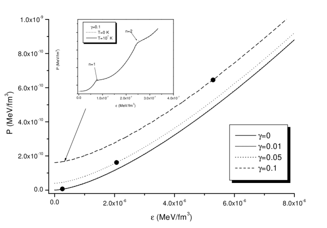
Figure 1: The equation of state for different cases of temperature and magnetic field strength. Dots represent the position of critical points. The figure in the subpanel depicts the form of the equation of state constructed for the low density range with clearly visible Landau levels.

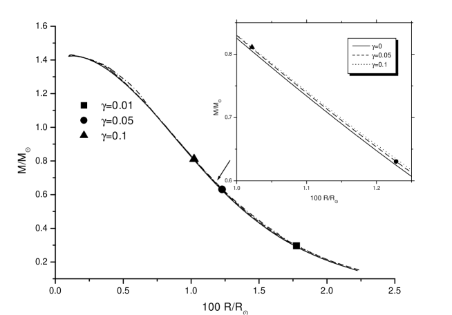
Figure 2: The mass-radius relations for magnetic white dwarfs obtained for different values of the magnetic field strength. The marked points represent the limiting values of radii for stable spherically symmetric configurations. The figure in the subpanel shows the mass-radius relations obtained for the radius range $1-1.25\,R_{\odot}/100$. For comparison the nonmagnetic case is constructed for the Hamada-Salpeter equation of state (Hamada et al. 1961).

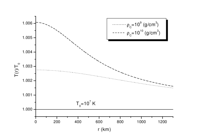
Figure 3: The temperature profile for different central densities.

$\rho_{\mathrm{c}}\,[g\,\,cm^{\mathrm{-3}}]$	$T_{\mathrm{B}}\,[K]$
$7\,10^{\mathrm{6}}$	$3.2398\,10^{\mathrm{7}}$
$3\,10^{\mathrm{7}}$	$2.2115\,10^{\mathrm{7}}$
$3.5\,10^{\mathrm{10}}$	$2.2631\,10^{\mathrm{6}}$

Table 1: The magnetic temperature $T_{\mathrm{B}}$ for the white dwarf with $\gamma=0.01$ and temperature $T=0$.

$\rho_{\mathrm{c}}\,[g\,\,cm^{\mathrm{-3}}]$	$T_{\mathrm{B}}\,[K]$
$7\,10^{\mathrm{6}}$	$1.6199\,10^{\mathrm{8}}$
$3\,10^{\mathrm{7}}$	$1.1088\,10^{\mathrm{8}}$
$3.5\,10^{\mathrm{10}}$	$1.1315\,10^{\mathrm{7}}$

Table 2: The magnetic temperature $T_{\mathrm{B}}$ for the white dwarf with $\gamma=0.05$ and temperature $T=0$.

$\rho_{\mathrm{c}}\,[g\,\,cm^{\mathrm{-3}}]$	$T_{\mathrm{B}}\,[K]$
$7\,10^{\mathrm{6}}$	$3.2647\,10^{\mathrm{8}}$
$3\,10^{\mathrm{7}}$	$2.2255\,10^{\mathrm{8}}$
$3.5\,10^{\mathrm{10}}$	$2.2632\,10^{\mathrm{7}}$

Table 3: The magnetic temperature $T_{\mathrm{B}}$ for the white dwarf with $\gamma=0.1$ and temperature $T=0$.

$1$	$2$	$3$	$4$	$5$	$6$
$1.083$	$1.099$	$0.0158$	$13679$	$-$	$0$
$1.089$	$1.105$	$0.0159$	$15822$	$4.6\,10^{\mathrm{5}}$	$0.01$
$1.087$	$1.103$	$0.0154$	$15896$	$3.6\,10^{\mathrm{6}}$	$0.05$
$-$	$-$	$-$	$-$	$-$	$0.1$

Table 4: The parameters of the magnetic and non-magnetic white dwarf with the mass $0.74$ $M_{\odot}$, central density $\rho_{\mathrm{c}}=7\,10^{\mathrm{6}}g\,\,cm^{\mathrm{-3}}$ and luminosity $L=0.0012$ $L_{\odot}$.

$1$	$2$	$3$	$4$	$5$	$6$
$0.807$	$0.815$	$0.00870$	$24633$	$-$	$0$
$0.810$	$0.818$	$0.00877$	$30799$	$4.6\,10^{\mathrm{5}}$	$0.01$
$0.809$	$0.818$	$0.00875$	$30864$	$3.6\,10^{\mathrm{6}}$	$0.05$
$0.807$	$0.816$	$0.00872$	$30991$	$9.4\,10^{\mathrm{6}}$	$0.1$

Table 5: The parameters of the magnetic and non-magnetic white dwarf with the mass $1$ $M_{\odot}$, central density $\rho_{\mathrm{c}}=3\,10^{\mathrm{7}}g\,\,cm^{\mathrm{-3}}$ and luminosity $L=0.0016$ $L_{\odot}$.

$1$	$2$	$3$	$4$	$5$	$6$
$0.130$	$0.130$	$0.00022$	$940946$	$-$	$0$
$0.117$	$0.117$	$0.00018$	$1.60\,10^{\mathrm{6}}$	$4.6\,10^{\mathrm{5}}$	$0.01$
$0.117$	$0.117$	$0.00018$	$1.61\,10^{\mathrm{6}}$	$3.6\,10^{\mathrm{6}}$	$0.05$
$0.111$	$0.111$	$0.00016$	$1.78\,10^{\mathrm{6}}$	$9.4\,10^{\mathrm{6}}$	$0.1$

Table 6: The parameters of the magnetic and non-magnetic white dwarf with the mass $1.42$ $M_{\odot}$, central density $\rho_{\mathrm{c}}=3.5\,10^{\mathrm{10}}g\,\,cm^{\mathrm{-3}}$ and luminosity $L=0.0023$ $L_{\odot}$.

The numbers from 1 to 6 denote:
1-the core radius of the white dwarf $100R_{\star}/R_{\odot}$
2-the total radius of the white dwarf $100R/R_{\odot}$
3-the extent of the atmosphere $100\Delta R/R_{\odot}$
4-the effective temperature $T_{\mathrm{eff}}$ $[K]$,
5-the critical density $\rho_{\mathrm{crit}}$ $[g\,\,cm^{\mathrm{-3}}]$,
6-the strength of magnetic field $\gamma$

References

- [1] Bilić, N., Viollier, R. D.: 1999, Gen.Rel.Grav. 31 1105-1113
- [2] Bisnovatyi-Kagan, G. S.: 2000
- [3] Chanmugan, G.: 1992, ARA& A 30 143
- [4] Felipe, R. G., Cuesta, H. J., Martinez, A. P., Rojas, H. P., Preprint astro-ph/0207150, Quantum instability of magnetized stellar objects
- [5] Hamada, T., Salpeter, E. E.: 1961 Astrophys. J. 134 683
- [6] Israel, W.:1976, Ann. Phys. 100 310
- [7] Jordan, S.: 1992, A & A 265 570
- [8] Kemp, J. C., Swedlund, J. B., Landstreet, J. D., Angel, J. R. P.: 1970, ApJ L77 161
- [9] Konno, K., Obata, T., Kojima, Y.: 1999, A & A 352 211-216
- [10] Lai, D.:2001, Rev. Mod. Phys. 73 629-661
- [11] Landau, L. D., Lifshitz, E. M.: 1938
- [12] Ostriker, J. P., Hartwick, F. D. A.: 1968, ApJ 153 797
- [13] Putney, A.: 1995, ApJ L67 451
- [14] Reimers, D., Jordan, S., Koester, D., Bade, N., Köhler, Th., Wisotzki, L.: 1996, A & A 311 572
- [15] Shapiro, S. L., Teukolsky, S. A., 1983 Black hols, white dwarfs and neutron stars New Yor
- [16] Suh, In-Seang, Mathews, G. J.: 2000, ApJ 530 949
- [17] Tolman, R. C.: 1934