Features of Muon Arrival Time Distributions of High Energy EAS at Large Distances From the Shower Axis

Abstract

In view of the current efforts to extend the KASCADE experiment (KASCADE-Grande) for observations of Extensive Air Showers (EAS) of primary energies up to 1$\cdot 10^{18}$ eV, the features of muon arrival time distributions and their correlations with other observable EAS quantities have been scrutinised on basis of high-energy EAS, simulated with the Monte Carlo code CORSIKA and using in general the QGSJET model as generator. Methodically various correlations of adequately defined arrival time parameters with other EAS parameters have been investigated by invoking non-parametric methods for the analysis of multivariate distributions, studying the classification and misclassification probabilities of various observable sets. It turns out that adding the arrival time information and the multiplicity of muons spanning the observed time distributions has distinct effects improving the mass discrimination. A further outcome of the studies is the feature that for the considered ranges of primary energies and of distances from the shower axis the discrimination power of global arrival time distributions referring to the arrival time of the shower core is only marginally enhanced as compared to local distributions referring to the arrival of the locally first muon.

1 Introduction

Since the first experimental studies in 1953 by Bassi, Clark and Rossi [1] and Jelley and Whitehouse [2] arrival time distributions of the charge particle components of Extensive Air Showers (EAS) have been often theoretically and experimentally investigated under various aspects [3, 4, 5, 6, 7, 8, 9]. Systematic studies are performed particularly at large EAS detector installations: in Haverah Park [10, 11, 12, 13, 14, 15, 16], at the Potchefstroom University [17], in Akeno and on Mt. Chacaltaya [18, 19, 20], at MSU [21], more recently with the GREX/ COVER-PLASTEX [22, 23, 24, 25, 26] and KASCADE [27, 28, 29, 30, 31, 32, 33, 34] experiments. Measurements of arrival time distributions of high energy hadrons near the shower core have been reported by the Maryland University group [35] and by KASCADE [36]. In addition to the fact that the observed arrival time distributions of the EAS particles display the phenomenological appearance (shape and structure) of the EAS disc, they provide also a coded picture of the longitudinal EAS development. Especially the muon component, when multiple scattering in the atmosphere at higher muon energies gets negligible, maps the distributions of the production heights via the time-of-flight of the muons from the loci of decay of the charged parent pions to the detector [27, 37]. Fig. 1 sketches the relation in a simplified way. Muons released in higher atmospheric altitudes (and observed on ground at fixed larger distances from the shower axis) show smaller delays relative to the arrival of the shower centre (”light front”), and their (relative) arrival times let expect some discrimination features for the mass of the EAS primary [5, 6, 7, 27, 29]. Thus the arrival time distributions of muons, produced in iron induced showers e.g. should get shifted to shorter delays due to the faster development as compared to proton induced showers of the same primary energy. Of course, a serious analysis of this mapping has to invoke realistic simulations of the EAS development and of the muon tracking, taking into account the influence of multiple scattering and off-axis production [37] of the muons. Fig. 1 indicates also that observations of the angle distributions of the muon incidence provide alternative experimental possibilities [38, 39], in case that multiple scattering effects do not seriously obscure that information [37]. The information content of the combination of both types of EAS observations, known as ”Time-Track-Complimentary-Principle” [37, 40], has been scrutinised in Ref. [29].

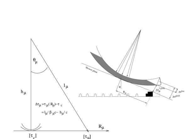
Figure 1: Sketch of a simplified relation between muon arrival time and angle of muon incidence, respectively, with the production height, neglecting multiple scattering and off-axis production ($\beta_{\mu}c$ = velocity of the muon). Additionally (right) the definitions of the arrival time quantities characterising the shape and the structure of the muon disc are indicated.

Arrival times $\tau^{1}_{\mu}<\tau^{2}_{\mu}<\tau^{3}_{\mu}$,… of the EAS muons, locally registered by timing detectors at a distance $R_{\mu}$ from the shower axis have to refer to a well defined zero-time, usually the arrival time $\tau_{c}$ of the shower core (global arrival times):

$$\Delta\tau^{n\ glob}_{\mu}=\tau^{n}_{\mu}(R_{\mu})-\tau_{c}$$

e.g.

$$\Delta\tau^{1\ glob}_{\mu}=\tau^{1}_{\mu}(R_{\mu})-\tau_{c}$$

Often there are experimental difficulties to determine the arrival time $\tau_{c}$ with sufficient experimental precision, and only ”local” times are considered. They refer to the foremost (first locally registered) muon:

$$\Delta\tau^{n\ loc}_{\mu}(R_{\mu})=\tau^{n}_{\mu}(R_{\mu})-\tau^{1}_{\mu}(R_{\mu})$$

Local arrival time distributions display the internal structure of the shower disc (characterised by various time parameters), but they do not carry information about the shape (curvature) of the front. Nevertheless studies based on simulations of the EAS development [16, 19] have shown that mass discrimination effects are just pronounced in observations of $\Delta\tau^{1\ glob}_{\mu}$.

For event-by-event observations with a fluctuating number of muons, the single relative arrival time distributions can be characterised by the mean values $\Delta\tau_{mean}$, and by various quantiles $\Delta\tau_{q}$, like the median $\Delta\tau_{0.50}$, the first quartile $\Delta\tau_{0.25}$ and the third quartile $\Delta\tau_{0.75}$. For ordered statistics of measured times $\Delta\tau_{1}\leq\Delta\tau_{2}\leq...\leq\Delta\tau_{n}$ and $k:=n\alpha+\xi,k$ integer and $\xi\in[0,1)$, the $\alpha$-quantile $\Delta\tau_{\alpha}$   $(\alpha\in(0,1))$ is the following [28, 29]:

$$\Delta\tau_{\alpha}=\left\{\begin{array}[]{ll}(\Delta\tau_{k}+\Delta\tau_{k+1})/2:&for\>\>\xi=0\\ \Delta\tau_{k}:&for\>\>\xi\in(0,1)\end{array}\right.$$

That means: in the case of large $n$, a fraction $\alpha$ of muons has arrival times less than $\Delta\tau_{\alpha}$. The mean values and dispersions (standard deviations) represent the time profile of the EAS muon component. Measurements of muon arrival time distributions and the determination of the distributions of various different time quantities have been a subject of the current investigations of the KASCADE experiment [27, 28, 30, 31, 32, 33, 34]. In these investigations the temporal EAS structure has been studied in detail in dependence on the shower size $N_{e}$, the muon number $N_{\mu}$, or the truncated muon number $N_{\mu}^{tr}$ (which is used as approximate energy identifier in KASCADE observations [41]), respectively, and from the angle of EAS incidence $\theta$. Special features arising from the observed muon multiplicity have been revealed [33]. More recently [34] using larger samples of shower events, experimentally observed with KASCADE, the sensitivity of local muon arrival time distributions and of their correlations with other EAS observable to the mass of the EAS primaries has been investigated. Methodically advanced statistical analysing techniques have been applied [42], based on Bayesian decision making for the classification of the EAS events. The procedure requires simulated distributions (processed through the detector response) as reference patterns, provided by the Monte Carlo simulation program CORSIKA [43] with a particular model of the hadronic interactions. Thus the analysis necessarily implies some model dependence. But the consistency with the invoked QGSJET model [44] could be established thanks to the measurements with varying distance $R_{\mu}$ from the shower centre and varying muon multiplicity thresholds for being accepted in the observation sample. Nevertheless, it has been also shown that the mass discrimination power of local muon arrival time distributions is rather marginal in the observed range $R_{\mu}<100$ m and primary energies $E_{0}\leq 10^{16}$ eV, and it does not significantly help for the classification.

The phenomenological features of the time structure of high energy EAS at larger distances from the shower axis have been experimentally studied with the Haverah Park [10, 11, 12, 13, 14, 15, 16] and the Akeno air shower arrays [18, 19, 20], and the results have been compared with phenomenological model predictions (scaling models and multiplicity prescriptions for the particle production in hadronic collisions). An analysis of the mass discrimination power on basis of modern models of the hadronic interactions has not yet been performed for these cases.

The recently started extension of the KASCADE detector installation: KASCADE-Grande [45] will not only provide the possibility to extend the studies of muon arrival time distributions and their correlations to larger distances $R_{\mu}$ and larger energies of the observed EAS. There is also a chance to measure global arrival times, at least for $R_{\mu}$ up to 350 m [46]. The investigations of this paper use the analysis techniques of our previous studies [29, 34] and refer mainly to the QGSJET [44], in some few comparisons also to other models. The studies are focused to explore the basic information content of muon arrival time distributions of EAS with energies up to ca. 1$\cdot 10^{18}$ eV. The analyses are completely based on data of simulated showers and consider ideal cases, i.e. neglecting the influence of the detection system. The view of interest is the discrimination of the mass of the primary particles (with adopting a particular hadronic model as generator of the reference patterns). For some observable combinations the differences in the predictions of Monte Carlo simulations using different high-energy models as generators have been scrutinised. Only marginal differences for the arrival time distributions have been found.

2 Time profiles of the EAS muon component

The present studies consider predictions of realistic and detailed Monte Carlo simulations of the EAS development initiated by cosmic ray primaries of different mass in the primary energy range up to 1$\cdot 10^{18}$ eV. The simulations have been performed by use of the program CORSIKA (version 5.64) [43], invoking in general different models for the hadronic interaction: QGSJET (version 98) [44], VENUS (version 4.125) [47] and SIBYLL (version 1.6) [48]. For the particle interactions below $E_{lab}=80$ GeV the GHEISHA [49] option is used. Earth magnetic field, observation level and particle detection thresholds have been chosen in accordance with the observation conditions of the KASCADE experiment, but without a detailed account for the detector response. The U.S. standard atmosphere (see Ref. [43]) has been adopted for the simulations. For a realistic description of the electron-photon component, instead of the NKG approximation [50] the EGS option [51] has been preferred.

Figure 2: Average global muon arrival time distributions to be observed at the distances $R_{\mu}$ to the shower core of proton and iron induced EAS at two different energies $E_{0}$ = $10^{15}$ eV (vertical incidence) and $E_{0}$ = (3.16-5.62)$\cdot 10^{17}$ eV ($0^{\circ}-30^{\circ}$) and with the muon energy detection threshold $E_{thr}$ =240 MeV (according to the threshold of the KASCADE detector array [31]).

Figure 3: ($a$) Comparison of local and global time profiles $<~{}\Delta\tau_{0.50}~{}>$ of the EAS muon component, induced by proton and Fe primaries of the energy range of (1.78-3.16)$\cdot 10^{16}$ eV, based on EAS Monte Carlo simulations using CORSIKA and the QGSJET model as generator.

Figure 3: ($b$) Local and global time profiles of different quartiles $<\Delta\tau_{q}>$ of the EAS muon component, induced by protons of the energy $E_{0}$ = (1.78-3.16)$\cdot 10^{16}$ eV from EAS Monte Carlo simulations using CORSIKA and the QGSJET model as generator.

A first set (I) of simulations comprises samples (of ca. 500 events each) of proton and Fe induced EAS of vertical incidence for various primary energy ranges, $10^{15}$ eV, (1.78-3.16)$\cdot 10^{16}$ eV and 3.16$\cdot 10^{17}$ eV, calculated with the CORSIKA version 5.62. Another set (II) of samples, calculated with a spectral index of the power-law slope of $-2.0$ for eight energy ranges ( 1$\cdot 10^{16}$ - 1.78$\cdot 10^{16}$ eV; 1.78$\cdot 10^{16}$ - 3.16$\cdot 10^{16}$ eV; 3.16$\cdot 10^{16}$ - 5.62$\cdot 10^{16}$ eV; 5.62$\cdot 10^{16}$ - 1$\cdot 10^{17}$ eV; 1$\cdot 10^{17}$ - 1.78$\cdot 10^{17}$ eV; 1.78$\cdot 10^{17}$ - 3.16$\cdot 10^{17}$ eV; 3.16$\cdot 10^{17}$ - 5.62$\cdot 10^{17}$ eV; 5.62$\cdot 10^{17}$ - 1$\cdot 10^{18}$ eV) with the CORSIKA version 5.64 and the QGSJET model, comprises smaller number of events (100 or up to only 9 for the highest energy range), distributed randomly over an angle-of-incidence range of $0^{\circ}-30^{\circ}$.

Figure 4: Fluctuations of $\rho_{\mu}^{*}$ (left) and the distribution of the reduced time $\Delta\tau_{0.50}^{*\ glob}$ (right) of proton and iron induced EAS ($E_{0}$ = (1.78-3.16)$\cdot 10^{16}$ eV) at different distances of the shower core.

For each simulated EAS event a number of EAS observable have been reconstructed: the electromagnetic shower size $N_{e}$, the muon content $N_{\mu}^{tr}$, the shower age $s$, and in particular the time parameters $\Delta\tau_{q}$ of the muon arrival time distributions and their variations with the distance $R_{\mu}$ from the shower axis. For higher primary energies and approximating the experimental conditions of KASCADE-Grande, instead of $N_{e}$ the quantity $N_{ch}$ (the total number of charged particles) is preferentially considered. Consequently we deduce also an age quantity $s_{ch}$ derived from the lateral distribution of the charged particles. As approximate energy identifier instead of $N_{\mu}^{tr}$ the quantity $\rho_{\mu}$ ($R_{\mu}$ = 600 m) with $E_{thr}=240$ MeV is introduced, which has been often considered in the past for this purpose [52, 53].

The muon arrival time distributions have been calculated for muons with an energy threshold $E_{thr}=2.4$ GeV, observed with a multiplicity $n\geq 3$ per event. The value of this energy threshold is chosen according to the muon detection threshold of the KASCADE Central Detector which is foreseen to be used for the time measurements [34]. Just for an impression average arrival time distributions for proton and iron induced EAS at two different energies and different muon energy detection thresholds are displayed in Fig. 2. The figure indicates that differences for different kinds of primaries are, if ever, obvious in the initial part of the distributions, represented by the first quartile $\Delta\tau_{0.25}$. It gives also an impression about the order of the needed time resolution (about $1.5$ ns) to reveal the differences. But generally the present paper is not focussed to the discussion of instrumental effects.

The distributions of the different quantiles $\Delta\tau_{q}$ of event-by-event observations have been shown [29, 31] to follow fairly well a phenomenological parameterisation by $\Gamma$- probability distribution functions, with parameters varying with the primary energy and the distance $R_{\mu}$.

Figure 5: Reduced local and global time profiles $<\Delta\tau_{0.50}^{*\ loc}>$ and $<\Delta\tau_{0.50}^{*\ glob}>$ of the EAS muon component induced by proton and Fe primaries of the energy range of (1.78-3.16)$\cdot 10^{16}$ eV based on Monte Carlo simulations using the QGSJET model as generator.

The following figures (Figs. 3 and 5) display the time profiles of the muon component, i.e. the variation of the mean $<\Delta\tau_{q}>$ of the time parameters and of their fluctuations (characterised by the standard deviation $\sigma_{q}$) with $R_{\mu}$. They are calculated with samples of set I and analysed for radial ranges up to 300 m (in bins $\Delta R_{\mu}$ = 10 m).

Fig. 3a compares local and global time profiles $<\Delta\tau_{0.50}>$ with respect of differences of the primary mass, while Fig. 3b displays the time profiles of different quartiles of the proton case. Obviously the local and global profiles do not exhibit pronounced differences for different primaries. The quantities $<\Delta\tau^{glob}>$ and $<\Delta\tau^{loc}>$ differ by an offset $(\Delta\tau^{glob}_{1})$ which varies with $R_{\mu}$. It has been shown that differences of $<\Delta\tau^{glob}_{1}>$ are in the order of 1 ns for different primary muons in the considered range of distances from the shower axis [54].

Since the lateral distribution of the muon component displays also some differences for different kinds of primaries, the profile of a combined quantity (”reduced time”) $\Delta\tau_{0.50}^{*}=\Delta\tau_{0.50}(R_{\mu})/\rho_{\mu}^{*}(R_{\mu})$ is of interest where $\rho_{\mu}^{*}$ represents the density of muons with energies $E_{\mu}>2.4$ GeV. This quantity is measurable with the KASCADE Central Detector and is related to the multiplicity of muons observed in the EAS event.

As an example in Fig. 4 the fluctuations of $\rho_{\mu}^{*}$ are displayed for different distances $R_{\mu}$ from the shower core, indicating an increasing separation of the distributions with increasing $R_{\mu}$. This feature is reflected in the distributions of the time quantity $\Delta\tau_{0.50}^{*\ glob}$.

Fig. 5 compares the local $<\Delta\tau_{0.50}^{*\ loc}>$ and global $<\Delta\tau_{0.50}^{*\ glob}>$ profiles. A marginally slight improvement of the discrimination of the global quantity for distances larger than 100 m is indicated. This feature gets more pronounced at higher energies. Though global quantities include the curvature of the shower disc, while local quantities display only the internal structure of the EAS. At not too large distances from the shower axis the offset between global and local profiles is nearly mass-independent.

Generally we note that differences of distributions arising from different mass primaries are in the order of nanoseconds, increasing with the distance from the shower axis. For the energies $\leq$ (1.78-3.16)$\cdot 10^{16}$ eV (set I) also some exploratory calculations, adopting the VENUS or SYBILL model, have been performed and show that the model dependence leads to differences of the distributions (within the considered $R_{\mu}$ range) in the order of 2% with no clear trend [55].

3 Correlated distributions

The concept of modern cosmic ray experiments like KASCADE or KASCADE-Grande with a multi-component detector array is to deduce the information from correlated measurements of a larger

Figure 6: The variation of the primary energy $E_{0}$ with the average of $\rho_{\mu}(600$ m), $\rho_{\mu}(300$ m), $\rho_{\mu}(180$ m) and $\rho_{\mu}(90$ m) for proton, C and Fe induced EAS.

number of observable EAS parameters for each individual event (see Ref. [56]). Particular observable quantities are the electromagnetic shower size $N_{e}$, the muon content $N_{\mu}$ (or the truncated muon number $N_{\mu}^{tr}$ in case of KASCADE) and other specific observable quantities, characterising the various EAS components. In view of the measuring possibilities of the KASCADE-Grande array the KASCADE observable $N_{e}$, $N_{\mu}$ and $N_{\mu}^{tr}$ (the latter loses also the role as approximate energy identifier for larger energies) are not accessible. For KASCADE-Grande they will be replaced by the total number of the charged particles $N_{ch}$ and a (partial) muon number, as measured with the original KASCADE detector array being embedded in the KASCADE-Grande installation. This muon number is dependent on the distance to the shower core. In the present studies, for the sake of simplicity, we represent it by $\rho_{\mu}(R_{\mu})$ i.e. the muon density (with $E_{thr}=240$ MeV) at $R_{\mu}$ and consider in particular $\rho_{\mu}(600$ m).

Figure 7: Comparison of the $N_{e}-N_{\mu}^{tr}$ correlation with the $N_{ch}-\rho_{\mu}(600$ m) correlation at different primary energies.

The variation of the muon density $\rho_{\mu}(R_{\mu})$ with the primary energy is illustrated in Fig. 6 by results of the present simulations. It is obvious that $\rho_{\mu}(600$ m) as well as the muon density at other distances (see Fig. 6) do not provide a strictly mass independent energy identifier. In addition as known for $N_{\mu}^{tr}$, there are considerable fluctuations of $\rho_{\mu}(600$ m) at fixed energies.

The current and foreseen analyses of the experiments attempt to infer from the correlations of various observable an estimate simultaneously for the energy and the mass of the primary cosmic particle inducing the EAS event. As the most powerful correlation the $N_{e}-N_{\mu}^{tr}$ correlation has been proven (see Ref. [56]). It is expected that the $N_{e}-\rho_{\mu}(R_{\mu})$ correlation will exhibit a similar discrimination power which can be defined in terms of the true classification probabilities resulting from the analysis (see section 4). The features are indicated in Fig. 7 which compares the $N_{e}-N_{\mu}^{tr}$ correlation with the $N_{ch}-\rho_{\mu}(600$ m) correlation at two different primary energies.

Correlations with additional observable EAS parameters, though of relatively small own classification power, shrink the influence of the natural EAS fluctuations and test the consistency of the analysis [57].

Figure 8: Correlation of the local quantity $\Delta\tau_{0.50}^{*\ loc}(R_{\mu})$ and of the global quantity $\Delta\tau_{0.50}^{*\ glob}(R_{\mu})$ with the $log_{10}$ $N_{e}$ for proton and iron induced showers of the energy $E_{0}=(1.00-1.78)\cdot 10^{16}$ eV in two different $R_{\mu}$ ranges.

The observation of muon arrival time distributions at particular distances $R_{\mu}$ from the shower centre is combined with the observation of the local muon density $\rho^{*}_{\mu}(R_{\mu})$ with $E_{thr}=2.4$ GeV reflected by the muon multiplicity i.e. the registered number of muons spanning the single arrival time distribution. It turned out [55] that the $\Delta\tau_{q}(R_{\mu})-\rho^{*}_{\mu}(R_{\mu})$ correlation improves the mass discrimination and can be fairly well replaced by a combined parameter $\Delta\tau_{q}^{*}(R_{\mu})=\Delta\tau_{q}(R_{\mu})/\rho^{*}_{\mu}(R_{\mu})$. This result has been already anticipated in the presentation of the EAS time profiles in section 2.

Fig. 8 displays the correlation distributions of $\Delta\tau_{0.50}^{*\ loc}(R_{\mu})$ and $\Delta\tau_{0.50}^{*\ glob}(R_{\mu})$, respectively, with the $\log_{10}N_{e}$ for proton and iron induced showers of the energy $E_{0}=(1.78-3.16)\cdot 10^{16}$ eV in two different $R_{\mu}$ ranges.

Figure 9: Correlation of $\Delta\tau_{0.50}^{*\ glob}(R_{\mu})$ with the age s and age $s_{ch}$, respectively, for proton and iron induced showers of the energy $E_{0}=(1.78-3.16)\cdot 10^{16}$ eV and $E_{0}=(1.78-3.16)\cdot 10^{17}$, respectively, in two different $R_{\mu}$ ranges.

Special interest arises from the correlation with the so-called shower age $s$. This particular EAS parameter associated with the soft EAS component is supposed to carry also some information about the longitudinal EAS development. In the cascade theory (NKG approximation) [49] $s$ is related to the actual atmospheric depth of the shower development via the lateral distribution involving the Molière radius $R_{moli\grave{e}re}$ (which is a characteristic unit of length of the scattering theory) and the ratio $E_{0}/\epsilon_{0}$ of the incident energy to the critical energy. However, the use of the age parameter resulting from the simplified handling of the electromagnetic component by the cascade theory does not describe realistically the electromagnetic component. Rather a full Monte Carlo simulation of the electromagnetic component (by use of the EGS option [51] in the CORSIKA code) calculating the total intensity distribution of the electron component and the lateral electron distribution with all fluctuations, has to be required in order to obtain results being comparable with the reality. In order to derive from lateral distributions resulting from the EGS - Monte Carlo simulation an ”age parameter” value (which is not defined within the Monte Carlo approach), the resulting lateral distribution is subsequently fitted by the NKG function $f(R/R_{moli\grave{e}re}$; $N_{e}$, $s$) in the same manner as the experimental observations are analysed ($R_{moli\grave{e}re}$ = 78 m). Thus a (lateral) ”age” is extracted [58]. In a similar way the lateral distributions of the charged particles are processed for deducing the age parameter $s_{ch}$. However it should be noted that such a procedure is considered to be only a first approximation. The lateral distribution of charged EAS particles at larger distances from the shower core deviates from the NKG function, and an improved parametrisation should be used [59]. Nevertheless Fig. 9 displays the correlation with the age parameters, defined by the NKG function. They emphasise the suggestion to exploit in analyses of experimental data correlations with the age parameters, which are obviously related to the longitudinal development and could lead to an improved discrimination of protons and iron induced EAS.

In the following section we base such qualitative statements deduced from the inspection of the distributions (shown as examples in Figs. 8 and 9) on quantitative results of statistical analyses of multivariate distributions, considering also the more complicated case of three mass classes (protons: H, carbon: C, iron: Fe).

4 Non-parametric analyses of the sensitivity to the primary mass

Non-parametric statistical methods are most efficient and unbiased tools for the analysis of multidimensional observable-distributions in order to associate single observed events to different classes (say to different masses of the EAS primaries) by comparing the considered events with the model distributions without using any pre-chosen parameterisation. The methods of decision making and the application to cosmic ray data analyses are generally described in Refs.[42, 56]. They have been outlined for studies of muon arrival time distributions in Refs.[27, 29]. The procedures take into account the effects of the natural EAS fluctuations in a quite natural way and are able to specify the uncertainties, by an estimate of the true-classification and misclassification probabilities. The classification probabilities are determined by the extent to which the likelihood functions of the single classes, derived from the simulations, are overlapping. Basically the results of such pattern recognition methods, using trained neural networks or Bayes decision rules, are dependent from the particular hadronic interaction model generating the reference pattern for the data to be studied. In the present analysis of the sensitivity of various correlation distributions, prepared from Monte Carlo simulations, the so-called one-leave-out test (see Ref. [42]) is applied, which determines the probability that a multidimensional event, taken from the considered (simulated) distribution, will be correctly (”true”) or incorrectly (”false”) classified by the procedure.

Figure 10: Comparison of the classification probabilities deduced from the $\Delta\tau_{0.50}^{\ glob}(R_{\mu})-N_{e}$, the $\Delta\tau_{0.50}^{*\ glob}(R_{\mu})-N_{e}$ and the $\Delta\tau_{0.50}^{\ glob}(R_{\mu})-\rho_{\mu}^{*}(R_{\mu})-N_{e}$ correlations at the incident energy of (1.00-1.78)$\cdot 10^{16}$ eV at $R_{\mu}$ = 175-185 m (left). Similarly the classification probabilities deduced from the $\Delta\tau_{0.50}^{\ glob}(R_{\mu})-N_{ch}$, the $\Delta\tau_{0.50}^{*\ glob}(R_{\mu})-N_{ch}$ and the $\Delta\tau_{0.50}^{\ glob}(R_{\mu})-\rho_{\mu}^{*}(R_{\mu})-N_{ch}$ correlations at the incident energy of (1.00-1.78)$\cdot 10^{17}$ eV are shown (right). The lines are drawn for guiding the eyes.

Figure 11: The influence of the global time parameter $\Delta\tau_{0.50}^{\ glob}(R_{\mu})$ and the accompanying $\rho_{\mu}^{*}(R_{\mu})$ on the true and false - classifications of the $N_{e}-N_{\mu}^{tr}$ correlation shown for the primary energy (1.00-1.78)$\cdot 10^{16}$ eV at $R_{\mu}$ = 175-185 m. Similarly the influence on the true and false - classifications of the $N_{ch}-\rho_{\mu}(R_{\mu})$ correlation is shown for the primary energy (1.00-1.78)$\cdot 10^{17}$ eV (right). For the explanation of the symbols see Fig. 10.

Figure 12: ($a$) The influence of the global time parameter $\Delta\tau_{0.50}^{*\ glob}(R_{\mu})$ on the true and false - classifications of the $N_{e}-N_{\mu}^{tr}$ correlation shown for two distances $R_{\mu}$ for the primary energy range (1.0-1.78)$\cdot 10^{16}$ eV. For the explanation of the symbols see Fig. 10.

Figure 12: ($b$) The influence of the global time parameter $\Delta\tau_{0.50}^{*\ glob}(R_{\mu})$ on the true and false - classifications of the $N_{ch}-\rho_{\mu}(R_{\mu})$ correlation shown for two distances $R_{\mu}$ and for the primary energy range (1.0-1.78)$\cdot 10^{17}$ eV. For the explanation of the symbols see Fig. 10.

The following figures present the classification ($H\rightarrow H$; $C\rightarrow C$; $Fe\rightarrow Fe$) and misclassification ($H\rightarrow C,Fe$; $C\rightarrow H,Fe$; $Fe\rightarrow H,C$) probabilities for various correlations of different EAS observable. The discrimination power may be quantified by the “Bayes risk” defined as

$$R=\>\frac{1}{M_{i}}\>\>\sum_{j=1}^{M_{i}}\varepsilon(x_{j})$$

where

$$\varepsilon(x_{j})=\left\{\begin{array}[]{ll}0&\>\>for\>\>true\>\>classification\\ 1&\>\>otherwise\end{array}\right.$$

of the event $x_{j}$ of the sample $M_{i}$. When considering the results based on simulations, one should keep in mind that the primary energy $E_{0}$ is a-priori known, while in the real cases $E_{0}$ has to be simultaneously estimated from the data, in particular from the $N_{e}-N_{\mu}^{tr}$ correlation. Within a limited energy range $N_{\mu}^{tr}$ can be used as approximate energy identifier. From this reason correlations of $N_{\mu}^{tr}$ with time observable are not specially scrutinised.

Even with the primary energy given, the fluctuations of $N_{e}$ and $N_{ch}$ or of the correlations $\Delta\tau_{0.50}^{\ glob}(R_{\mu})-N_{e}$ and $\Delta\tau_{0.50}^{\ glob}(R_{\mu})-N_{ch}$ are so large, that the true classification probability remains modest. Fig. 10 confirms the approximate equivalence of the parameter $\Delta\tau_{0.50}^{*}(R_{\mu})$ with the $\Delta\tau_{0.50}(R_{\mu})-\rho_{\mu}^{*}(R_{\mu})$ correlation, though the $\Delta\tau_{0.50}(R_{\mu})-\rho_{\mu}^{*}(R_{\mu})$ correlation appears obviously preferable in view of the mass classification. It is obvious that the quantity $\rho_{\mu}^{*}(R_{\mu})$ (simultaneously observed with multiplicity in arrival time measurements of KASCADE (see Ref. [34])) leads to a considerable stabilisation of the discrimination effect. Especially when observables (like $N_{e}$ and $\Delta\tau_{q}$) of comparatively weak discrimination power are correlated. We conclude that the time quantities $\Delta\tau_{q}$ should be preferentially introduced in combination with $\rho_{\mu}^{*}(R_{\mu})$, if ever experimentally possible.

The effect of global muon arrival time distributions, represented by $\Delta\tau_{0.50}^{\ glob}(R_{\mu})$ is quantified by the classification probabilities given in Fig. 11. When the detector installation is able to measure the $N_{e}-N_{\mu}^{tr}$ correlation, adding $\rho_{\mu}^{*}(R_{\mu})$ and $\Delta\tau_{0.50}^{\ glob}(R_{\mu})$ has only a minor discrimination effect, even at larger distances from the shower core. This is in contrast to the case, when only $N_{ch}$ and a partial muon number (in our analysis approximated by $\rho_{\mu}(R_{\mu})$) are experimentally accessible. At larger distances, especially for the higher primary energies, the correlation of muon arrival times has a clear effect of improving the mass discrimination. It is interesting to note that this result holds also approximately for local time parameters.

Fig. 12a displays the $R_{\mu}$-dependence of the influence of the global time parameter $\Delta\tau_{0.50}^{*\ glob}(R_{\mu})$ on the true and false - classifications of the $N_{e}-N_{\mu}^{tr}$ correlation for the primary energy range (1.0-1.78)$\cdot 10^{16}$ eV. At a first glance surprisingly, there is no significant tendency with increasing $R_{\mu}$. This feature can be understood with the above arguments of the minor contribution of the muon arrival time parameter when the ($R_{\mu}$ independent) $N_{e}-N_{\mu}^{tr}$ correlation can be determined.

However, due to the generally weaker discrimination power of the $N_{ch}-\rho_{\mu}(R_{\mu})$ correlation the influence of $\Delta\tau_{0.50}^{\ glob}(R_{\mu})$ appears significant in this case (Fig. 12b), though also not significantly varying with the distance. For example the improvement in terms of the Bayes risk for the case of $E_{0}=10^{16}eV$ is only 2%-3% while in the case of $E_{0}=10^{17}eV$ it is 14%-15%, i.e. not negligible.

Figure 13: Comparison of the influence of different quartiles of global arrival time distributions on the $N_{ch}-\rho_{\mu}$ correlation. For the explanation of the symbols see Fig. 10.

As indicated in Fig. 13 differences in the discrimination effects of different quartiles $\Delta\tau_{q}$ are hardly obvious and may be obscured by the inherent fluctuations. Studies of the classification and misclassification probabilities of EAS observable correlations including the age parameters show a non-negligible sensitivity of these EAS parameters. However, when alone correlated with $N_{e}(N_{ch})$ such a correlation (say $N_{e}-s$) proves to be a very uncertain and instable discriminator due to the fact that fluctuations of both related observables do obviously corroborate. Adding an observable of another EAS component stabilises the classification result.

From the classification and misclassification studies following features and tendencies can be recognised:

• The reduced time parameter $\Delta\tau_{q}^{*}=\Delta\tau_{q}(R_{\mu})/\rho_{\mu}^{*}(R_{\mu})$ (where $\rho_{\mu}^{*}$ represents the density of muons with energies $E_{\mu}>2.4$ GeV) absorbs partially the $\Delta\tau_{q}(R_{\mu})-\rho_{\mu}^{*}(R_{\mu})$ correlation and enhances the mass classification sensitivity.

• The most important features are condensed in Figs. 11 and 12, revealing a significant contribution of the muon arrival time information when correlated with the EAS observable $N_{ch}$ and $\rho_{\mu}(R_{\mu})$, experimentally accessible by the foreseen layout of KASCADE-Grande.

• The shower age parameters $s$ and $s_{ch}$ (which have been scrutinised as additional parameters) have modest, but non-negligible effects for the mass discrimination.

• Correlations of largely fluctuating quantities, resulting from related observations (like $N_{e}$ and $s$, e.g.), lead to a bad classification with large uncertainties, but adding the correlation with an observable from another EAS component (like $\Delta\tau_{q}^{*}$), even also fluctuating, induces an considerable improvement.

As already mentioned - as additional calculations show - the model dependence of the results of the classification probabilities is rather marginal. However, it should be remarked, this feature could be in detail different for different EAS parameter correlations and is also not yet explored for higher energy ranges.

5 The efficiency of the observation conditions and the energy and mass dependence

Figure 14: The probabilities to register EAS events from proton and Fe induced EAS of different primary energies under the observation conditions ($E_{thr}$ =2.4 GeV, $n_{thr}$, $R_{\mu}$) with a $10\cdot 10$ m² ideal detector. The variation with $R_{\mu}$ and with the multiplicity threshold $n_{thr}$ is displayed.

By the observations of muon arrival time distributions special samples of all observed EAS events are selected due to the particular observation conditions, especially by the energy threshold $E_{thr}$ (= 2.4 GeV in the actual case) of the detected muons and the multiplicity threshold $n_{thr}$, i.e. the number of muons necessary to define an event with an observable arrival time distribution. Thus the event selections are affected by the lateral distribution and the energy spectrum of EAS muon. Consequently the probability being accepted in the event sample depends on the observation distance $R_{\mu}$, on $n_{thr}$ and on the mass of the EAS primary. As discussed in Ref. [34] this feature implies in experimental observations of EAS samples efficiency corrections [60] and enables consistency tests by varying $R_{\mu}$ and $n_{thr}$ in the measurements.

Fig. 14 displays the results of calculations of the efficiency to register an EAS event under the specified conditions of muon arrival time measurements.

The efficiency depends strongly on $R_{\mu}$ and $n_{thr}$ at lower primary energies ($10^{15}$ eV) in a qualitatively understandable way. The dependence gets weaker at higher primary energies. In general the dependence and the variation with $R_{\mu}$ and $n_{thr}$ are different for different primary masses.

6 Conclusions

In the present paper based on realistic EAS Monte Carlo simulations the role of muon arrival time distributions has been scrutinised in view of correlations with the main EAS observables to be measured with the KASCADE-Grande layout for the discrimination of the primary mass at higher primary energies. The main observables for that purpose are the total number of the charged particles $N_{ch}$ and a part of the EAS muon intensity $N_{\mu}^{part}(R_{\mu})$ registered with the KASCADE array, embedded in KASCADE-Grande. The partial muon number $N_{\mu}^{part}(R_{\mu})$ is dependent from the location of the EAS centre. For the present simulation studies it has been replaced by the density $\rho_{\mu}(R_{\mu})$ ($E_{\mu}>240$ MeV). In summary, the analyses of the classification and misclassification probabilities, determined with non-parametric statistical techniques give evidence that the information from muon arrival time distributions has a potential for improving the mass discrimination. This conclusion, being in contrast to findings at lower energies, holds for global time quantities as well as for the local ones. Actually the EAS profiles of the two different types of time parameters differ by an offset being only marginally dependent from the mass. This is due to an increasing “flatness” of the $<\Delta\tau_{1}>$ profile with increasing primary energy, and differences are moved to larger distances out of experimental reach. This feature is important with respect to the experimental difficulties to define $\tau_{c}$ and to measure global time quantities. Obviously in the considered $R_{\mu}$ range the local times provide most of the accessible information.

The measuring techniques of muon arrival time distributions with the Central Detector of KASCADE imply the simultaneous determination of the multiplicity $n$ of muons spanning the arrival distributions. This multiplicity is related to the density $\rho_{\mu}^{*}(R_{\mu})$ of the higher energy muons detected with the facilities of the Central Detector. The quantity $\rho_{\mu}^{*}(R_{\mu})$ (or the number of muons experimentally detected with the timing facility), when correlated with timing measurements (or used as $\Delta\tau_{q}^{*}=\Delta\tau_{q}(R_{\mu}/\rho_{\mu}^{*}(R_{\mu})$) plays an important role in improving the effects of the arrival time observations.

Additionally (as outlined in Ref.[34]) as consequence of the specific observation conditions muon arrival time observations establish a selected subset of all showers, and the determination of the mass composition needs a corresponding correction [60]. Thus the results inferred with a variation of the multiplicity threshold $n_{thr}$ and of the observation distance $R_{\mu}$ provide a consistency test for the model used for the non-parametric analyses of the observed EAS.

It should be noted that the present results refer to ideal cases since any detector response functions, detector efficiencies and limitations of the statistical accuracies due to limited detector sizes have been ignored. Additionally the necessarily limited number of simulated EAS implies a limit on the reasonable number of observables used in a single analyses.

References

References

- [1] P. Bassi, G. Clark and B. Rossi, Phys. Rev. 92 (1953) 441
- [2] J. V. Jelley and W. J. Whitehouse, Proc. Phys. Soc. (London) A66 (1953) 454
- [3] J. Linsley, L. Scarsi, B. Rossi, Phys. Rev. Lett. 6 (1961) 485; Phys. Rev. 128 (1962) 2384
- [4] C. P. Woidneck and E. Böhm, J. Phys. A: Math.Gen. 8 (1975) 997
- [5] H. E. Dixon and K. E. Turver, Proc. R. Soc. A 339 (1974)171
- [6] J. Lapikens, J. Phys. A: Math. Gen. 8 (1975) 838
- [7] P. K. F. Grieder, Nuovo Cimento 7 (1977) 1
- [8] J. Linsley and A. A. Watson, Phys. Rev. Lett. 46 (1981) 459
- [9] J. Linsley, J. Phys. G: Nucl. Part. Phys. 12 (1986) 51
- [10] A. J. Baxter, A. A.Watson and J. G. Wilson, Canadian J. Phys. 46 (1968) S9
- [11] P. R. Blake et al., J. Phys. G: Nucl. Phys. 8 (1982) 1605
- [12] M. L. Armitage, P. R. Blake and W. F. Nash, J. Phys. A: Math. Gen. 8 (1975) 1005
- [13] A. A. Watson and J. G. Wilson, J. Phys. A: Math. Gen. 7 (1976) 1199
- [14] R. Walker and A.A. Watson, J. Phys. G: Nucl. Phys. 7 (1981) 129, ibid 8 (1982) 1131
- [15] M. L. Armitage et al., J. Phys. G: Nucl. Phys. 13 (1987) 707
- [16] P. R. Blake et al., J. Phys G: Nucl. Part. Phys 16 (1990) 755
- [17] E. J. deVilliers et al., J. Phys. G: Nucl. Phys. 12 (1986) 547
- [18] N. Inoue et al., J. Phys. G: Nucl. Phys. 11 (1985) 657, ibid 11 (1985) 669
- [19] F. Kakimoto et al., J. Phys. G: Nucl. Phys. 9 (1983) 339, ibid 16 (1986) 151
- [20] M. Teshima et al., J. Phys. G: Nucl. Phys. 12 (1986) 1097
- [21] G. B. Khristiansen et al., Proc. 21th ICRC, Adelaide, Australia, 1990, vol. 9, p. 150
- [22] G. Agnetta et al., Astropart. Phys. 6 (1997) 301
- [23] M. Ambrosio et al., Astropart. Phys. 7 (1997) 329
- [24] M. Ambrosio et al., J. Phys. G: Nucl. Part. Phys. 23 (1997) 219
- [25] M. Ambrosio et al., Astropart. Phys. 11 (1999) 427
- [26] G. Battistoni et al., Astropart. Phys. 9 (1998) 277
- [27] H. Rebel et al., J. Phys. G: Nucl. Part. Phys. 21 (1995) 451; H. Rebel, Proceedings XV Cracow Summer School of Cosmology The Cosmic Ray Mass Composition, Lodz, Poland, 15-19 July, 1996, ed. W. Tkaczyk, p. 91
- [28] M. Föller, U. Raidt et al., KASCADE Collaboration, Proc. 25th ICRC, Durban, South Africa, 1997, vol. 6, p. 149
- [29] I. M. Brancus et al., Astropart. Phys. 7 (1997) 343
- [30] I. M. Brancus et al., KASCADE Collaboration: Proc. 26th ICRC, Salt Lake City, USA, 1999, eds. D. Kieda et al., vol. 1, p. 345
- [31] T. Antoni et al., KASCADE Collaboration, Astropart. Phys. 15 (2001) 149
- [32] A.F. Badea et al., Astropart. Phys. 15 (2001) 19
- [33] R. Haeusler et al., Astropart. Phys. 17 (2002) 421
- [34] T. Antoni et al., KASCADE Collaboration, The information from muon arrival time distributions of high energy EAS measured with the KASCADE experiment, Astropart. Phys. (2002), in press
- [35] J. A. Goodman et al., Phys. Rev. Lett. 42 (1979) 854; Phys. Rev. D 26 (1982) 1043
- [36] T. V. Danilova et al., J. Phys. G: Nucl. Part. Phys. 20 (1995) 961
- [37] J. Hörandel et al., KASCADE Collaboration, Contr. XII ISVHECRI 2002, Geneva, Switzerland, to be published in Nucl. Phys. B
- [38] K. Bernlöhr, Astropart. Phys. 5 (1996) 139
- [39] P. Doll et al., Nucl. Instr. and Meth. A 488 (2002) 517; J. Zabierowski et al., KASCADE Collaboration, Proc. 27th ICRC Hamburg, Germany, 2001, vol. 6, p. 810
- [40] J. Linsley, Nuovo Cimento 15C (1992) 743
- [41] J. H. Weber et al., KASCADE Collaboration, Proc. 25th ICRC Durban, South Africa, 1997, vol. 2, p. 810
- [42] A. A. Chilingarian, Comp. Phys. Comm. 54 (1989) 381; A. A. Chilingarian and G. Z. Zazian, Nuovo Cim.14 (1991) 355; ANI reference manual, 1999 unpublished
- [43] D. Heck et al., FZKA-Report 6019, Forschungszentrum Karlsruhe (1998)
- [44] N. N. Kalmykov, S. Ostapchenko and A. I. Pavlov, Nucl. Phys. B. (Proc. Suppl.) 52B (1997) 17
- [45] M. Bertaina et al., KASCADE-Grande Collaboration, Proc. 27th ICRC Hamburg, Germany, 2001, vol. 2, p. 792
- [46] H. Bozdog, H. J. Mathes, private communication
- [47] K. Werner, Phys. Rep. 232 (1993) 87
- [48] R. S. Fletcher et al., Phys. Rev. D 50 (1994) 5710
- [49] H. Fesefeldt, PITHA-85/02, RWTH Aachen (1985)
- [50] K. Kamata and J. Nishimura, Prog. Theo. Phys. Suppl. 6 (1958) 93; J. Nishimura, Handbuch der Physik 46 (1967) 1
- [51] W. R. Nelson, H. Hirayama and D. W. O. Rogers, Report SLAC 265, Stanford Linear Accelerator Center (1985)
- [52] D. M. Edge et al., J. Phys. A: Math. Nucl. Gen. 6 (1973) 1612
- [53] H. Y. Dai et al., J. Phys. G: Nucl. Part. Phys. 14 (1988) 793
- [54] R. Haeusler, FZKA-Report 6520, Forschungszentrum Karlsruhe (2000)
- [55] I. M. Brancus, Internal Report KASCADE-09/2000-02, Forschungszentrum Karlsruhe (2000)
- [56] H. Rebel, Progr. Part. Nucl. Phys. 46 (2001) 109
- [57] T. Antoni et al., KASCADE Collaboration, Astropart. Phys. 16 (2002) 245
- [58] T. Antoni et al., KASCADE Collaboration, Astropart. Phys. 14 (2001) 245
- [59] R. Ulrich, FZKA-Report 6787, Forschungszentrum Karlsruhe (2002)
- [60] A. F. Badea, FZKA-Report 6579, Forschungszentrum Karlsruhe (2001)