Color Variability of AGNs

Abstract

Optical spectral variability of quasars and BL Lac Objects is compared by means of the spectral variability parameter $\beta$ (Trevese & Vagnetti, 2002). Both kinds of objects change their spectral slopes $\alpha$, becoming bluer when brighter, but BL Lac Objects have smaller $\beta$ values and are clearly separated from quasars in the $\alpha-\beta$ plane. Models accounting for the origin of the variability are discussed for both classes of objects.

1 Introduction

Variability of the spectral energy distribution (SED) of Active Galactic Nuclei (AGNs) is a powerful tool to investigate the role of the main emission processes in different AGN classes, and the origin of their variations. The most common behavior in the optical band is that AGNs become bluer, i.e. their spectrum becomes harder, when brighter. This has been shown for individual Quasi Stellar Objects (QSOs) and Seyferts (Cutri et al., 1985; Edelson, Krolik & Pike, 1990; Kinney et al., 1991; Paltani & Courvoisier, 1994) and for one complete sample, i.e. for the 42 PG QSOs monitored by Giveon et al. (1999) in B and R for 7 years. Evidence based on two epochs has been found also for the faint QSO sample in the SA 57 (Trevese, Kron, & Bunone, 2001). The same trend is apparently shared by BL Lac Objects, as shown by D’Amicis et al. (2002), who present 5-year long B, V, R, I light curves for eight objects. A quantitative estimate of color variability is necessary to compare the observational data with emission models and to compare different AGN classes. In a previous paper (Trevese & Vagnetti, 2002), we introduced the spectral variability parameter $\beta\equiv\Delta\alpha/\Delta\log f_{\nu}$, $f_{\nu}$ being the specific flux and $\alpha\equiv\partial\log f_{\nu}/\partial\log\nu$ the spectral slope. From the average $\alpha$ and $\beta$ values, it was possible to derive constraints on the variability mechanisms. The spectral variability parameter was then estimated (Vagnetti, Trevese & Nesci, 2002) for the BL Lac Objects of D’Amicis et al. (2002). Observations and models can be compared in the $\alpha-\beta$ plane, which is reported in Fig. 1 for both the PG QSOs and the BL Lac Objects.

2 Quasars

Various models have been compared with the spectral variability of PG QSOs (Trevese & Vagnetti, 2002) and are shown in Fig. 1.

(i) The dot-dashed line represents the spectral variability due to small temperature changes for a sequence of black bodies with different temperatures (increasing from left to right).

(ii) We evaluate the effect of the host galaxy through numerical simulations based on templates of the QSO and host galaxy SEDs, derived from the atlas of normal QSO continuum spectra (Elvis et al., 1994). We added to the fixed host galaxy template SED the average QSO spectrum with a relative weight measured by the parameter $\eta\equiv\log({L_{H}^{Q}}/{L_{H}^{g}})$, where ${L_{H}^{Q}}$ and ${L_{H}^{g}}$ are the total $H$ band luminosities of the QSO and the host galaxy respectively. Variability is represented by small changes $\Delta\eta$, around each $\eta$ value, with an amplitude corresponding to a r.m.s. variability $\sigma_{B}=0.16$ mag in the blue band. The result is shown in Fig. 1 for $-3<\eta<3$ and for $z=0$, represented by a thin, continuous line, and clearly shows that the effect of the host galaxy is not sufficient to account for the observed changes of the spectral slope.

(iii) We considered the accretion disk model of Siemiginowska et al. (1995), corresponding to a Kerr metric and modified black body SED, which depend on the black hole mass $M$, the accretion rate $\dot{M}$ and the inclination $\theta$. A change of $\dot{m}\equiv\dot{M}c^{2}/L_{E}$ ($L_{E}$ being the Eddington luminosity) produces a variation of both luminosity and the SED shape. The result is represented in Fig. 1 by a thick, dashed curve, for $\dot{m}$ varying between 0.1 and 0.3, and for $\theta=0$ (face on disk). The spectral variations are clearly smaller, on average, than the observed ones. This means that a transition e.g. from a lower to a higher $\dot{M}$ regime implies a larger luminosity change for a given slope variation, respect to what is observed.

(iv) Transient phenomena, like hot spots produced on the accretion disk by instability phenomena (Kawaguchi et al., 1998), instead of a transition to a new equilibrium state, may better explain the relatively large changes of the local spectral slope. We use a simple model based on the addition of a black body flare to the disk SED, represented by the average QSO SED of Elvis et al. (1994). The result is shown in Fig. 1 by the large filled squares, corresponding to hot spots with $T\approx 10^{5}$ K (upper), and $T\approx 6\cdot 10^{4}$ K (lower).

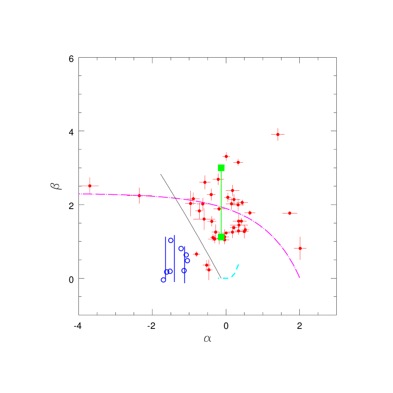
Figure 1: The spectral variability parameter $\beta$ versus the average spectral slope $\alpha$ for two samples of QSOs (dots) and BL Lac Objects (open circles). QSOs & BL Lac Objects appear clearly separated. Model predictions for both classes of objects are discussed in the text: black body (dot-dashed line), effect of the host galaxy (thin line), change of accretion rate (thick dashed line), hot spots (large filled squares), synchrotron emission for BL Lac Objects (vertical lines).

3 BL Lac Objects

The continuum spectral energy distribution of blazars from radio frequencies to X and $\gamma$-rays can be explained by a synchrotron emission plus inverse Compton scattering (Sikora, Begelman, & Rees, 1994). Variability can be produced by an intermittent channeling into the jet of the energy produced by the central engine. Spada et al. (2001) have considered a detailed model where crossing of different shells of material, ejected with different velocities, produce shocks which heat the electrons responsible for the synchrotron emission. The resulting spectra are compared with multi-band, multi-epoch observations of 3C 279 from radio to $\gamma$ frequencies, showing a good agreement. In the case of the eight objects of our sample, B, V, R, I bands are sampling variability of the synchrotron component. This component can be roughly described by a broken power law characterized by the break (or peak in $\nu L_{\nu}$) frequency $\nu_{p}$ and the asymptotic spectral slopes $\alpha_{1}$ end $\alpha_{2}$ at low and high frequency respectively, $\alpha_{1}>-1$, $\alpha_{2}<-1$ (Tavecchio, Maraschi & Ghisellini, 1998). We adopt (Vagnetti, Trevese & Nesci, 2002) the equivalent representation

$$L_{\nu}={2L_{p}\over(\frac{\nu}{\nu_{p}})^{-\alpha_{1}}+(\frac{\nu}{\nu_{p}})^{-\alpha_{2}}}\equiv$$

$$\equiv L_{p}\cdot H(\nu;\alpha_{1},\alpha_{2},\nu_{p})$$ (1)

for a stationary component of the SED and we add to it a second (variable) component with the same analytical form but different peak frequency $\nu_{p^{\prime}}$ and amplitude $L_{p^{\prime}}$ to produce spectral changes:

$$L_{\nu}=L_{p}\cdot H(\nu;\alpha_{1},\alpha_{2},\nu_{p})+$$

$$+L_{p^{\prime}}\cdot H(\nu;\alpha_{1},\alpha_{2},\nu_{p^{\prime}})$$ (2)

The addition of the second component mimics the behavior of the synchrotron emission of model spectra when shell crossing occurs, producing an increment of emission with $\nu_{p^{\prime}}>\nu_{p}$, due to newly accelerated electrons. With such a representation we can compute $\alpha$ and $\beta$ as a function of $\nu_{p^{\prime}}/\nu_{p}$, for different values of $\nu_{p}$ and given values of $\alpha_{1}$, $\alpha_{2}$ and $L_{p^{\prime}}/L_{p}$. We adopt typical values of the asymptotic slopes (Tavecchio, Maraschi & Ghisellini, 1998) $\alpha_{1}=-0.5$, $\alpha_{2}=-1.75$, we assigned to $\nu_{p}$ different values in the range $10^{14}-10^{15}$, we made $\nu_{p^{\prime}}/\nu_{p}$ vary in the range $\approx 1-10$ and we adopted $L_{p^{\prime}}/L_{p}$ corresponding to a magnitude change of 1 mag r.m.s. The results are shown in Fig. 1, where for $\alpha$ we use the slope of the stationary component. The three vertical lines are computed for $\log\nu_{p}=14,14.5,14.8$ from left to right respectively. The computed lines fall naturally in the region occupied by the data, namely it is possible to account for the position of the objects in the $\alpha-\beta$ plane with typical values of $\alpha_{1}$, $\alpha_{2}$, $\nu_{p^{\prime}}/\nu_{p}$ and $\nu_{p}$, corresponding to the overal SED of the objects considered (see Fossati et al., 1998).

4 Conclusions

We show that the spectral variability parameter $\beta$ is a powerful tool to discriminate between different models of the variability of AGNs. Hot spots on the disk, likely produced by local instabilities, are able to account for the observed spectral variability of QSOs.

We show that BL Lacs clearly differ from QSOs in their $\alpha,\beta$ distribution. A simple model representing the variability of a synchrotron component can account for the observed $\alpha$ and $\beta$ values.

In the framework of wide field variability studies, we stress that observations in at least two photometric bands, repeated on the same field at many epochs, would allow a detailed test of variability models, extending our knowledge of the emission processes in AGNs.

References

- Cutri et al. (1985) Cutri, R. M., Wisniewski, W. Z., Rieke, G. H., & Lebofski, H. J. 1985, ApJ, 296, 423
- D’Amicis et al. (2002) D’Amicis, R., Nesci, R., Massaro, E., Maesano, M., Montagni, F., D’Alessio, F., 2002, pasau, 19, 111
- Edelson, Krolik & Pike (1990) Edelson, R.A., Krolik, J. H.,& Pike, G. F. 1990, ApJ, 359, 86
- Elvis et al. (1994) Elvis, M., Wilkes, B. J., McDowell, J. C., Green, R. F., Bechtold, J., Willner, S. P., Oey, M. S., Polomski, E., Cutri, R., 1994, ApJS, 95, 1
- Fossati et al. (1998) Fossati, G, Maraschi, L., Celotti, A., Comastri, A., & Ghisellini, G., 1998, MNRAS, 299,433
- Giveon et al. (1999) Giveon, U., Maoz, D., Kaspi, S., Netzer, H., & Smith P. S. 1999, MNRAS, 306, 637
- Kawaguchi et al. (1998) Kawaguchi, T., Mineshige, S., Umemura, M., & Turner, E. L. 1998, ApJ, 504, 671
- Kinney et al. (1991) Kinney, A. L., Bohlin, R.C., Blades, J. C., & York, D. G. 1991, ApJS, 75, 645
- Paltani & Courvoisier (1994) Paltani, S., & Courvoisier, T. J.-L. 1994, A&A, 291, 74
- Siemiginowska et al. (1995) Siemiginowska, A. Kuhn, O., Elvis, M., Fiore, F., McDowell, J., & Wilkes, B., 1995, ApJ, 454, 77
- Sikora, Begelman, & Rees (1994) Sikora, M., Begelman, M. & Rees, M.J., 1994, ApJ, 421, 153
- Spada et al. (2001) Spada, M., Ghisellini, G., Lazzati, D., & Celotti, A., 2001, MNRAS, 325, 1559
- Tavecchio, Maraschi & Ghisellini (1998) Tavecchio, F., Maraschi, L., & Ghisellini, G., 1998, ApJ, 509, 608
- Trevese, Kron, & Bunone (2001) Trevese, D., Kron, R. G., & Bunone A., 2001, ApJ, 551, 103
- Trevese & Vagnetti (2002) Trevese, D., & Vagnetti, 2002, ApJ, 564, 624
- Vagnetti, Trevese & Nesci (2002) Vagnetti, F., Trevese, D., & Nesci, R., 2002, in preparation