$H_{2}^{+}$ molecular ion in a strong magnetic field: ground state

Abstract

A detailed quantitative analysis of the system $(ppe)$ placed in magnetic field ranging from $0-4.414\times 10^{13}\,G$ is presented. The present study is focused on the question of the existence of the molecular ion $H_{2}^{+}$ in a magnetic field. As a tool, a variational method with an optimization of the form of the vector potential (optimal gauge fixing) is used. It is shown that in the domain of applicability of the non-relativistic approximation the system $(ppe)$ in the Born-Oppenheimer approximation has a well-pronounced minimum in the total energy at a finite interproton distance for $B\lesssim 10^{11}\,G$, thus manifesting the existence of $H_{2}^{+}$. For $B\gtrsim 10^{11}\,G$ and large inclinations (of the molecular axis with respect to the magnetic line) the minimum disappears and hence the molecular ion $H_{2}^{+}$ does not exist. It is shown that the most stable configuration of $H_{2}^{+}$ always corresponds to protons situated along the magnetic line. With magnetic field growth the ion $H_{2}^{+}$ becomes more and more tightly bound and compact, and the electronic distribution evolves from a two-peak to a one-peak pattern. The domain of inclinations where the $H_{2}^{+}$ ion exists reduces with magnetic field increase and finally becomes $0^{o}-25^{o}$ at $B=4.414\times 10^{13}\,G$. Phase transition type behavior of variational parameters for some interproton distances related to the beginning of the chemical reaction $H_{2}^{+}\leftrightarrow H+p$ is found.

I Introduction

Many years have passed since the moment when theoretical qualitative arguments were given that show that in the presence of a strong magnetic field the physics of atoms and molecules exhibits a wealth of new, unexpected phenomena even for the simplest systems Kadomtsev:1971 ; Ruderman:1971 . In particular, a chance that unusual chemical compounds may be formed which do not exist without magnetic field was mentioned. In practice, the atmosphere of neutron stars, which is characterized by the presence of enormous magnetic fields $10^{12}-10^{13}\,G$, as well as other astronomical objects carrying large magnetic fields ($>10^{8}\,G$) provide a valuable paradigm where this physics could be realized. Recently, the experimental data collected by the Chandra X-ray observatory revealed certain irregularities in the spectrum of an isolated neutron star 1E1207.4-5209. These irregularities can be interpreted as absorption features at $\sim 0.7\,$ KeV and $\sim 1.4\,$ KeV of possible atomic or molecular nature Sandal:2002 .

One of the first general features observed in standard atomic and molecular systems placed in a strong magnetic field is an increase of both total and binding energies, accompanied by a drastic shrinking of the electron localization length in both the longitudinal and transverse directions. Naturally, this leads to a decrease of the equilibrium distance with magnetic field growth. This behavior can be considered to be a consequence of the fact that for large magnetic fields the electron cloud takes a needle-like form extended along the magnetic field direction and the system becomes effectively quasi-one-dimensional Ruderman:1971 . It is obvious that the phenomenon of quasi-one-dimensionality enhances the stability of standard atomic and molecular systems from the electrostatic point of view. In particular, molecules become elongated along the magnetic line forming a type of linear molecular polymer (for details see the review articles Garstang:1977 ; Lai:2001 ). It also hints at the occurrence of exotic atomic and molecular systems which do not exist in the absence of a magnetic field. Motivated by these simple observations it was shown in Refs.Turbiner:1999 ; Lopez-Tur:2000 that three and even four protons can be bound by one electron. This shows that exotic one-electron molecular systems $H_{3}^{2+}$ and $H_{4}^{3+}$ can exist in sufficiently strong magnetic fields in the form of linear polymers. However, the situation becomes much less clear (and also much less studied) when the nuclei are not aligned with the magnetic field direction, and thus in general do not form a linear system. Obviously, such a study would be important for understanding the kinetics of a gas of molecules in the presence of a strong magnetic field. As a first step towards such a study, even the simplest molecules in different spatial configurations deserve attention. Recently, a certain spatial configuration of $H_{3}^{2+}$ was studied in detail Lopez-Tur:2002 . It was shown that in the range of magnetic fields $10^{8}<B<10^{11}\,G$ the system $(pppe)$, with the protons forming an equilateral triangle perpendicular to the magnetic lines, has a well-pronounced minimum in the total energy for a certain size of triangle. The goal of the present work is to attempt for the first time to carry out an extensive quantitative investigation of the ground state of $H_{2}^{+}$ in the framework of a single approach in its entire complexity: a wide range of magnetic field strengths ($0-4.414\times 10^{13}\,G$), arbitrary (but fixed) orientation of the molecular axis with respect to the magnetic line and arbitrary internuclear distances. We are going to carry out this study in the Born-Oppenheimer approximation at zero order – assuming protons to be infinitely heavy charged centers. In principle, when the molecular axis is perpendicular to the magnetic line the system $(ppe)$ acquires extra stability from the electrostatic point of view. Electrostatic repulsion of the classical protons is compensated for by the Lorentz force acting on them.

It is well known that the molecular ion $H_{2}^{+}$ is the most stable one-electron molecular system in the absence of a magnetic field. It remains so in the presence of a constant magnetic field unless $B\gtrsim 10^{13}\,G$, where the exotic ion $H_{3}^{2+}$ appears to be the most bound (see Lopez-Tur:2000 ). The ion $H_{2}^{+}$ has been widely studied, both with and without the presence of a magnetic field, due to its importance in astrophysics, atomic and molecular physics, solid state and plasma physics (see Garstang:1977 -Potekhin and references therein). The majority of the previous studies were focused on the case of the parallel configuration, where the angle between the molecular axis and the magnetic field direction is zero, $\theta=0^{o}$. The only exception is Ref.Schmelcher , where a detailed quantitative analysis was performed for any $\theta$ but for a single magnetic field $B=1\,a.u.\,$. Previous studies were based on various numerical techniques, but the overwhelming majority used different versions of the variational method, including the Thomas-Fermi approach. As a rule, in these studies the nuclear motion was separated from the electronic motion using the Born-Oppenheimer approximation at zero order (see above). It was observed at the quantitative level that magnetic field growth is always accompanied by an increase in the total and binding energies, as well as a shrinking of the equilibrium distance. As a consequence it led to a striking conclusion about the drastic increase in the probability of nuclear fusion for $H_{2}^{+}$ in the presence of a strong magnetic field Kher .

In the present study we will also use a variational method. Our consideration will be limited by a study of the $1_{g}$-state, which realizes the ground state of the system if the bound state exists . We will construct state-of-the-art, non-straightforward, ‘adequate’ trial functions consistent with a variationally optimized choice of vector potential. We should stress that a proper choice of the form of the vector potential is one of the crucial points which guarantee the adequacy and reliability of the consideration. In particular, a proper position of the gauge origin, where the vector potential vanishes, is drastically important, especially for large interproton distances. For the parallel configuration, $\theta=0^{o}$ the present work can be considered as an extension (and also an development) of our previous work Lopez:1997 . It is necessary to emphasize that we encounter several new physical phenomena which occur when the molecular axis deviates from the magnetic field direction. If the magnetic field is sufficiently strong, $B\gtrsim 10^{11}\,G$ and inclination $\theta$ is larger than a certain critical angle the ion $H_{2}^{+}$ does not exist in the contrary to a prediction in Refs.Larsen , Kher , Turbiner:2001 . This prediction was based on an improper gauge dependence of the trial functions, which caused a significant loss of accuracy and finally led to a qualitatively incorrect result. We find that in the weak field regime the $(ppe)$ system in the equilibrium position at any inclination, the electronic distribution peaks at the positions of the protons. While at large magnetic fields the electronic distribution is characterized by single peak at the midpoint between two protons. This change from a two-peak to a one-peak configuration appears around $B\sim 10^{10}-10^{11}\,G$ with a slight dependence on the inclination angle $\theta$. From a physical point of view the former means that the electron prefers to stay in the vicinity of a proton. This can be interpreted as a dominance of the $H$-atom plus proton configuration. The latter situation implies that the electron is ‘shared’ by both protons and hence such a separation to $H$-atom plus proton is irrelevant. Therefore, we can call the two-peak situation ‘ionic’ coupling, while the one-peak case can be designated as ‘covalent’ coupling, although this definition differs from that widely accepted in textbooks (see, for example LL ). Thus, we can conclude that a new phenomenon appears - as the magnetic field grows the type of coupling changes from ‘ionic’ to ‘covalent’. At large internuclear distances the electron is always attached to one of the charged centers, so the coupling is ‘ionic’.

One particular goal of our study is to investigate a process of dissociation of the $(ppe)$ system: $H_{2}^{+}\rightarrow H+p$ which appears with increase of interproton distance. It is clear from a physical point of view that at large distances the electronic distribution should be first of the two-peak type and then should change at asymptotically large distances, to a single-peak one, but with a peak at the position of one of the protons. Somehow this process breaks permutation symmetry and we are not aware of any attempt to describe it. In our analysis this phenomenon appears as a consequence of a change of position of the gauge origin with increase of interproton distance.

From the physical point of view it is quite interesting to note how the $(ppe)$ system behaves at very large interproton distances. This domain is modelled by an $H$-atom plus proton interaction. The interaction corresponds to (magnetic-field-inspired-quadrupole) + charge interaction and is dominant comparing to the standard Van der Waals force. For small inclinations the above interaction is attractive as in the Van der Waals case, but becomes repulsive for large inclinations. This implies that the potential curves approach to asymptotic value of total energy at the large interproton distances from above contrary to the Van der Waals case.

The Hamiltonian which describes two infinitely heavy protons and one electron placed in a uniform constant magnetic field directed along the $z-$axis, ${\bf B}=(0,0,B)$ is given by (see e.g. LL )

$${\cal H}={\hat{p}}^{2}+\frac{2}{R}-\frac{2}{r_{1}}-\frac{2}{r_{2}}+({\hat{p}}{\cal A}+{\cal A}{\hat{p}})+{\cal A}^{2}\ ,$$ (1)

(see Fig.1 for notations), where ${\hat{p}}=-i\nabla$ is the momentum, ${\cal A}$ is a vector potential, which corresponds to the magnetic field $\bf B$. Hence, the total energy $E_{T}$ of $H_{2}^{+}$ is defined as the total electronic energy plus the Coulomb energy of proton repulsion. The binding energy is defined as an affinity to have the electron at infinity, $E_{b}=B-E_{T}$. The dissociation energy is defined as affinity to have a proton at infinity, $E_{d}=E_{H}-E_{T}$, where $E_{H}$ is the total energy of the hydrogen atom in magnetic field $B$.

Figure 1: Geometrical setting for the $H_{2}^{+}$ ion placed in a magnetic field directed along the $z$-axis. The protons are situated in the $y-z$ plane at a distance $R$ from each other and marked by bullets. $O$ is the origin of coordinates which is chosen to be on the bold-dashed line which connects protons; $O^{\prime}(0,Y,Z)$ is the mid-point between protons. It is assumed that the gauge center coincides with $O$. $OO^{\prime}$ measures the distance between the gauge center and the mid-point between the proton positions (see text and eq.(4)).

Atomic units are used throughout ($\hbar$=$m_{e}$=$e$=1) albeit energies are expressed in Rydbergs (Ry). Sometimes, the magnetic field $B$ is given in a.u. with $B_{0}=2.35\times 10^{9}\,G$ .

II Optimization of vector potential

It is well known that the vector potential for a given magnetic field, even in the Coulomb gauge $(\nabla\cdot{\cal A})=0$, is defined ambiguously, up to a gradient of an arbitrary function. This gives rise a feature of gauge invariance: the Hermitian Hamiltonian is gauge-covariant, while the eigenenergies and other observables are gauge-independent. However, since we are going to use an approximate method for solving the Schroedinger equation with the Hamiltonian (1), our approximation of eigenenergies can well be gauge-dependent (only the exact ones are gauge-independent). Hence one can choose the form of the vector potential in a certain optimal way. In particular, if the variational method is used, the vector potential can be considered as a variational function and be chosen by a procedure of minimization.

Let us consider a certain one-parameter family of vector potentials corresponding to a constant magnetic field ${\bf B}=(0,0,B)$

$${\cal A}=B((\xi-1)y,\ \xi x,\ 0)\ ,$$ (2)

where $\xi$ is parameter, in the Coulomb gauge. The position of the gauge center or gauge origin, where ${\cal A}(x,y,z)=0$, is defined by $x=y=0$, with $z$ arbitrary. For simplicity we fix $z=0$. If $\xi=1/2$ we get the well-known and widely used gauge which is called symmetric or circular. If $\xi=0$ or 1, we get the asymmetric or Landau gauge (see LL ). By substituting (2) into (1) we arrive at a Hamiltonian of the form

$${\cal H}=-{\nabla}^{2}+\frac{2}{R}-\frac{2}{r_{1}}-\frac{2}{r_{2}}-2iB[(\xi-1)y\partial_{x}+\xi x\partial_{y}]+B^{2}[\xi^{2}x^{2}+(1-\xi)^{2}y^{2}]\ ,$$ (3)

where $R$ is the interproton distance (see Fig. 1).

It is evident that for small interproton distances, $R$, the electron prefers to be near the mid-point between the two protons (coherent interaction with the protons). In the opposite limit, $R$ large, the electron is situated near one of the protons (this is an incoherent situation - the electron selects and then interacts essentially with one proton). This fact, together with naive symmetry arguments, leads us to a natural assumption that the gauge center is situated on a line connecting the protons. Therefore, the coordinates of mid-point between protons are

$$Y=\frac{Rd}{2}\sin\theta\ ,\ Z=\frac{Rd}{2}\cos\theta\ ,$$ (4)

(see Fig.1), where $d$ is a parameter. Thus, the position of the gauge center is effectively measured by the parameter $d$ – a relative distance between the middle of the line connecting the protons and the gauge center. If the mid-point coincides with the gauge center, then $d=0$. On other hand, if the position of a proton coincides with the gauge center, then $d=1$ or $d=-1$. Hence the parameter $d$ makes sense as a parameter characterizing a gauge.

The idea of choosing an optimal (convenient) gauge has been widely exploited in quantum field theory calculations. It has also been discussed in quantum mechanics and, in particular, in connection to the present problem. Perhaps, the first constructive (and remarkable) attempt to realize the idea of an optimal gauge was made in the eighties by Larsen Larsen . In his variational study of the ground state of the $H_{2}^{+}$ molecular ion it was explicitly shown that for a given fixed trial function the gauge dependence of the energy can be quite significant. Furthermore, even an oversimplified optimization procedure improves the accuracy of the numerical results .

Our present aim is to study the ground state of (1) or, more concretely, (3). We propose a different way of optimization of vector potential than those discussed by previous authors. It can be easily demonstrated that for a one-electron system there always exists a certain gauge for which the ground state eigenfunction is a real function. Let us fix a vector potential in (1). Assume that we have solved the spectral problem exactly and have found the ground state eigenfunction. In general, it is a certain complex function with a non-trivial, coordinate-dependent phase. Treating this phase as a gauge phase and then gauging it away, finally results in a new vector potential. This vector potential has the property we want – the ground state eigenfunction of the Hamiltonian (1) is real. It is obvious that similar considerations are valid for any excited state. In general, for a given eigenstate there exists a certain gauge in which the eigenfunction is real. For different eigenstates these gauges can be different. It is obvious that similar situation occurs for any one-electron system in a magnetic field.

Dealing with real trial functions has an immediate advantage: the expectation value of the terms proportional to ${\cal A}$ in (1) (or $\sim B$ in (3)) vanishes when it is taken over any real, normalizable function. Thus, without loss of generality, the term $\sim B$ in (3) can be omitted. Thus, we can use real trial functions with explicit dependence on the gauge parameters $\xi$ and $d$. These parameters are fixed by performing a variational optimization of the energy. Therefore, as a result of the minimization we find both a variational energy and a gauge for which the ground state eigenfunction is real, as well as the corresponding Hamiltonian. One can easily show that for a system possessing axial (rotational) symmetry the optimal gauge is the symmetric gauge $\xi=1/2$ with arbitrary $d$. This is precisely the gauge which has been overwhelmingly used (without any explanations) in the majority of the previous research on $H_{2}^{+}$ in the parallel configuration Kadomtsev:1971 - Potekhin . However, this is not the case if $\theta\neq 0^{\circ}$. For the symmetric gauge the exact eigenfunction now becomes complex, therefore complex trial functions must be used. But following the recipe proposed above we can avoid complex trial functions by adjusting the gauge in such a way the eigenfunction remains real. This justifies the use of real trial functions. Our results (see Section IV) lead to the conclusion that for the ground state the optimal gauge parameter varies in the interval $\xi\in[0.5\,,\,1]$.

III Choosing trial functions

The choice of trial functions contains two important ingredients: (i) a search for the gauge leading to the real, exact ground state eigenfunction and (ii) performance of a variational calculation based on real trial functions. The main assumption is that a gauge corresponding to a real, exact ground state eigenfunction is of the type (2) (or somehow is close to it) . In other words, one can say that we are looking for a gauge of type (2) which admits the best possible approximation of the ground state eigenfunction by real functions. Finally, in regard to our problem, the following recipe of variational study is used: As the first step, we construct an adequate variational real trial function $\Psi_{0}$ Tur , for which the potential $V_{0}=\frac{\Delta\Psi_{0}}{\Psi_{0}}$ reproduces the original potential near Coulomb singularities and at large distances, where $\xi$ and $d$ would appear as parameters. The trial function should support symmetries of an original problem. We then perform a minimization of the energy functional by treating the free parameters of the trial function and $\xi,d$ on the same footing. In particular, such an approach enables us to find the optimal form of the Hamiltonian as a function of $\xi,d$.

The Hamiltonian (1) gives rise to different symmetry properties depending on the orientation of the magnetic field with respect to the internuclear axis. The most symmetric situation corresponds to $\theta=0^{\circ}$, where invariance under permutation of the (identical) charged centers $P:(1\leftrightarrow 2)$ together with $P_{z}:(z\to-z)$ holds. Since the angular momentum projection $\ell_{z}=m$ is conserved, $P_{z}$ accounts also for the degeneracy $m\to-m$. Thus, we classify the states as $1\sigma_{g,u},2\sigma_{g,u},\ldots 1\pi_{g,u},2\pi_{g,u}\ldots 1\delta_{g,u},2\delta_{g,u}\ldots$, where the numbers $1,2,\ldots$ refer to the electronic states in increasing order of energy. The labels $\sigma,\pi,\delta\ldots$ are used to denote $|m|=0,1,2\ldots$, respectively, the label $g$ ($u$) gerade (ungerade) is assigned to the states of even (odd) parity $P$ of the system. At $\theta=90^{o}$ the Hamiltonian still remains invariant under the parity operations $P$ and $P_{z}$, while the angular momentum projection is no longer conserved and $m$ is no longer a quantum number. The classification in this case is $1_{g,u}^{\pm},2_{g,u}^{\pm},\ldots$, where the sign $+(-)$ is used to denote even (odd) $z$-parity. Eventually, for arbitrary orientation, only parity under permutations $P$ is conserved. In general, we refer to the lowest gerade and ungerade states in our study as $1_{g}$ and $1_{u}$. This is the only unified notation which make sense for all orientations $0^{\circ}\leq\theta\leq 90^{\circ}$.

The above recipe (for the symmetric gauge where $\xi=1/2,d=0$) was successfully applied in a study of the $H_{2}^{+}$-ion in a magnetic field for the parallel configuration $\theta=0^{o}$ Lopez:1997 and also for general one-electron linear systems aligned along the magnetic field Lopez-Tur:2000 . In particular, this led to the prediction of the existence of the exotic ions $H_{3}^{2+}$ at $B\gtrsim 10^{10}\,G$ and in a linear configuration $H_{4}^{3+}$ at $B\gtrsim 10^{13}\,G$ Turbiner:1999 ; Lopez-Tur:2000 . Recently, this recipe was used for the first time to make a detailed study of the spatial configuration $H_{3}^{2+}$ Lopez-Tur:2002 . It was demonstrated that inconsistency between the form of vector potential and a choice of trial functions can lead to non-trivial artifacts like existence of spurious bound states (see Lopez:2000 ).

One of the simplest trial functions for $1_{g}$ state which meets the requirements of our criterion of adequacy is

$$\Psi_{1}={e}^{-\alpha_{1}(r_{1}+r_{2})}{e}^{-B[\beta_{1x}\xi x^{2}+\beta_{1y}(1-\xi)y^{2}]}\,$$ (5)

(cf. Lopez:1997 ; Turbiner:2001 ), where $\alpha_{1}$, $\beta_{1x}$ and $\beta_{1y}$ are variational parameters and $\xi$ is the parameter of the gauge (2). The first factor in the function (5), being symmetric under interchange of the charge centers $r_{1}\leftrightarrow r_{2}$, corresponds to the product of two $1s$-Coulomb orbitals centered on each proton. It is nothing but the celebrated Heitler-London approximation for the ground state $1\sigma_{g}$. The second factor is the lowest Landau orbital corresponding to the vector potential of the form Eq. (2). So, the function (5) can be considered as a modification of the free field Heitler-London function. Following the experience gained in studies of $H_{2}^{+}$ without a magnetic field it is natural to assume that Eq. (5) is adequate to describe interproton distances near equilibrium. This assumption will be checked (and eventually confirmed) a posteriori, after making concrete calculations (see Section IV).

The function (5) is an exact eigenfunction in the potential

$$V_{1}=\frac{\nabla^{2}\Psi_{1}}{\Psi_{1}}=2\alpha_{1}^{2}-2B[\beta_{1x}\xi+\beta_{1y}(1-\xi)]+4B^{2}[\beta_{1x}^{2}\xi^{2}x^{2}+\beta_{1y}^{2}(1-\xi)^{2}y^{2}]+2\alpha_{1}^{2}({\hat{n}_{1}}\cdot{\hat{n}_{2}})$$

$$+4{\alpha_{1}}B\left[\frac{\beta_{1x}\xi x^{2}+\beta_{1y}(1-\xi)y(y-y_{1})}{r_{1}}+\frac{\beta_{1x}\xi x^{2}+\beta_{1y}(1-\xi)y(y-y_{2})}{r_{2}}\right]-2\alpha_{1}\left[\frac{1}{r_{1}}+\frac{1}{r_{2}}\right]\ ,$$

where $y_{1,2}$ are the $y$-coordinates of protons (see Fig.1). The potential $V_{1}$ reproduces the functional behavior of the original potential (3) near Coulombic singularities and at large distances. These singularities are reproduced exactly when $\beta_{1x}=\beta_{1y}=1/2$ and $\alpha_{1}=1$.

One can construct another trial function which meets the requirements of our criterion of adequacy as well,

$$\Psi_{2}=\bigg{(}{e}^{-\alpha_{2}r_{1}}+{e}^{-\alpha_{2}r_{2}}\bigg{)}{e}^{-B[\beta_{2x}\xi x^{2}+\beta_{2y}(1-\xi)y^{2}]}\ ,$$ (6)

(cf. Lopez:1997 ; Turbiner:2001 ). This is the celebrated Hund-Mulliken function of the free field case multiplied by the lowest Landau orbital, where $\alpha_{2}$, $\beta_{2x}$ and $\beta_{2y}$ are variational parameters. From a physical point of view this function has to describe the interaction between a hydrogen atom and a proton (charge center), and, in particular, models the possible dissociation mode of $H_{2}^{+}$ into a hydrogen atom plus proton. Thus, one can naturally expect that for sufficiently large internuclear distances $R$ this function prevails, giving a dominant contribution. Again this assumption will be checked a posteriori, by concrete calculations (see Section IV).

There are two natural ways to incorporate the behavior of the system in both regimes – near equilibrium and at large distances – into a single trial function. It is to make a linear or a nonlinear interpolation. The linear interpolation is given by a linear superposition

$$\Psi_{3a}=A_{1}\Psi_{1}+A_{2}\Psi_{2}\ ,$$ (7)

where $A_{1}$ or $A_{2}$ are parameters and one of them is kept fixed by a normalization condition. In turn, the simplest nonlinear interpolation is of the form

$$\Psi_{3b}=\bigg{(}{e}^{-\alpha_{3}r_{1}-\alpha_{4}r_{2}}+{e}^{-\alpha_{3}r_{2}-\alpha_{4}r_{1}}\bigg{)}{e}^{-B[\beta_{3x}\xi x^{2}+\beta_{3y}(1-\xi)y^{2}]}\ ,$$ (8)

(cf. Lopez:1997 ; Turbiner:2001 ), where $\alpha_{3}$, $\alpha_{4}$, $\beta_{3x}$ and $\beta_{3y}$ are variational parameters. This is a Guillemin-Zener function for the free field case multiplied by the lowest Landau orbital. If $\alpha_{3}=\alpha_{4}$, the function (8) coincides with (5). If $\alpha_{4}=0$, the function (8) coincides with (6).

The most general Ansatz is a linear superposition of the trial functions (7) and (8),

$$\Psi=A_{1}\Psi_{1}+A_{2}\Psi_{2}+A_{3}\Psi_{3b}\ ,$$ (9)

where we fix one of the $A$’s and let all the other parameters vary. Finally, the total number of variational parameters in (9), including $R,\xi,d$, is fifteen for the ground state. For the parallel configuration, $\theta=0^{\circ}$, the parameters $\xi=0.5,d=0$ are fixed in advance and also $\beta_{1x}=\beta_{1y},\beta_{2x}=\beta_{2y},\beta_{3x}=\beta_{3y}$. Hence the number of free parameters is reduced to ten for the ground state. Finally, with the function (9) we intend to describe the ground state for all magnetic fields where non-relativistic consideration is valid, $B\leq 4.414\times 10^{13}\,G$, and for all orientations of the molecular axis.

Calculations were performed using the minimization package MINUIT from CERN-LIB. Numerical integrations were carried out with a relative accuracy of $\sim 10^{-7}$ by use of the adaptive NAG-LIB (D01FCF) routine. All calculations were performed on a PC Pentium-III $800$ MHz.

IV Results

We carry out a variational study of the system $(ppe)$ with infinitely heavy protons in the range of magnetic fields $0<B<4.414\times 10^{13}\,G$, inclinations $0^{o}-90^{o}$, for a wide range of interproton distances. For magnetic fields $B<10^{11}\,G$ the system displays a well-pronounced minimum in the total energy at all inclinations. However, for $B>10^{11}\,G$ at large inclinations the minimum in the total energy disappears, while for small inclinations a minimum continues to exist. This picture describes the domain of existence of the molecular ion $H_{2}^{+}$. In general, we confirm a qualitative results by Khersonskij Kher about the non-existence of a minimum at finite distances on the total energy surfaces of the system $(ppe)$ at sufficiently strong magnetic fields for some far from parallel orientations. It is worth mentioning that the variational study in Kher was carried out with a trial function somewhat similar to that of Eq.(6), which, however, does not fully fulfill our criterion of adequacy. The potential corresponding to this function reproduces correctly the original potential near Coulomb singularities and $\sim\rho^{2}$ growth at large distances. However, it generates growing terms $\sim\rho$ which implies a reduction of the rate of convergence of a perturbation theory for which the variational energy represents the first two terms (see the discussion in Tur ). Also, this trial function is not satisfactory from the point of view of gauge invariance. However, in spite of all the above-mentioned deficiencies it led to qualitatively correct picture.

In Figs. 2-5 the total energy $E_{T}$ of the $(ppe)$ system as a function of interproton distance $R$ for several values of the magnetic field strength and different values of inclination $\theta$ is shown. For magnetic fields $B\lesssim 10^{11}\,G$ and for all inclinations $0^{o}-90^{o}$, each plot displays a well-pronounced minimum at $R=R_{eq}$, manifesting the existence of the molecular system $H_{2}^{+}$. For $B=1\,a.u.$ and $R\lesssim 3.5\,a.u.$ (see Fig. 2) our results are similar to the results of Wille:1988 ; Schmelcher – for fixed $R$ the potential energy $E_{T}$ grows with inclination. In general, at large $R>R_{eq}$ and for $\theta>0^{o}$ all the curves behave alike: they reveal a maximum and then tend (from above) to the total energy of the hydrogen atom. For $\theta=0^{o}$ the potential curves approach to the asymptotics from below, displaying in general a behavior similar to the field-free case, to a Van der Waals-force-inspired behavior. This behavior is related to the fact that at large $R$ the configuration $H$-atom + proton appears. The $H$-atom has quadrupole moment, $Q\sim B^{2}$ (see Tur ; Lozovik ; Turbiner:1983 ; Potekhin ). Hence at large distances the total energy is defined by a quadrupole moment - charge interaction

$$E_{T}\ =\ -\frac{eQ(B)P_{2}(\cos\theta)}{R^{3}}\ ,$$ (10)

where $P_{2}$ is the second Legendre polynomial. At small inclinations $P_{2}(\cos\theta)$ is positive, the total energy is negative, thus corresponding to attraction between the quadrupole and the charge. Therefore, the total energy curve approaches to the asymptotics from below. For large inclinations $P_{2}(\cos\theta)$ is negative and the total energy is positive. Thus, this corresponds to repulsion between quadrupole and charge, and implies an existence of maximum of the total energy for large interproton distances $R>R_{eq}$. We observe the maximum in all Figs.2-5. It is worth mentioning that in the calculations Wille:1988 ; Schmelcher for $B=1\,a.u.$ and $\theta=90^{o}$ (and other inclinations) the maximum was not observed in contradiction to our predictions (see Fig. 2 and also below Fig. 9). Looking at Fig. 2 it is interesting to compare a rate with which potential curves are approaching to the asymptotic total energy at large $R$. This asymptotic energy is equal to the total energy of the hydrogen atom, $E_{H}=-0.6623Ry$, while $E_{T}^{\theta=0^{o}}(R=8\,a.u.)=-0.6647$ (from below), $E_{T}^{\theta=45^{o}}(R=8\,a.u.)=-0.6576$ (from above), $E_{T}^{\theta=90^{o}}(R=8\,a.u.)=-0.6620$ (from above). Thus, any deviation does not exceed $1\%$. There exists a different manner of viewing these results. It can be treated as a demonstration of the quality of our trial function (9) but for the calculation of the total energy of the atom (!).

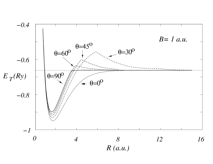
Figure 2: Total energy $E_{T}$ in Rydbergs of the $(ppe)$-system as function of interproton distance $R$ for different inclinations at $B=2.3505\times 10^{9}\,G\,(\,1a.u.)$

Figure 3: Total energy $E_{T}$ in Rydbergs of the $(ppe)$-system as function of interproton distance $R$ for different inclinations at $B=10^{11}\,G$

Figure 4: Total energy $E_{T}$ in Rydbergs of the $(ppe)$-system as function of interproton distance $R$ for different inclinations at $B=10^{12}\,G$. The result by Wille Wille:1988 is shown by bullet (see text)

Figure 5: Total energy $E_{T}$ in Rydbergs of the $(ppe)$-system as a function of interproton distance $R$ for different inclinations at $B=10^{13}\,G$. Plots for $\theta=45^{o},60^{o},90^{o}$ consist of two parts – (i) solid line, when $d$ is kept fixed, $d=0$ (gauge center coincides with the mid-point between protons) and which displays a minimum, and (ii) the dotted line is the result of minimization, when the parameter $d$ is released.

However, the situation is drastically different for $B>10^{11}\,G$, see Figs. 4-5. There exists a certain critical angle $\theta_{cr}$, such that for $\theta<\theta_{cr}$ the situation remains similar to that given above – each potential curve is characterized by a well-pronounced minimum at finite $R$. With increase of the inclination, at $\theta\gtrsim\theta_{cr}$ the minimum in the total energy first becomes very shallow with $E_{T}>E_{H}$ and ceases to exist at all. We were unable to localize with a confidence the domain in $R$ which correspond to a shallow minimum which leads to the possible dissociation $H_{2}^{+}\rightarrow H+p\,$ that was predicted in Larsen as well as being discussed in our previous work Turbiner:2001 . We consider that the prediction of dissociation for large inclinations emerged as an artifact of an improper choice of the gauge fixing (see the discussion above). A detailed study of the transition domain (existence $\leftrightarrow$ non-existence) of $H_{2}^{+}$ is beyond of scope of the present article. In any case, such a study requires much more accurate quantitative techniques as well as a sophisticated qualitative analysis. Schematically, the situation is illustrated in Fig. 6.

Figure 6: $H_{2}^{+}$-ion: domains of existence $\leftrightarrow$ non-existence for the $1_{g}$ state.

Figure 7a: The dependence $d$ vs $R$ at $B=1\,a.u.$ for different inclinations $\theta\neq 0^{o}$.

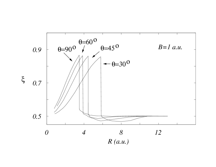
Figure 7b: The dependence $\xi$ vs $R$ at $B=1\,a.u.$ for different inclinations $\theta\neq 0^{o}$.

Figure 8a: The dependence $d$ vs $R$ at $B=10^{12}\,G$ for different inclinations $\theta\neq 0^{o}$.

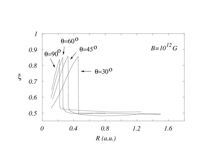
Figure 8b: The dependence $\xi$ vs $R$ at $B=10^{12}\,G$ for different inclinations $\theta\neq 0^{o}$.

It is quite interesting to explore the variation of the vector potential (2) for $\theta\neq 0^{o}$, in particular, the position of the gauge center as a function of interproton distance $R$ and magnetic field . In Figs. 7 a,b for $B=1a.u.$ and Figs. 8 a,b for $10^{12}\,G$, correspondingly, both the $\xi-$ and $d-$ dependence are presented (see (2) and discussion in Sec.III). This dependence is very similar for all magnetic fields studied. It is worthwhile to emphasize that for all the potential curves given the minimum (in other words, the equilibrium position) at $R=R_{eq}$ somehow corresponds to a gauge close to the symmetric gauge: $\xi\gtrsim 1/2$ and $Y=Z=0\,(d=0)$. A similar situation holds for small interproton distances, $R<R_{eq}$. However, for large $R,R>R_{eq}$ the parameter $\xi$ grows smoothly, reaching a maximum near the maximum of the potential curve which we denote by $R=R_{cr}$. It then falls sharply to the value $\xi\sim 1/2$. In turn, the parameter $d$ remains equal 0 up to $R=R_{cr}$ (which means the gauge center coincides to the mid-point between protons), then sharply jumps to 1 (gauge center coincides with the position of a proton), displaying a behavior similar to a phase transition. It is indeed a type of phase transition behavior stemming from symmetry breaking: from the domain $R<R_{cr}$, where the permutation symmetry of the protons holds and where the protons are indistinguishable, to the domain $R>R_{cr}$, where this symmetry does not exist and electron is attached to one particular proton. Such a type of ‘phase transitions’ is typical in chemistry and is called a ‘chemical reaction’. Hence the parameter $R_{cr}$ characterizes a distance at which the chemical reaction $H_{2}^{+}\rightarrow H+p$ starts. Somewhat similar behavior of the gauge parameters has appeared in the study of the exotic $H_{3}^{2+}$-ion Lopez-Tur:2002 .

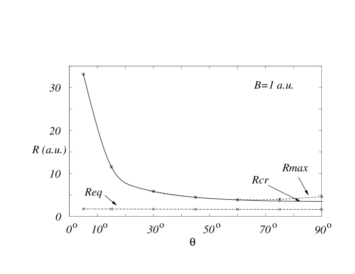
Figure 9: The dependence of $R_{crit}$ and position of the maximum $R_{max}$ compared to the equilibrium position $R_{eq}$ at $B=1a.u.$ for different inclinations $\theta$.

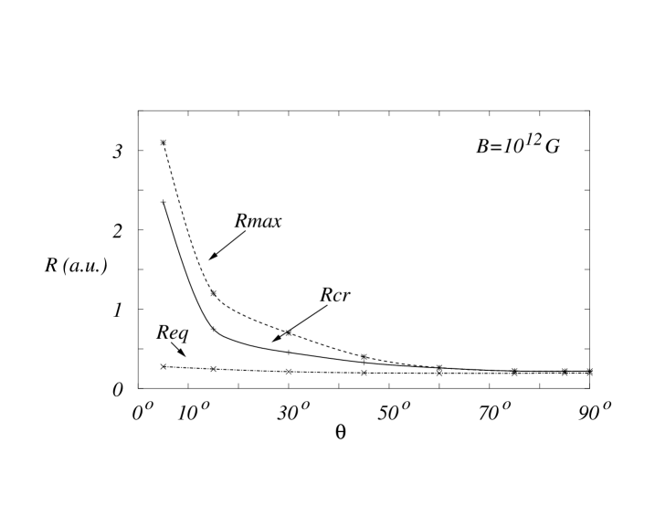
Figure 10: The dependence of $R_{crit}$ and position of the maximum $R_{max}$ compared to the equilibrium position $R_{eq}$ at $B=10^{12}\,G$ for different inclinations $\theta$.

In Figs. 9-10 the behaviors of $R_{eq},R_{max},R_{cr}$ vs inclination at $B=1a.u.$ and $10^{12}\,G$ are displayed. The behavior of $R_{eq}$ vs $\theta$ demonstrates almost no dependence on $\theta$ in contrast to both $R_{max}$ and $R_{cr}$ which drastically decrease with the growth of $\theta$. We do not have a reliable physical explanation of this behavior.

The total energy dependence of $H_{2}^{+}$ (at $R=R_{eq}$) as a function of the inclination angle $\theta$ for different magnetic fields is shown in Fig. 11. The dotted line corresponds to the $H$-atom total energy in the corresponding magnetic field. For weak magnetic fields the hydrogen atom total energy is always higher than that of the $H_{2}^{+}$-ion. However, for $B\gtrsim 2\times 10^{11}\,G$ the situation changes – a minimum of the $H_{2}^{+}$ total energy for angles $\theta>\theta_{cr}$ does not exist any more. Surprisingly, $\theta_{cr}$ corresponds approximately to the moment when the total energy of the $H$-atom becomes equal to the total energy of the $H_{2}^{+}$-ion. If the form of vector potential (2) is kept fixed with $\xi=1/2$ and $Y=Z=0\,(d=0)$, then a spurious minimum appears; its position is displayed by the dotted curve. However, if the gauge center parameters are released this minimum disappears (see the discussion above). It was an underlying reason for the erroneous statement about the existence of the unstable $H_{2}^{+}$ ion in this domain with a possibility to dissociate $H_{2}^{+}\rightarrow H+p$ (see Turbiner:2001 ). For all magnetic fields studied the total energy is minimal at $\theta=0^{o}$ (parallel configuration) and then increases monotonically with inclination in complete agreement with statements of other authors Wille:1988 ; Kher ; Larsen ; Schmelcher .

$$\begin{array}[]{cc}{\includegraphics[width=173.44756pt,angle={-90}]{EvsthetaB9.ps}}&{\includegraphics[width=173.44756pt,angle={-90}]{EvsthetaB12.ps}}\\ {\includegraphics[width=173.44756pt,angle={-90}]{EvsthetaB10.ps}}&{\includegraphics[width=173.44756pt,angle={-90}]{EvsthetaB13.ps}}\\ {\includegraphics[width=173.44756pt,angle={-90}]{EvsthetaB11.ps}}&{\includegraphics[width=173.44756pt,angle={-90}]{EvsthetaBNR.ps}}\end{array}$$

Figure 11: $H_{2}^{+}$ total energy ($E_{T}$) for the ground state $1_{g}$ as function of the inclination angle $\theta$ for different magnetic fields. The dotted lines correspond to the H-atom total energy taken from Salpeter:1992 . Dashed lines describe a total energy corresponding to a spurious minimum (see discussion in the text).

In a similar way the binding energy $E_{b}=B-E_{T}$, as well as the dissociation energy (affinity to a hydrogen atom) $E_{d}=E_{H}-E_{T}$ as a function of $\theta$ always decreases when changing from the parallel to the perpendicular configuration (see Fig. 11). Such behavior holds for all values of the magnetic field strength studied. Thus, we can draw the conclusion that the molecular ion becomes less and less stable monotonically as a function of inclination angle. This confirms the statement made in Kher ; Wille:1988 ; Larsen ; Schmelcher , that the highest molecular stability of the $1_{g}$ state of $H_{2}^{+}$ occurs for the parallel configuration. Thus, the $H_{2}^{+}$ molecular ion is the most stable in parallel configuration.

We extend the validity of this statement to magnetic field strengths $10^{13}<B\lesssim 4.414\times 10^{13}\,G$. It is worth emphasizing that the rate of increase of binding energy $E_{b}$ with magnetic field growth depends on the inclination – it slows down with increased inclination. This effect implies that the $H_{2}^{+}$-ion in the parallel configuration becomes more and more stable against rotations – the energy of the lowest rotational state increases rapidly with magnetic field (see Table V below and the discussion there).

Regarding the interproton equilibrium distance $R_{eq}$, one would naively expect that it would always decrease with inclination (see Fig. 12). Indeed, for all the magnetic fields studied we observe that $R_{eq}$ at $\theta=0^{\circ}$ is larger than for any $\theta\neq 0^{\circ}$ (see below, Tabs. I, II, III). This can be explained as a natural consequence of the much more drastic shrinking of the electronic cloud in the direction transverse to the magnetic field than in the longitudinal one. Actually, for magnetic fields $B\lesssim 10^{12}\,G$ the equilibrium distance $R_{eq}$ decreases monotonically with inclination growth until it reaches $\theta_{cr}$, as seen in Fig. 12. As mentioned above, if the parameters of the vector potential (2) are kept fixed, $\xi=1/2$ and $Y=Z=0\,(d=0)$, a spurious minimum appears and generates anomalous (spurious) $R_{eq}$ behavior for $\theta>\theta_{cr}$(see Turbiner:2001 ).

$$\begin{array}[]{cc}\includegraphics[width=173.44756pt,angle={-90}]{RvsthetaB9.ps}&\includegraphics[width=173.44756pt,angle={-90}]{RvsthetaB12.ps}\\ \includegraphics[width=173.44756pt,angle={-90}]{RvsthetaB10.ps}&\includegraphics[width=173.44756pt,angle={-90}]{RvsthetaB13.ps}\\ \includegraphics[width=173.44756pt,angle={-90}]{RvsthetaB11.ps}&\includegraphics[width=173.44756pt,angle={-90}]{RvsthetaBNR.ps}\end{array}$$

Figure 12: $H_{2}^{+}$ equilibrium distance as function of the inclination angle $\theta$ for the $1_{g}$ state. Dashed lines describe the position of a spurious minimum (see discussion in the text and Fig. 11).

In Tabs. I, II and III the numerical results for the total energy $E_{T}$, binding energy $E_{b}$ and equilibrium distance $R_{eq}$ are displayed for $\theta$=0^∘, $45^{\circ}$ and $90^{\circ}$, respectively. As seen in Table I, our results for $\theta=0^{\circ}$ lead to the largest binding energies for $B>10^{11}\,G$ in comparison with previous calculations. For $B\lesssim 10^{11}\,G$, our binding energies for the parallel configuration appear to be very close (of the order of $\lesssim 10^{-4}-10^{-5}$ in relative deviation) to the variational results by Wille Wille:1988 , which are the most accurate so far in this region of magnetic field strengths. Those results are based on the use of a trial function in the form of a linear superposition of $\sim 500$ Hylleraas type functions. It is quite striking that our simple trial function (8) with ten variational parameters gives comparable (for $B\lesssim 10^{11}\,G$) or even better (for $B>10^{11}\,G$) accuracy. It is important to reveal the reason why the trial function Wille:1988 fails to be increasingly inaccurate with magnetic field growth for $B>10^{11}\,G$. An explanation of this inaccuracy is related to the fact that in the $(x,y)$- directions the exact wave function decays asymptotically as a Gaussian function, unlike the Hylleraas functions which decay as the exponential of a linear function. The potential corresponding to the function Wille:1988 reproduces correctly the original potential near Coulomb singularities but fails to reproduce $\sim\rho^{2}$-growth at large distances. This implies a zero radius of convergence of the perturbation theory for which the variational energy represents the first two terms (see discussion in Tur ).

Table 1: Total, $E_{T}$, binding, $E_{b}$, energies and equilibrium distance $R_{eq}$ for the state $1_{g}$ in the parallel configuration, $\theta=0^{\circ}$. ^† This value is taken from Lopez:1997

$B$	$E_{T}$ (Ry)	$E_{b}$ (Ry)	$R_{eq}$ (a.u.)
$B=0$	-1.20525	—	1.9971	Present†
	-1.20527	—	1.997	Wille Wille:1988
$10^{9}\,G$	-1.15070	1.57623	1.924	Present
	-1.15072	1.57625	1.924	Wille Wille:1988
$1\,a.u.$	-0.94991	1.94991	1.752	Present
	—	1.9498	1.752	Larsen Larsen
	-0.94642	1.94642	1.76	Kappes et al Schmelcher
$10^{10}\,G$	1.09044	3.16488	1.246	Present
	1.09031	3.16502	1.246	Wille Wille:1988
$10\,a.u.$	5.65024	4.34976	0.957	Present
	—	4.35	0.950	Wille Wille:1988
	—	4.35	0.958	Larsen Larsen
	—	4.3346	0.950	Vincke et al Vincke
$10^{11}\,G$	35.0434	7.50975	0.593	Present
	35.0428	7.5104	0.593	Wille Wille:1988
	—	7.34559	0.61	Lai et al Salpeter:1992
$100\,a.u.$	89.7090	10.2904	0.448	Present
	—	10.2892	0.446	Wille Wille:1988
	—	10.1577	0.455	Wunner et al Wunner:82
	—	10.270	0.448	Larsen Larsen
	—	10.2778	0.446	Vincke et al Vincke
$10^{12}\,G$	408.3894	17.1425	0.283	Present
	—	17.0588	0.28	Lai et al Salpeter:1992
	408.566	16.966	0.278	Wille Wille:1988
$1000\,a.u$	977.2219	22.7781	0.220	Present
	—	21.6688	0.219	Wille Wille:1988
	—	22.7069	0.221	Wunner et al Wunner:82
	—	22.67	0.222	Larsen Larsen
	—	22.7694	0.219	Vincke et al Vincke
$10^{13}\,G$	4219.565	35.7539	0.147	Present
	4231.82	23.52	0.125	Wille Wille:1988
	—	35.74	0.15	Lai et al Salpeter:1992
$4.414\times{10}^{13}\,G$	18728.48	54.4992	0.101	Present

The results for $\theta=45^{\circ}$ are shown in Table II, where a gradual shortening of the equilibrium distance is accompanied by an increase of total and binding energies with magnetic field. It is worth noting that the parameter $\xi$ evolves from about $0.5$ to $0.93$ with magnetic field growth, thus changing from the symmetric gauge for weak fields to an almost asymmetric one for strong ones. This phenomenon takes place for all orientations $0<\theta<\theta_{cr}$, becoming more and more pronounced with increasing inclination angle (see below). We are unaware of any other calculations for $\theta=45^{\circ}$ to compare ours with.

Table 2: Total $E_{T}$, binding $E_{b}$ energies and equilibrium distance $R_{eq}$ for the $1_{g}$ state at $\theta=45^{\circ}$. Optimal value of the gauge parameter $\xi$ is given and $d=0$ is assumed (see text).

$B$	$E_{T}$ (Ry)	$E_{b}$ (Ry)	$R_{eq}$ (a.u.)	$\xi$
$10^{9}$ G	-1.14248	1.56801	1.891	0.5806
$1$ a.u.	-0.918494	1.918494	1.667	0.5855
$10^{10}$ G	1.26195	2.99337	1.103	0.5958
$10$ a.u.	6.02330	3.97670	0.812	0.6044
$10^{11}$ G	36.15633	6.39686	0.466	0.6252
$100$ a.u.	91.70480	8.29520	0.337	0.6424
$10^{12}$ G	413.2987	12.2332	0.198	0.6890
$1000$ a.u.	985.1956	14.8044	0.147	0.7151

For the perpendicular configuration $\theta=90^{\circ}$, the results are presented in Table III. Similar to what appeared for the parallel configuration (see above) our results are again slightly less accurate than those of Wille Wille:1988 for $B\lesssim 10^{10}\,G$, but becoming the most accurate results for stronger fields. In particular, it indicates that the domain of applicability of a trial function in the form of a superposition of Hylleraas type functions, becomes smaller as the inclination grows. The results reported by Larsen Larsen and by Kappes-Schmelcher Schmelcher are slightly worse than ours, although the difference is very small. The evolution of the gauge parameters follow a similar trend, as was observed at $\theta=45^{\circ}$. In particular, $\xi$ varies from $\xi=0.64$ to $\xi=0.98$ with magnetic field growth from $B=10^{9}\,G$ to $B\sim 2\times 10^{11}\,G$ . We should emphasize that the results of Larsen Larsen and Wille Wille:1988 for $B>10^{11}\,G$ do not seem relevant because of loss of accuracy, since the $H_{2}^{+}$ ion does not exist in this region.

Table 3: Total, $E_{T}$, and binding, $E_{b}$, energies and the equilibrium distance $R_{eq}$ for the $1_{g}$ state in the perpendicular configuration, $\theta=90^{\circ}$. The optimal value of the gauge parameter $\xi$ is presented and $d$ is kept fixed, $d=0$ (see text).

$B$	$E_{T}$ (Ry)	$E_{b}$ (Ry)	$R_{eq}$ (a.u.)	$\xi$
$10^{9}$ G	-1.137342	1.56287	1.875	0.6380	Present
		1.56384	1.879		Wille Wille:1988
$1$ a.u.	-0.89911	1.89911	1.635	0.6455	Present
	—	1.8988	1.634		Larsen Larsen
	-0.89774	1.8977	1.65		Kappes et al Schmelcher
$10^{10}$ G	1.36207	2.89324	1.059	0.6621	Present
	—	2.8992	1.067		Wille Wille:1988
$10$ a.u.	6.23170	3.76830	0.772	0.6752	Present
	—	3.7620	0.772		Larsen Larsen
$10^{11}$ G	36.7687	5.78445	0.442	0.7063	Present
	—	5.6818	0.428		Wille Wille:1988
$100$ a.u.	92.7346	7.26543	0.320	0.7329	Present
	—	7.229	0.320		Larsen Larsen
$10^{12}$ G	–	–	–	–	Present
	—	4.558	0.148		Wille Wille:1988
$1000$ a.u.	–	–	–	–	Present
	—	11.58	0.1578		Larsen Larsen

Table 4: The $1_{g}$ state: Expectation values of the transverse $<\rho>$ and longitudinal $<|z|>$ sizes of the electron distribution for the $H_{2}^{+}$-ion in a.u. at different orientations and magnetic field strengths. At $\theta=0^{\circ}$ the expectation value $<\rho>$ almost coincides to the cyclotron radius of the electron.

$B$	$<\rho>$			$<|z|>$
	$0^{o}$	$45^{o}$	$90^{o}$	$0^{o}$	$45^{o}$	$90^{o}$
$10^{9}$ G	0.909	1.002	1.084	1.666	1.440	1.180
$1$ a.u.	0.801	0.866	0.929	1.534	1.313	1.090
$10^{10}$ G	0.511	0.538	0.569	1.144	0.972	0.848
$10$ a.u.	0.359	0.375	0.396	0.918	0.787	0.708
$10^{11}$ G	0.185	0.193	0.205	0.624	0.542	0.514
$10$0 a.u.	0.123	0.129	0.139	0.499	0.443	0.431
$10^{12}$ G	0.060	0.065	–	0.351	0.324	–
$10$00 a.u.	0.039	0.043	–	0.289	0.275	–
$10^{13}$ G	0.019	–	–	0.215	–	–
$4.414\times 10^{13}$ G	0.009	–	–	0.164	–	–

In order to characterize the electronic distribution of $H_{2}^{+}$ for different orientations we have calculated the expectation values of the transverse $<\rho>$ and longitudinal $<|z|>$ sizes of the electronic cloud (see Table IV). Their ratio is always limited,

$$\frac{<\rho>}{<|z|>}\ <\ 1\ ,$$

and quickly decreases with magnetic field growth, especially for small inclination angles. This reflects the fact that the electronic cloud has a more and more pronounced needle-like form oriented along the magnetic line, as was predicted in the classical papers [Kadomtsev:1971, -Ruderman:1971, ]. The behavior of $<\rho>$ itself does not display any unusual properties, smoothly decreasing with magnetic field, quickly approaching the cyclotron radius for small inclinations and large magnetic fields. In turn, the $<|z|>$ monotonically decreases with inclination growth.

As already mentioned, the results of our analysis of the parallel configuration of $H_{2}^{+}$ turned out to be optimal for all magnetic fields studied, being characterized by the smallest total energy. Therefore, it makes sense to study the lowest vibrational and also the lowest rotational state (see Table V). In order to do this we separate the nuclear motion along the molecular axis near equilibrium in the parallel configuration (vibrational motion) and deviation in $\theta$ of the molecular axis from $\theta=0^{\circ}$ (rotational motion). The vicinity of the minimum of the potential surface $E(\theta,R)$ at $\theta=0^{\circ},R=R_{eq}$ is approximated by a quadratic potential, and hence we arrive at a two-dimensional harmonic oscillator problem in the $(R,\theta)$-plane. Corresponding curvatures near the minimum define the vibrational and rotational energies (for precise definitions and discussion see, for example, Larsen ). We did not carry out a detailed numerical analysis, making only rough estimates of the order of $20\%$. For example, at B$=10^{12}\,G$ we obtain $E_{vib}=0.276\,Ry$ in comparison with $E_{vib}=0.259\,Ry$ given in Lopez-Tur:2000 , where a detailed variational analysis of the potential electronic curves was performed. Our estimates for the energy, $E_{vib}$, of the lowest vibrational state are in reasonable agreement with previous studies. In particular, we confirm a general trend of the considerable increase of vibrational frequency with the growth of $B$ indicated for the first time by Larsen Larsen . The dependence of the energy on the magnetic field is much more pronounced for the lowest rotational state – it grows much faster than the vibrational one with magnetic field increase. This implies that the $H_{2}^{+}$-ion in the parallel configuration becomes more stable for larger magnetic fields (see the discussion above). From a quantitative point of view the results obtained by different authors are not in good agreement. It is worth mentioning that our results agree for large magnetic fields $\gtrsim 10\,a.u.$ with results by Le Guillou et al. Legui , obtained in the framework of the so called ‘improved static approximation’, but deviate drastically at $B=1\,a.u.\,$, being quite close to the results of Larsen Larsen and Wille Wille:1987 . As for the energy of the lowest rotational state, our results are in good agreement with those obtained by other authors (see Table V).

Table 5: Energies of the lowest vibrational $(E_{vib})$ and rotational $(E_{rot})$ electronic states associated with the $1_{g}$ state at $\theta=0^{\circ}$. The indexes in Le Guillou et al Legui are assigned to the ‘improved adiabatic approximation’ (a), and to the ‘improved static approximation’ (b).

$B$	$E_{T}$ (Ry)	$E_{vib}$ (Ry)	$E_{rot}$ (Ry)
$10^{9}$ G	-1.15070	0.013	0.0053	Present
	—	0.011	0.0038	Wille Wille:1987
$1$ a.u.	-0.94991	0.015	0.0110	Present
	—	—	0.0086	Wille Wille:1987
	—	0.014	0.0091	Larsen Larsen
	—	0.013	—	Le Guillou et al (a) Legui
	—	0.014	0.0238	Le Guillou et al (b) Legui
$10^{10}$ G	1.09044	0.028	0.0408	Present
	—	0.026	0.0308	Wille Wille:1987
$10$ a.u.	5.65024	0.045	0.0790	Present
	—	0.040	0.133	LarsenLarsen
	—	0.039	—	Le Guillou et al (a) Legui
	—	0.040	0.0844	Le Guillou et al (b) Legui
$10^{11}$ G	35.0434	0.087	0.2151	Present
$100$ a.u.	89.7096	0.133	0.4128	Present
	—	0.141	0.365	LarsenLarsen
	—	0.13	—	Wunner et al Wunner:82
	—	0.128	—	Le Guillou et al (a) Legui
	—	0.132	0.410	Le Guillou et al (b) Legui
$10^{12}$ G	408.389	0.276	1.0926	Present
	—	0.198	1.0375	Khersonskij Kher3
$1000$ a.u.	977.222	0.402	1.9273	Present
	—	0.38	1.77	LarsenLarsen
	—	0.39	—	Wunner et al Wunner:82
	—	0.366	—	Le Guillou et al (a) Legui
	—	0.388	1.916	Le Guillou et al (b) Legui
$10^{13}$ G	4219.565	0.717	4.875	Present
	—	0.592	6.890	Khersonskij Kher3
$4.414\times 10^{13}$G	18728.48	1.249	12.065	Present

In Fig. 13 we show the electronic distributions $\int dy|\psi(x,y,z)|^{2}$ for magnetic fields $10^{9},10^{10},10^{11},10^{12}\,G$ and different orientations for $H_{2}^{+}$ in the equilibrium configuration, $R=R_{eq}$. It was already found explicitly Lopez:1997 that at $\theta=0^{o}$ with magnetic field increase there is a change from ‘ionic’ (two-peak electronic distribution) to ‘covalent’ coupling (one-peak distribution). We find that a similar phenomenon holds for all inclinations. If for $B=10^{9}\,G$, all electronic distributions are characterized by two peaks for all inclinations, then for $B=10^{12}\,G$ all distributions have a single sharp peak. The ‘sharpness’ of the peak grows with magnetic field. Fig. 13 also demonstrates how the change of the type of coupling appears for different inclinations – for larger inclinations a transition $(two-peaks)\leftrightarrow(one-peak)$ appears for smaller magnetic fields. It seems natural that for the perpendicular configuration $\theta=90^{\circ}$, where the equilibrium distance is the smallest, this change appears for even smaller magnetic field.

Figure 13: Electronic distributions $\int dy|\psi(x,y,z)|^{2}$ (normalized to one) for the $1_{g}$ state of $H_{2}^{+}$ (equilibrium configuration) for different magnetic fields and inclinations.

In Figs. 14-18 we present the evolution of the electronic distributions as a function of interproton distance $R$, for inclinations $0^{o},45^{o}$ at $B=1a.u.$ and $10^{12}\,G$ together with the $R$-dependence for the inclination $90^{o}$ at $B=1a.u.\,$. The values of magnetic fields are chosen to illustrate in the most explicit way the situation. In all figures a similar picture is seen. Namely, at not very large magnetic fields $B\lesssim 10^{11}\,G$ and for all inclinations the electronic distribution at small $R<R_{cr}$ is permutationally symmetric and evolves with increase of $R$ from a one-peak to a two-peak picture with more and more clearly pronounced, separated peaks. Then for $R=R_{cr}$ this symmetry becomes broken and the electron randomly chooses one of protons and prefers to stay in its vicinity. For $R\gg R_{cr}$ the electronic distribution becomes totally asymmetric, the electron looses its memory of the second proton. This signals that the chemical reaction $H_{2}^{+}\rightarrow H+p$ has already happened. For larger magnetic fields $B\gtrsim 10^{11}\,G$ for $R<R_{cr}$ the electronic distribution is always single-peaked, a transition from a one-peak to a two-peak picture occurs for $R>R_{cr}$, where the electronic distribution is already asymmetric.

Figure 14: Evolution of the electronic distributions $\int dy|\psi(x,y,z)|^{2}$ (normalized to one) and their contours for the $1_{g}$ state of the $(ppe)$ system with interproton distance for $B=1\,a.u.,\,\theta=0^{o}$.

Figure 15: Evolution of the electronic distributions $\int dy|\psi(x,y,z)|^{2}$ (normalized to one) and their contours for the $1_{g}$ state of the $(ppe)$ system with interproton distance for $B=1\,a.u.,\,\theta=45^{o}$.

Figure 16: Evolution of the electronic distributions $\int dy|\psi(x,y,z)|^{2}$ (normalized to one) and their contours for the $1_{g}$ state of the $(ppe)$ system with interproton distance for $B=1\,a.u.,\theta=90^{o}$.

Figure 17: Evolution of the electronic distributions $\int dy|\psi(x,y,z)|^{2}$ (normalized to one) and their contours for the $1_{g}$ state of the $(ppe)$ system with interproton distance for $B=10^{12}\,G,\theta=0^{o}$.

Figure 18: Evolution of the electronic distributions $\int dy|\psi(x,y,z)|^{2}$ (normalized to one) and their contours for the $1_{g}$ state of the $(ppe)$ system with interproton distance for $B=10^{12}\,G,\theta=45^{o}$.

To complete the study of the $1_{g}$ state we show in Fig. 19 the behavior of the variational parameters of the trial function (9) as a function of the magnetic field strength for the optimal (parallel) configuration, $\theta=0^{o}$. In general, the behavior of the parameters is rather smooth and very slowly-changing, even though the magnetic field changes by several orders of magnitude. This is in drastic contrast with the results of Kappes-Schmelcher Kappes:1994 (see Fig. 1 in this paper). In our opinion such behavior of the parameters of our trial function (9) reflects the level of adequacy (or, in other words, indicates the quality) of the trial function. In practice, the parameters can be approximated by the spline method and then can be used to study magnetic field strengths other than those presented here.

$$\begin{array}[]{c}\begin{picture}(215.0,160.0)(-10.0,0.0)\put(5.0,20.0){$10^{9}$} \put(40.0,20.0){$10^{10}$} \put(83.0,20.0){$10^{11}$} \put(125.0,20.0){$10^{12}$} \put(165.0,20.0){$10^{13}$} \put(85.0,8.0){$B(G)$} \put(-10.0,32.0){$-4$} \put(-10.0,62.0){$-3$} \put(-10.0,92.0){$-2$} \put(-10.0,122.0){$-1$} \put(-10.0,152.0){$\,\,\,0$} \put(150.0,120.0){$A_{2}$} \put(110.0,90.0){$A_{1}$} \put(-10.0,165.0){\includegraphics*[width=166.2212pt,angle={-90}]{A1A2.ps}} \end{picture}\\[-20.0pt] \begin{picture}(215.0,263.0)\put(10.0,20.0){$10^{9}$} \put(45.0,20.0){$10^{10}$} \put(88.0,20.0){$10^{11}$} \put(130.0,20.0){$10^{12}$} \put(170.0,20.0){$10^{13}$} \put(90.0,8.0){$B(G)$} \put(5.0,35.0){$0$} \put(5.0,85.0){$4$} \put(5.0,130.0){$8$} \put(4.0,180.0){$12$} \put(4.0,225.0){$16$} \put(-22.0,155.0){$[a.u.]^{-1}$} \put(170.0,180.0){$\alpha_{3}$} \put(160.0,130.0){$\alpha_{2}$} \put(150.0,80.0){$\alpha_{1}$} \put(140.0,42.0){$\alpha_{4}$} \put(-22.0,0.0){\includegraphics*[width=242.10493pt,height=263.78505pt]{alphas.ps}} \end{picture}\\[-20.0pt] \begin{picture}(215.0,180.0)(-10.0,0.0)\put(5.0,20.0){$10^{9}$} \put(40.0,20.0){$10^{10}$} \put(83.0,20.0){$10^{11}$} \put(125.0,20.0){$10^{12}$} \put(165.0,20.0){$10^{13}$} \put(85.0,8.0){$B(G)$} \put(-12.0,42.0){$0.2$} \put(-12.0,65.0){$0.4$} \put(-12.0,87.0){$0.6$} \put(-12.0,110.0){$0.8$} \put(-12.0,132.0){$1.0$} \put(-12.0,152.0){$1.2$} \put(-35.0,97.0){$[a.u.]^{-1}$} \put(80.0,105.0){$\beta_{2}$} \put(70.0,136.0){$\beta_{3}$} \put(65.0,60.0){$\beta_{1}$} \put(-10.0,167.0){\includegraphics*[width=166.2212pt,angle={-90}]{betas.ps}} \end{picture}\end{array}$$

Figure 19: Variational parameters of the trial function (9) as a function of the magnetic field strength $B$ for the $1_{g}$ state in the parallel configuration, $\theta=0^{\circ}$. In this case $\beta_{1}=\frac{\beta_{1x}}{2}=\frac{\beta_{1y}}{2}\,,\,\beta_{2}=\frac{\beta_{2x}}{2}=\frac{\beta_{2y}}{2}\,,\,\beta_{3}=\frac{\beta_{3x}}{2}=\frac{\beta_{3y}}{2}$ (see eqs.(5,6,8), cf. Lopez:1997 ). The parameter $A_{3}$ is fixed, being equal to $1$ and $\xi=1/2,d=0$ (see text). The error bars correspond to relative deviation in the variational energy in the region $\Delta E_{T}\equiv\frac{E_{T}}{E_{var}}\lesssim~{}10^{-5}$.

V Conclusion

We have carried out an accurate, non-relativistic calculation in the Born-Oppenheimer approximation for the lowest state of the $H_{2}^{+}$ molecular ion for different orientations of the magnetic field with respect to the molecular axis. We studied constant uniform magnetic fields ranging from zero up to $B=4.414\times 10^{13}\,G$, where non-relativistic consideration holds.

For all magnetic fields studied there exist a region of inclinations for which a well-pronounced minimum in the total energy surface for the $1_{g}$ state of the system $(ppe)$ is found. This shows the existence of the $H_{2}^{+}$ molecular ion for magnetic fields $B=0-4.414\times 10^{13}\,G$. The smallest total energy is always found to correspond to the parallel configuration, $\theta=0^{\circ}$, where protons are situated along the magnetic line. The total energy increases, while the binding energy decreases monotonically as the inclination angle grows. The rate of total energy increase as well as binding energy decrease is seen to be always maximal for the parallel configuration. The equilibrium distance exhibits quite natural behavior as a function of the orientation angle $\theta$ – for fixed magnetic field the shorter equilibrium distance always corresponds to the larger $\theta$.

Confirming the qualitative observations made by Khersonskij Kher for the $1_{g}$ state in the contrast to statements in Larsen ; Wille:1988 , we demonstrate accurately that the $H_{2}^{+}$-ion does not exist at a certain range of orientations for magnetic fields $B\gtrsim 2\times 10^{11}\,G$. As the magnetic field increases the region of inclinations where $H_{2}^{+}$ does not exist is seen to broaden, reaching rather large domain $25^{\circ}\lesssim\theta\leqslant 90^{\circ}$ for $B=4.414\times 10^{13}\,G$.

We find that the electronic distributions for $H_{2}^{+}$ in the equilibrium position are qualitatively different for weak and large magnetic fields. In the domain $B<10^{10}\,G$ the electronic distribution for any inclination has a two-peak form, peaking near the position of each proton. On the contrary for $B>10^{11}\,G$ the electronic distribution always has a single peak form with the peak near the midpoint between the protons for any inclination. This implies a physically different structure for the ground state - for weak fields the ground state can be modelled as a ‘superposition’ of hydrogen atom and proton, while for strong fields such modelling is not appropriate.

Unlike standard potential curves for molecular systems in the field-free case, we observe for $\theta>0^{o}$ that each curve has a maximum and approaches to the asymptotics at $R\rightarrow\infty$ from above. The electronic distribution evolves with $R$ from a one-peak form at small $R$ to a two-peak one at large $R$. There exists a certain critical $R_{cr}$ at which one of peaks starts to diminish, manifesting a breaking of permutation symmetry between the protons and simultaneously the beginning of the chemical reaction $H_{2}^{+}\rightarrow H+p$.

Combining all the above-mentioned observations we conclude that for magnetic fields of the order of magnitude $B\sim 10^{11}\,G$ some qualitative changes in the behavior of the $H_{2}^{+}$ ion take place. The behavior of the variational parameters also favors this conclusion. This hints at the appearance of a new scale in the problem. It might be interpreted as a signal of a transition to the domain of developed quantum chaos (see, for example, chaos ).