A Model For Infall Around Virialized Halos

Abstract

Motivated by the recent direct detection of cosmological gas infall, we develop an analytical model for calculating the mean density profile around an initial overdensity that later forms a dark matter halo. We account for the problem of peaks within peaks; when considering a halo of a given mass we ensure that this halo is not a part of a larger virialized halo. For halos that represent high-sigma fluctuations we recover the usual result that such halos preferentially lie within highly overdense regions; in the limit of very low-sigma fluctuations, on the other hand, we show that halos tend to lie within voids. Combined with spherical collapse, our results yield the typical density and velocity profiles of the gas and dark matter that surround virialized halos.

1 Introduction

Numerical simulations of hierarchical halo formation indicate a roughly universal spherically-averaged density profile within virialized dark matter halos (Navarro, Frenk, & White, 1997). Such profiles are generated by complicated processes that involve violent relaxation and multiple shell crossing; the great interest in them results from the possibility of a direct comparison to the profiles inferred from galactic rotation curves (e.g., Salucci & Burkert, 2000; de Blok, McGaugh, & Rubin, 2001; van den Bosch & Swaters, 2001) and from lensing in clusters (e.g., Sand, Treu, & Ellis, 2002; , 2002). However, the analogous question of what is the typical density profile outside the virial radius has received relatively little attention, because of the difficulty of directly observing density profiles even out to the halo virial radius; this difficulty results from the rapid decrease in the gas and dark matter densities with distance from the halo center. However, the theoretical description is simpler for infall outside the virialization radius, since in cold dark matter (hereafter CDM) models there is no shell crossing until the final non-linear collapse.

The gas around halos can only be detected using physical effects that are very sensitive to low-density gas. One such phenomenon is resonant Ly$\alpha$ absorption; Gunn & Peterson (1965) first noted that even an H I neutral fraction $\sim 10^{-5}$ suffices to make gas at the cosmic mean density strongly absorb photons at the Ly$\alpha$ resonance. Thus, the pattern of gas infall around halos may affect observable properties of the Ly$\alpha$ absorption in these regions. At moderate redshifts, these regions near halos play a prominent role in measurements of the proximity effect of quasars (e.g., Scott et al., 2000; Bajtlik, Duncan, & Ostriker, 1988). In these measurements, the effect of the high quasar intensity on the statistics of Ly$\alpha$ absorption is analyzed and used to infer the mean ionizing background, since the quasar intensity dominates only as long as it is significantly stronger than the background. A different application may be possible at very high redshifts, corresponding to the time before the universe was fully reionized; the presence of the fully neutral IGM could be detected through absorption of a bright source by the Ly$\alpha$ damping wing of the IGM (Miralda-Escudé, 1998). However, every bright source creates a surrounding H II region which complicated the interpretation (Cen & Haiman, 2000; Madau & Rees, 2000). The properties of the gas in the regions that lie just outside the host halo of the source galaxy or quasar should play a major role in these various applications of the observed absorption.

The various calculations of absorption cited above neglected the enhanced densities and the negative (i.e., infall) velocities expected for the gas surrounding a massive halo at high redshift. This infall, however, may be an essential component of any correct interpretation of observations; Loeb & Eisenstein (1995) applied it to the proximity effect and showed that neglecting infall can lead to an overestimate of the ionizing background flux by up to a factor of three. Applying the same infall profile, Barkana & Loeb (2002) have recently revealed the signature of infalling gas around high redshift quasars. The spectral pattern due to Ly$\alpha$ absorption by the infalling gas can be used to estimate the quasar’s ionizing intensity and the total mass of its host halo. While the spectra of individual objects are marked by the large density fluctuations expected in the intergalactic medium (hereafter IGM), if this pattern is averaged over many objects then the resulting mean profile could be compared directly with an accurate theoretical prediction for the density and velocity profile of the infalling gas.

Loeb & Eisenstein (1995) defined a halo in the same way as halos were defined in the classic model of Press & Schechter (1974). In this approach, halos on a given scale are defined as forming when the initial density averaged on this scale is higher than a threshold that depends on the collapse redshift and is fixed using spherical collapse. The halo mass function derived from this assumption, when multiplied by an ad-hoc correction factor of two, provides a reasonable match to the results of numerical simulations (e.g., Katz, Quinn, & Gelb, 1993).

The same mass function was later derived by Bond et al. (1991) using a self-consistent approach, with no need for external factors. In their derivation, the factor of two has a more satisfactory origin, namely the so-called “cloud-in-cloud” problem: if the average initial density on a certain scale is above the collapse threshold, this region may be contained within a larger region that is itself also denser than the collapse threshold; in this case the original region should be counted as belonging to the halo with mass corresponding to the larger collapsed region. Bond et al. (1991) and Press & Schechter (1974) both give the same halo mass function and thus appear to be at least statistically valid given the agreement with the mass function seen in numerical simulations. However, the Bond et al. (1991) model is more satisfactory since it accounts for the cloud-in-cloud problem and, more importantly, allows for calculations of other halo properties in addition to simple mass functions, all in an approach that is more self-consistent.

The Bond et al. (1991) approach (also known as extended Press-Schechter) has been used to calculate halo merger histories (Lacey & Cole, 1993), halo mass functions in models with warm dark matter (Barkana, Haiman, & Ostriker, 2001), halo mass functions in a model with ellipsoidal collapse (Sheth, Mo, & Tormen, 2001), and the nonlinear biasing of halos (Porciani et al., 1998; Scannapieco & Barkana, 2002). In this paper, we present a new application of this approach in which we obtain the expected profile of infalling matter around virialized halos. The rest of this paper is organized as follows. In § 2.1 we establish our notation and review the Bond et al. (1991) derivation of the Press & Schechter (1974) halo mass function. In § 2.2 we review the infall profile used by Loeb & Eisenstein (1995) and also derive an alternative model based on similar assumptions but carried out in Fourier space. In § 2.3 we derive our model based on the extended Press-Schechter formalism. In § 2.4 we then discuss the modified picture of halo virialization once infall is included. In § 3 we illustrate the predictions of our model for the initial and final density profiles surrounding halos. Finally in § 4 we give our conclusions.

2 A Model for Infall: Derivation

2.1 Review of Halo Collapse

Before addressing the problem of the initial density profile around a virialized halo, we briefly review in this section the approach of Bond et al. (1991) which leads to the halo mass function. We work with the linear overdensity field $\delta({\bf x},z)\equiv\rho({\bf x},z)/\bar{\rho}(z)-1$, where ${\bf x}$ is a comoving position in space, $z$ is the cosmological redshift and $\rho$ is the mass density, with $\bar{\rho}$ being the cosmic mean density. In the linear regime, the density field maintains its shape in comoving coordinates and the overdensity simply grows as $\delta=\delta_{i}D(z)/D(z_{i})$, where $z_{i}$ and $\delta_{i}$ are the initial redshift and overdensity, and $D(z)$ is the linear growth factor (Peebles, 1980). When the overdensity in a given region becomes non-linear, the expansion halts and the region turns around and collapses to form a virialized halo.

The time at which the region virializes can be estimated based on the initial linear overdensity, using as a guide the collapse of a spherical tophat perturbation. At the moment at which a tophat collapses to a point, the overdensity predicted by linear theory is $\delta_{c}=1.686$ (Peebles, 1980) in the Einstein-de Sitter model. This value depends slightly on cosmological parameters, and even in the Einstein-de Sitter case it is modified by infall, as we discuss in §2.4; our analytical expressions in this section are valid for any value of $\delta_{c}$.

A useful alternative way to view the evolution of density is to consider the linear density field extrapolated to the present time, i.e., the initial density field at high redshift extrapolated to the present by multiplication by the relative growth factor. In this case, the critical threshold for collapse at redshift $z$ becomes redshift dependent,

$$\delta_{c}(z)=\delta_{c}/D(z)\ .$$ (1)

We adopt this view, and throughout this paper the power spectrum $P(k)$ refers to the initial power spectrum, linearly extrapolated to the present (i.e., not including non-linear evolution).

At a given $z$, we consider the smoothed density in a region around a fixed point $A$ in space. We begin by averaging over a large mass scale $M$, and then lower $M$ until we find the highest value for which the averaged overdensity is higher than $\delta_{c}(z)$; we assume that the point $A$ belongs to a halo with a mass $M$ corresponding to this filter scale.

In this picture we can derive the mass distribution of halos at a redshift $z$ by considering the statistics of the smoothed linear density field. If the initial density field is a Gaussian random field and the smoothing is done using sharp $k$-space filters, then the value of the smoothed $\delta$ undergoes a random walk as the cutoff value of $k$ is increased. If the random walk first hits the collapse threshold $\delta_{c}(z)$ at $k$, then at a redshift $z$ the point $A$ is assumed to belong to a halo with a mass corresponding to this value of $k$. Instead of using $k$ or the halo mass, we adopt as the independent variable the variance at a particular filter scale $k$,

$$S_{k}\equiv\frac{1}{2\pi^{2}}\int_{0}^{k}dk^{\prime}\,k^{\prime 2}\,P(k^{\prime})\ .$$ (2)

In order to construct the number density of halos in this approach, we need to solve for the evolution of the probability distribution $Q(\delta,S_{k})$, where $Q(\delta,S_{k})\,d\delta$ is the probability for a given random walk to be in the interval $\delta$ to $\delta+d\delta$ at $S_{k}$. Alternatively, $Q(\delta,S_{k})\,d\delta$ can also be viewed as the trajectory density, i.e., the fraction of the trajectories that are in the interval $\delta$ to $\delta+d\delta$ at $S_{k}$, assuming that we consider a large ensemble of random walks all of which begin with $\delta=0$ at $S_{k}=0$.

Bond et al. (1991) showed that $Q$ satisfies a diffusion equation,

$$\frac{\partial Q}{\partial S_{k}}=\frac{1}{2}\frac{\partial^{2}Q}{\partial\delta^{2}},$$ (3)

which is solved by the Gaussian solution which we label $Q_{0}$:

$$Q_{0}(\delta,S_{k})=\frac{1}{\sqrt{2\pi S_{k}}}\exp\left[-\frac{\delta^{2}}{2\,S_{k}}\right]\ .$$ (4)

To determine the probability of halo collapse at a redshift $z$, we consider the same situation but with an absorbing barrier at $\delta=\nu$, where we set $\nu=\delta_{c}(z)$. The fraction of trajectories absorbed by the barrier up to $S_{k}$ corresponds to the total mass fraction contained in halos with masses higher than the value associated with $S_{k}$. In this case, $Q$ again satisfies eq. (3) and the solution with the barrier in place is given by adding an extra image-solution:

$$Q(\nu,\delta,S_{k})=Q_{0}(\delta,S_{k})-Q_{0}(2\nu-\delta,S_{k}).$$ (5)

Using this expression, the fraction of all trajectories that have passed above the barrier $\nu$ by $S_{k}$ is

$$F(\nu,S_{k})=1-\int_{-\infty}^{\nu}d\delta\,Q(\nu,\delta,S_{k})\ ,$$ (6)

and the differential mass function is found [using eq. (3)] to be

$$f(\nu,S_{k})=\frac{\partial}{\partial S_{k}}F(\nu,S_{k})=\frac{\nu}{\sqrt{2\pi}S_{k}^{3/2}}\exp\left[-\frac{\nu^{2}}{2S_{k}}\right]\ .$$ (7)

As $f(\nu,S_{k})\,dS_{k}$ is the probability that point $A$ is in a halo with mass in the range corresponding to $S_{k}$ to $S_{k}+dS_{k}$, the halo abundance is then simply

$$\frac{dn}{dM}=\frac{\bar{\rho}}{M}\left|\frac{dS_{k}}{dM}\right|f(\nu,S_{k})\ ,$$ (8)

where $dn$ is the comoving number density of halos with masses in the range $M$ to $M+dM$. The cumulative mass fraction in halos above mass $M$ is similarly determined to be

$$F(>M|z)={\rm erfc}\left(\frac{\nu}{\sqrt{2S_{k}}}\right)\ .$$ (9)

While these expressions were derived in reference to density perturbations smoothed by a sharp $k$-space filter as given in eq. (2), $S_{k}$ is often replaced in the final results with the variance of the mass $M$ enclosed in a spatial sphere of comoving radius $r$:

$$\sigma^{2}(M)=\sigma^{2}(r)=\frac{1}{2\pi^{2}}\int_{0}^{\infty}k^{2}dkP(k)W^{2}(kr)\ ,$$ (10)

where $W(x)$ is the spherical tophat window function, defined in Fourier space as

$$W(x)\equiv 3\left[\frac{\sin(x)}{x^{3}}-\frac{\cos(x)}{x^{2}}\right]\ ,$$ (11)

and $M=4\pi\bar{\rho}(0)r^{3}/3$ in terms of the mean density of matter at $z=0$. With these replacements we recover the cumulative mass fraction that was originally derived (Press & Schechter, 1974) simply by considering the distribution of overdensities at a single point, smoothing with a tophat window function, and integrating from $\delta_{c}$ to $\infty$. In this derivation the authors were forced to multiply their result by an arbitrary factor of two, to account for the mass in underdense regions. The excursion-set derivation presented here, based on Bond et al. (1991), properly includes all the mass by accounting for small regions that lie within overdensities on larger scales. This approach also makes explicit the approximations involved in working with $\sigma^{2}(r).$ Strictly speaking, dealing with a real-space filter requires a complete recalculation of $f(\nu,\sigma^{2})$ which accounts for the correlations intrinsic to $W(x)$. However, simply replacing $S_{k}$ with $\sigma^{2}(r)$ in eq. (8) has been shown to be in reasonable agreement with numerical simulations (e.g., Katz, Quinn, & Gelb, 1993), and is thus a standard approximation.

2.2 Infall based on the Press-Schechter Model

In the Press-Schechter model, a halo of mass $M$ is assumed to form at redshift $z$ if the corresponding comoving sphere (of radius denoted $r_{M}$) has a linear overdensity of $\delta=\nu\equiv\delta_{c}(z)$. Loeb & Eisenstein (1995) used this fact to derive a mean infall profile as follows. Consider spheres of various comoving radii $r$, all centered on the region in the initial density field that contains the mass that ends up in the final virialized halo. The mean enclosed overdensity $\delta(r)$ in each such sphere (linearly extrapolated to the present) is a Gaussian variable with variance $\sigma^{2}(r)$ as given in eq. (10). The overdensities in two such spheres with radii $r_{1}$ and $r_{2}$ are correlated with a cross-correlation

$$\xi_{r}(r_{1},r_{2})\equiv\frac{1}{2\pi^{2}}\int_{0}^{\infty}k^{2}dkP(k)W(kr_{1})W(kr_{2})\ .$$ (12)

Thus, the expected value of $\delta(r)$ given that $\delta_{M}\equiv\delta(r_{M})=\nu$ is given by their joint Gaussian distribution as

$$\frac{\langle\delta(r)\rangle_{\rm PS-r}}{\nu}=\frac{\xi_{r}(r_{M},r)}{\sigma^{2}(r_{M})}\ ,$$ (13)

where the notation $PS-r$ indicates a derivation based on the Press-Schechter model and carried out in $r$-space.

In addition to obtaining the mean profile, it is useful to calculate the scatter in the initial profiles around halos of a given mass in order to assess the applicability of the mean profile to individual objects. If in the future the model is to be compared to halos in numerical simulations or in real observations, a quantitative formula for the scatter helps us determine the number of objects necessary to average over before the mean profile emerges. In addition, the scatter itself is a prediction of the model that in principle can be compared to simulations or observations. In the present model, the ratio $\delta(r)/\nu$ follows a Gaussian distribution with the mean value given above and a standard deviation given by

$$\Sigma(r)_{\rm PS-r}=\sqrt{\frac{\sigma^{2}(r)}{\nu^{2}}-\frac{\xi_{r}^{2}(r_{M},r)}{\nu^{2}\sigma^{2}(r_{M})}}\ .$$ (14)

Alternatively, we can create an infall model based on similar assumptions, but (as in the previous subsection) calculated in $k$-space. Consider a halo that forms on a scale with a corresponding variance $S_{k,M}$, and consider a larger scale around it with variance $S_{k}<S_{k,M}$. We obtain here a Press-Schechter model in $k$-space by considering random trajectories but without including an absorbing barrier; the self-consistent inclusion of a barrier, which accounts for peaks-within-peaks and is the hallmark of the extended Press-Schechter model, is considered in the next subsection.

In the absence of a barrier, the probability distribution of the overdensity $\delta$ at any $S_{k}$ is Gaussian, and the values of $\delta$ at multiple points are jointly normal. Now, $\delta$ has variance $S_{k}$ and $S_{k,M}$ at the two scales of interest. Furthermore, since the random walk from $S_{k}$ to $S_{k,M}$ is independent of the random walk from 0 to $S_{k}$, the cross-correlation of the values of $\delta$ at $S_{k}$ and at $S_{k,M}$ is given by the overlapping portion of the two random walks: the cross-correlation is therefore simply $S_{k}$. Similarly to the $r$-space case above, the joint Gaussian distribution yields

$$\frac{\langle\delta(r)\rangle_{\rm PS-k}}{\nu}=\frac{S_{k}}{S_{k,M}}\ .$$ (15)

As in the PS-r model, the distribution of $\delta(r)/\nu$ is Gaussian, where now the standard deviation is

$$\Sigma(r)_{\rm PS-k}=\sqrt{\frac{S_{k}}{\nu^{2}}-\frac{S_{k}^{2}}{\nu^{2}S_{k,M}}}\ .$$ (16)

Note that both of the models developed in this section satisfy the continuity condition $\langle\delta(r)\rangle/\nu\rightarrow 1$ when $r\rightarrow r_{M}$ (or equivalently $S_{k}\rightarrow S_{k,M}$). However, we show in the next section that they fail to give a physically acceptable result in a different limit, when $\nu\ll\sqrt{S_{k,M}}$. Moreover, we have ignored in this section the failure of the simple Press-Schechter approach to account for negative fluctuations, and have not included the factor-of-two normalization fudge factor; in the next section, in contrast, we develop a model that is self-consistent.

2.3 Infall based on the Extended Press-Schechter Model

In this section we derive a new model for the initial density profile around a virialized halo. As additional motivation, we first show that the two simple models considered in the previous section yield results that are physically unacceptable, once we consider the obvious possibility that a small halo will lie within a bigger one. Consider, for example, the PS-r model in a CDM cosmology (the cosmological parameters are listed in section 3). In order to explore the limit of $\nu\ll\sigma(r_{M})$ at $z=0$ (when $\nu=1.68$ in this model), we consider a halo of mass $M=10^{6}M_{\odot}$ ($r_{M}=18$ kpc, $\sigma(r_{M})=8.5$), and a surrounding region with $r=2r_{M}$ ($M(r)=8\times 10^{6}M_{\odot}$, $\sigma(r)=7.4$). Consider randomly chosen regions of size $r$ in the universe. Half of them will have a negative overdensity and half will have a positive overdensity (where, as elsewhere in this paper, we consider the linearly-extrapolated overdensity). Those with a positive perturbation will almost certainly be contained within a halo of mass at least $M(r)$, since the typical $\delta$ on this scale is of order $\sigma(r)$, which in turn is much greater than the threshold $\nu$ for forming a halo. Even for those rare perturbations that are smaller than $\nu$, the fact that the perturbation is positive increases the (already very high) chance for the formation of some halo with radius between $r_{M}$ and $r$. Clearly, among regions with positive perturbations on the scale $r$, very few will contain an isolated halo of size $r_{M}$ that is not contained within a larger halo.

On the other hand, fully half of such large regions have a negative perturbation, again with magnitude of order $\sigma(r)$. Such a negative perturbation implies that certainly no halo has formed on the scale $r$; together with the correlation among spheres of different radii, it also implies a very strong reduction in the chance that any halo has formed on a scale between $r_{M}$ and $r$. This double effect implies that isolated halos of size $r_{M}$ will be found almost exclusively within voids on the scale $r$. Indeed, in the limit of $\nu/\sigma(r_{M})\rightarrow 0$, $\delta$ on the scale $r$ should be negative with a magnitude at least comparable to $\sigma(r_{M})$, in order for $\delta$ to remain negative at all scales from $r$ down to $r_{M}$. Thus, in this limit we should find that the ratio $\delta(r)/\nu\rightarrow-\infty$. This contrasts with the Press-Schechter models from the previous section, which predict that the typical such case should have a positive $\delta$ on the scale $r$ (in fact, a $\delta$ only slightly below $\nu$); this behavior arises from the general failure of these models to properly incorporate negative density fluctuations.

To derive our new, self-consistent model, we apply the extended Press-Schechter model in Fourier space and then use an ansatz to convert it to real space. We begin by following the derivation of $\langle\delta(r)\rangle_{\rm PS-k}$ in the previous subsection but now including the absorption barrier at $\delta=\nu$. Thus, we consider once again the two scales with variances $S_{k,M}$ and $S_{k}$, but we now require $S_{k,M}$ to form a halo that is not contained within any larger virialized halo; in particular this implies that there is no halo on the scale corresponding to $S_{k}$ or on any larger scale. Then the probability distribution of the overdensity $\delta$ at $S_{k}$ is given by $Q(\nu,\delta,S_{k})$ as in eq. (5). As before, the random walk from $S_{k}$ onwards is independent of the random walk leading up to $S_{k}$. In order to account for the extended Press-Schechter definition of halo formation, we use arguments similar to those leading to eq. (7) [see Bond et al. (1991) and Lacey & Cole (1993) for other applications of similar arguments]; the probability distribution of the initial density at $S_{k}$, given the formation of a halo at $S_{k,M}$, is found to be

$$P(\delta|\delta_{M}=\nu)_{\rm ePS-k}=Q(\nu,\delta,S_{k})\,\frac{f(\nu-\delta,S_{k,M}-S_{k})}{f(\nu,S_{k,M})}\ .$$ (17)

The mean expected $\delta$ is given by integrating $\delta$ over this distribution, with limits of $-\infty$ to $+\nu$; we thus obtain the result of using the extended Press-Schechter model in $k$-space:

$$\frac{\langle\delta(r)\rangle_{\rm ePS-k}}{\nu} = 1-\left(1-\alpha+\frac{\alpha}{\beta}\right)\,{\rm erf}\left[\sqrt{\frac{\beta(1-\alpha)}{2\alpha}}\right]$$ (18)

$$-\sqrt{\frac{2\alpha(1-\alpha)}{\pi\beta}}\,\exp\left[-\frac{\beta(1-\alpha)}{2\alpha}\right]\ ,$$

where we have defined

$$\alpha=\frac{S_{k}}{S_{k,M}}\ \ ;\ \ \beta=\frac{\nu^{2}}{S_{k,M}}\ .$$ (19)

Unlike the models in the previous subsection, the present model does not yield a Gaussian probability distribution for the density. To find the scatter, we first integrate the probability distribution given by eq. (17) and find the cumulative probability distribution $P_{C}$. Using the variable $\gamma=\delta/\nu$ instead of $\delta$, the probability of obtaining a value of $\delta(r)$ that is between $-\infty$ and $\nu\gamma$ equals

$$P_{C}(\gamma)_{\rm ePS-k} = 1+\frac{1}{2}\left[{\rm erf}(A)+{\rm erf}(B)\right]$$ (20)

$$+\sqrt{\frac{\alpha}{2\pi\beta(1-\alpha)}}\,\left[e^{-A^{2}}-e^{-B^{2}}\right]\ ,$$

where we use the shorthand

$$A=\frac{(\gamma-\alpha)\sqrt{\beta}}{\sqrt{2\alpha(1-\alpha)}}\ \ ;\ \ B=\frac{(\gamma+\alpha-2)\sqrt{\beta}}{\sqrt{2\alpha(1-\alpha)}}\ .$$ (21)

We can now numerically calculate the $1-\sigma$ interval of $\delta(r)$ by bracketing the central $68.3\%$ of the probability. For a given $M$ and $\nu$, we thus define the minus $1-\sigma$ density profile as given by values of $\gamma$ determined at each $r$ by $P_{C}(\gamma)=15.9\%$, while the plus $1-\sigma$ profile is determined by $P_{C}(\gamma)=84.1\%$.

Having developed several possible infall models, we compare their relative merits by considering several limiting cases. First, when $r\rightarrow r_{M}$ (or equivalently $S_{k}\rightarrow S_{k,M}$), all the models satisfy the continuity condition $\langle\delta(r)\rangle/\nu\rightarrow 1$ with zero scatter. In the limit of $\beta\rightarrow 0$, we require $\langle\delta(r)\rangle/\nu\rightarrow-\infty$ as explained earlier in this section. While $\langle\delta(r)\rangle_{\rm ePS-k}$ behaves correctly in this limit (and approaches a constant that does not depend on $\nu$), $\langle\delta(r)\rangle_{\rm PS-r}$ and $\langle\delta(r)\rangle_{\rm PS-k}$ are proportional to $\nu$ and thus fail to correctly describe the $\beta\rightarrow 0$ limit. Thus, only $\langle\delta(r)\rangle_{\rm ePS-k}$ behaves physically in both of the limits $r\rightarrow r_{M}$ and $\beta\rightarrow 0$.

In the limit of a halo that represents an extremely rare peak, i.e., $\beta\rightarrow\infty$, the Press-Schechter model becomes an accurate description that is equivalent to the extended Press-Schechter model; the reason is that if the central halo is extremely rare then it is exceedingly improbable to find a virialized halo on any scale larger than $r_{M}$, and thus it is acceptable to neglect the barrier at $\delta=\nu$ except right near the scale $r_{M}$. In this limit, $\langle\delta(r)\rangle_{\rm ePS-k}$ and $\langle\delta(r)\rangle_{\rm PS-k}$ both approach the value $\nu\alpha$. However, in this limit only, the PS-r model is the best available model since it directly considers spheres in real space, and these correspond most directly to the regions that actually collapse to form halos; this model also applies most directly to the threshold $\nu$ that is derived based on spherical collapse in real space. Indeed, the best possible model would be $\langle\delta(r)\rangle_{\rm ePS-r}$, a quantity based on the extended Press-Schechter model applied directly in real space. However, such a model would be extremely difficult to develop, since excursion sets of $\delta$ as a function of $\sigma^{2}(r)$ would no longer correspond to pure random walks [see Bond et al. (1991) for related discussion]. Thus, following the tradition of the extended Press-Schechter approach (see §1 and 2.1), we use $\langle\delta(r)\rangle_{\rm ePS-k}$ along with an ansatz.

To arrive at the most logical ansatz, we simply replace $\alpha$ and $\beta$ in eq. (19) with their $r$-space equivalents. Based on the above arguments, we adopt $\langle\delta(r)\rangle_{\rm PS-r}$ and $\Sigma(r)_{\rm PS-r}$ as the correct $\beta\rightarrow\infty$ limits of the mean and the standard deviation, respectively. Indeed, $\delta(r)$ in the ePS-k model approaches a Gaussian distribution in the limit of $\beta\rightarrow\infty$, and therefore we can match this limit identically to the PS-r model, and this procedure fixes unambiguously the required $r$-space versions of both $\alpha$ and $\beta$. Thus, our final ansats for the mean initial profile of the density averaged in spheres of radius $r$, linearly extrapolated to $z=0$, around a virialized halo is

$$\frac{\langle\delta(r)\rangle}{\nu}\equiv\frac{\langle\delta(r)\rangle_{\rm ePS-k}}{\nu}\ ,$$ (22)

where we use eq. (18) except that we define

$$\alpha\equiv\frac{\xi_{r}(r_{M},r)}{\sigma^{2}(r_{M})}\ \ ;\ \ \beta\equiv\frac{\nu^{2}\alpha(1-\alpha)}{\sigma^{2}(r)-\alpha\,\xi_{r}(r_{M},r)}\ .$$ (23)

We apply these same definitions to eqs. (20) and (21) in order to estimate the scatter in the infall profiles as given by this final model.

2.4 Halo Virialization in the Presence of Infall

As noted in §2.1, the linearly extrapolated initial overdensity of a spherical tophat corresponding to the moment of collapse is (Peebles, 1980) $\delta_{c}=3(12\pi)^{2/3}/20$ if $\Omega_{m}=1$. In reality, even a slight violation of the exact symmetry of the initial perturbation can prevent the tophat from collapsing to a point. Instead, the halo reaches a state of virial equilibrium by violent relaxation (phase mixing). Using the virial theorem $U=-2K$ to relate the potential energy $U$ to the kinetic energy $K$ in the final state, the final overdensity relative to the cosmic mean density at the collapse redshift is (Peebles, 1980) $\Delta_{c}=18\pi^{2}$ in the Einstein-de Sitter model. Thus, if a tophat containing mass $M$ is predicted by spherical collapse to reach a physical radius $R=0$ at the collapse redshift $z$, this amount of mass is instead assumed to be distributed within a sphere of size equal to the (physical) virial radius $R_{\rm vir}$ determined by $M=\frac{4}{3}\pi\bar{\rho}(z)\Delta_{c}R_{\rm vir}^{3}$.

In the presence of infall, however, the enclosed mass is modified. Indeed, at the moment when the tophat mass $M$ is predicted by spherical collapse to reach a radius $R=0$, the surrounding infall implies that additional mass has already accumulated within the sphere of radius $R_{\rm vir}$. Thus, the overdensity within the standard virial radius $R_{\rm vir}$ is predicted to be higher than the standard value of $18\pi^{2}$. Therefore, once infall is included, even in the Einstein-de Sitter model the precise overdensity to be used to define a “virialized” halo becomes somewhat uncertain. In this paper we choose the overdensity of $18\pi^{2}$ to define the virial radius in all cosmological models, since this overdensity has been frequently used to compare the analytical model predictions (e.g., for the halo mass function) with numerical simulations (e.g., Jenkins et al., 2001). Thus, we carry out spherical collapse calculations with the average infall profile derived in the previous section. Having fixed the virial overdensity we then find the enclosed virial mass $M_{\rm vir}$, which is greater than the original tophat mass $M$ by up to a factor of two (depending on $M$, $z$, and the cosmological parameters). We also find the linearly extrapolated initial overdensity of the virialized mass shell, which we denote $\delta_{v}$.

In the Einstein-de Sitter case we find $\delta_{v}=1.5927$ for the infall-based definition of virialization just noted, compared to the standard value of $\delta_{c}=1.6865$ for an isolated initial tophat perturbation. More generally, $\delta_{c}$ depends on the cosmological parameters. In a flat cosmology with $\Omega_{m}(z)+\Omega_{\Lambda}(z)=1$ at a redshift $z$, we find the following fitting function accurate to $5\times 10^{-5}$ in the range $0.05<\Omega_{m}(z)<1$ (see also, e.g., Eke, Cole & Frenk, 1996):

$$\delta_{c}=1.6865\left[1+\frac{x}{1000}\left(4.86-.51x-.113x^{2}\right)\right]\ ,$$ (24)

where $x=\log\left[\Omega_{m}(z)\right]$. Although $\delta_{v}$ does not strictly depend only on the cosmological parameters, we find numerically that it is essentially independent of halo mass. Indeed, over a wide parameter range of $10^{4}M_{\odot}<M<10^{16}M_{\odot}$ and $0.05<\Omega_{m}(z)<1$, $\delta_{v}$ is given to within a relative accuracy of $3\times 10^{-4}$ by

$$\delta_{v}=1.5927\left[1+\frac{x}{1000}\left(3.9-.36x-.09x^{2}\right)\right]\ .$$ (25)

Thus, for example, $\delta_{v}=1.573$ for $\Omega_{m}(z)=0.05$, compared to $\delta_{c}=1.659$ in this case.

We note that the Press-Schechter halo mass function is known to underestimate the abundance of rare halos relative to the results of numerical simulations (e.g., Jenkins et al., 2001). This can be fixed in the Einstein-de Sitter model if the collapse threshold is multiplied by a factor of 0.87, while we find that infall lowers the threshold, from $\delta_{c}$ to $\delta_{v}$, by a factor of only 0.94. Thus, infall by itself cannot fully explain the discrepancy in the Press-Schechter prediction for the number of high-mass halos.

3 Results

We illustrate results for the standard cosmological parameters $\Omega_{m}=0.3$, $\Omega_{\Lambda}=0.7$, $h=0.7$ and a CDM power spectrum (with initial slope $n=1$) normalized to a variance $\sigma_{8}=0.8$ in spheres of radius 8 $h^{-1}$ Mpc. We consider a wide range of redshifts but focus on the higher values since at $z<2$ the infalling intergalactic gas is very tenuous and may thus be undetectable; however, note that at low redshift a significant fraction of the infalling baryons may already be in the form of virialized dwarf galaxies that are themselves detectable.

Figure 1 shows the predictions of our model [eqs. (22) and (23)] for the mean initial profiles of enclosed density around virialized halos. In most cases, the profiles lie significantly below the asymptotic case of a rare halo ($\beta\rightarrow\infty$) for which the profile is given by $\langle\delta(r)\rangle_{\rm PS-r}$ as in eq. (13). In particular, when $M_{\rm vir}=10^{8}M_{\odot}$, a halo forming at $z\la 2$ is most likely to be found in a void on all scales larger than a few times $r_{M}$. Note that we restrict all calculations to radii where the initial profile of enclosed density is monotonically decreasing, since otherwise shells would cross during the subsequent collapse; this cutoff affects only the $z=0$ cases as well as the $M_{\rm vir}=10^{8}M_{\odot}$ halo forming at $z=2$ or 3.

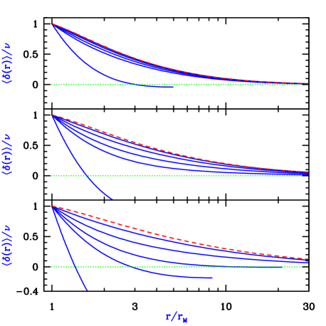
Figure 1: Mean initial density profiles (linearly extrapolated to the present) around virialized halos. Note that $\delta(r)$ is averaged over a sphere of comoving radius $r$, and $r_{M}$ is the initial comoving radius of the tophat. Results are shown for final halo virial masses $M_{\rm vir}=10^{8}M_{\odot}$ (bottom panel), $10^{10}M_{\odot}$ (middle panel), and $10^{12}M_{\odot}$ (top panel). In each case, profiles are shown (solid curves) at $z=0$, 2, 3, 5, and 10, respectively, from bottom to top. Also shown is the asymptotic case of an extremely rare halo (dashed curve). The position of zero overdensity is also indicated (dotted line).

We calculate spherical collapse with the initial profiles shown in Figure 1. The resulting final density profiles are shown in Figure 2. In the limiting case of an extremely rare halo (i.e., very high formation redshift at a fixed halo mass), low mass halos have higher densities of dark matter surrounding their virial radius. This can be understood roughly as follows. For a power spectrum of density fluctuations approximated over some range of scales as a power law $P(k)\propto k^{n}$, the correlation function over the same range of scales varies as $\xi(r)\propto r^{-(n+3)}$. The initial density profile around a rare halo follows, roughly, the dark matter correlation function. On small scales, the CDM power spectrum approaches $n=-3$ and the initial density profile is rather flat, while on larger scales the power index increases toward $n=-2$ for large galaxies, which are therefore surrounded by an initial profile that falls off more steeply (see Figure 1). These differences are magnified by the process of gravitational collapse, resulting in final values for $\rho/\bar{\rho}$ at the virial radius of 41, 34, and 27 for $M_{\rm vir}=10^{8}$, $10^{10}$, and $10^{12}M_{\odot}$, respectively (see Figure 2). However, at moderate redshifts high mass halos represent rarer, more extreme peaks than do low mass halos. Thus, e.g., even at redshift 5 the profile surrounding $M_{\rm vir}\la 10^{10}M_{\odot}$ halos falls significantly below the profile of the extreme limiting case.

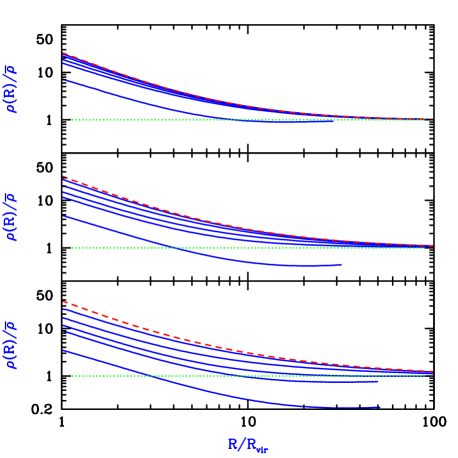
Figure 2: Final density profiles around virialized halos with the initial profiles shown in Figure 1. Note that $\rho(R)$ is the actual density (not enclosed average) at a physical radius $R$, $\bar{\rho}$ is the cosmic mean density at the virialization redshift, and $R_{\rm vir}$ is the final virial radius defined as enclosing a mean density of $18\pi^{2}$ times $\bar{\rho}$. Results are shown for final halo virial masses $M_{\rm vir}=10^{8}M_{\odot}$ (bottom panel), $10^{10}M_{\odot}$ (middle panel), and $10^{12}M_{\odot}$ (top panel). In each case, profiles are shown (solid curves) at $z=0$, 2, 3, 5, and 10, respectively, from bottom to top. Also shown is the asymptotic case of an extremely rare halo (dashed curve). The position of the cosmic mean density is also indicated (dotted line).

Next, we use eq. (20) to predict the expected scatter in the density profiles around virialized halos. Figure 3 shows the initial and final density profiles for $M_{\rm vir}=10^{10}M_{\odot}$ at two different redshifts, for the mean expected profile that we have thus far considered as well as for the plus and for the minus $1-\sigma$ profiles. The final density at $R_{\rm vir}$, for example, is higher than the mean density by a factor of $12^{+8}_{-4}$ at $z=2$ and $28^{+12}_{-7}$ at $z=10$. We thus find a significant scatter, although it is smaller at the higher redshift. If the scatter as calculated within our spherical model is representative of the true scatter among halos, its magnitude suggests that our predicted mean profile can be compared accurately to an observed sample if the sample contains at least a few dozen halos of comparable masses and redshifts.

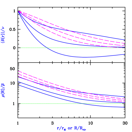
Figure 3: Scatter in the density profiles around virialized halos. Shown are the initial enclosed density profile (top panel) and the final density profile (bottom panel), defined as in Figures 1 and 2, respectively. Each curve fixes the final halo virial mass to $M_{\rm vir}=10^{10}M_{\odot}$, with the halo forming at $z=2$ (solid curves) or $z=10$ (dashed curves). In each case, profiles are shown for the minus $1-\sigma$ profile, the mean expected profile, and the plus $1-\sigma$ profile, respectively, from bottom to top (see text).

Figure 4 shows the final profiles of peculiar velocity $V_{\rm pec}$ of the infalling dark matter corresponding to the halos considered in Figures 1 and 2. The same trends are seen in this figure as in the previous ones; in the extreme case of a rare halo, infall is stronger for low halo masses, but at moderate redshifts, the higher-mass halos actually produce the stronger infall. Figure 4 also shows the peculiar velocity that would correspond to stationary matter, i.e., with zero total velocity (long-dashed curve). This curve is given by minus the Hubble expansion velocity $V_{\rm Hub}$, which in these units is

$$\frac{V_{\rm Hub}(R)}{V_{c}}=\frac{1}{3\pi}\frac{R}{R_{\rm vir}}\ .$$ (26)

Values of $V_{\rm pec}$ that lie below $-V_{\rm Hub}$ give a total velocity corresponding to infall.

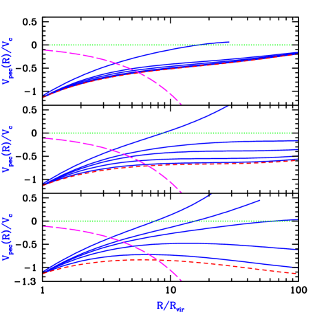
Figure 4: Final velocity profiles around virialized halos with the initial profiles shown in Figure 1. Here $V_{\rm pec}$ is the peculiar velocity (where negative values correspond to infall) at a physical radius $R$, and $V_{c}$ is the circular velocity at the halo virial radius $R_{\rm vir}$. Results are shown for final halo virial masses $M_{\rm vir}=10^{8}M_{\odot}$ (bottom panel), $10^{10}M_{\odot}$ (middle panel), and $10^{12}M_{\odot}$ (top panel). In each case, profiles are shown (solid curves) at $z=0$, 2, 3, 5, and 10, respectively, from top to bottom. Also shown is the asymptotic case of an extremely rare halo (short-dashed curve). For comparison, the curve corresponding to uniform cosmic expansion is shown (dotted line), as well as the curve corresponding to stationary matter (long-dashed curve).

When gas falls into a dark matter halo, incoming streams from all directions strike each other at supersonic speeds, creating a strong shock wave. Three-dimensional hydrodynamic simulations show that the most massive halos at any time in the universe are indeed surrounded by strong, quasi-spherical accretion shocks (Keshet et al., 2002; Abel, Bryan, & Norman, 2002). The radius of this shock depends in general on the history of gas infall into the halo, and will thus vary somewhat among halos depending on the history of their assembly through mergers. In particular, in the spherically-symmetric secondary infall solution, when a trace amount of adiabatic gas is allowed to flow in a gravitational potential determined by collisionless dark matter with density $\Omega_{m}=1$, the accretion shock forms at the radius $R_{90.8}$ which encloses a mean dark matter density of 90.8 times the cosmic mean (Bertschinger, 1985). However, the simulation of Abel, Bryan, & Norman (2002) shows that along most lines of sight the shock occurs at a smaller distance, close to the virial radius.

The position of the accretion shock is an important theoretical prediction that can be probed by observations, since the infalling gas that is about to cross the shock front produces a sharp absorption feature in high-redshift quasar spectra (Barkana & Loeb, 2002). In order to illustrate the range of possible properties of this gas element that lies just beyond the shock front, we use the results mentioned above as a guide and consider two cases for the shock radius $R_{\rm sh}$: the smaller radius $R_{\rm sh}=R_{\rm vir}$ or the larger radius $R_{\rm sh}=R_{90.8}$. We assume that the pressure gradient is negligible in the pre-shock gas compared to gravity, and therefore the gas density and velocity are equal to those of the dark matter at distances beyond the shock front.

Figure 5 shows the density and total infall velocity of the gas that lies just beyond the shock front. The density and the magnitude of the infall velocity both tend to increase with redshift, and follow only weak trends with halo mass at a given redshift. The differences between the two redshifts shown are fairly significant for low mass halos but rather small for high mass halos. In general, the infalling gas is significantly overdense even for halo masses corresponding to $z=0$ dwarf galaxies, especially at the high redshifts which are increasingly becoming the focus of observations. The figure allows us to compare two sources of scatter, namely the varying position of $R_{\rm sh}$ and the variability in the initial density profile. The two effects produce a comparable scatter in the pre-shock density, while the infall velocity, which depends on the enclosed mean density rather than on the density itself, is primarily sensitive to the position of the shock.

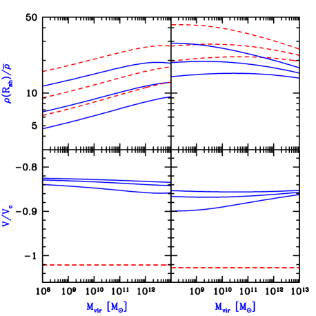
Figure 5: Properties of the infalling gas that is just about to cross the accretion shock around a virialized halo. Shown are the density in units of the cosmic mean (top panels), and the total (not peculiar) velocity in units of the halo circular velocity (bottom panels), both as a function of the final halo virial mass $M_{\rm vir}$. Results are shown at $z=2$ (left panels) and $z=10$ (right panels). Two possible values are considered for the shock radius, $R_{\rm sh}=R_{\rm vir}$ (dashed curves) and $R_{\rm sh}=R_{90.8}$ (solid curves). In each case, profiles are shown for the minus $1-\sigma$ profile, the mean expected profile, and the plus $1-\sigma$ profile, respectively, from bottom to top in the top panels (the order is reversed in the bottom panels).

4 Conclusions

We have developed a model for calculating the initial density profile around overdensities that later collapse to form virialized halos. This is the first such model to account for the possibility that an overdensity on a given scale may be contained inside a large overdensity on an even bigger scale. As a result, we have found that the mean expected profile [eqs. (18) and (23)] depends on both the mass of the halo and its formation redshift. Starting from this mean initial profile, we have used spherical collapse to obtain the final density profile surrounding the virialized halo.

In reality, there will be some variation in the initial profiles, with each leading to a different final profile. We have estimated the scatter within our spherical model, and found that a sample of around a few dozen halos is required in order to obtain an accurate mean profile by averaging. Halo samples derived from numerical simulations or from observations can be used to test our predictions for the mean and for the scatter of the density and velocity profiles of infalling matter around virialized halos.

Once infall is included, the standard derivation of the mean density enclosed within the virial radius fails. Redefining the virial radius as the radius enclosing a density higher than the cosmic mean by the standard value of $18\pi^{2}$, we have found that the initial overdensity needed for a halo to form at some final redshift is lower than it would have to be for an isolated tophat perturbation [compare eqs. (24) and (25)]. Therefore, accounting for infall increases the predicted abundance of rare halos for a given initial power spectrum, but the increase is too small to fully explain the discrepancy between the Press-Schechter prediction for the number of high-mass halos and the number seen in numerical simulations.

We have confirmed that rare halos at a given redshift are surrounded by large, overdense regions of infall, but we have found that the more numerous halos that correspond to low-sigma peaks are surrounded by small infall regions that lie within large voids. However, the infalling gas just beyond the cosmological accretion shock is in general much denser than the cosmic mean; a density larger by a factor of at least 10 occurs around the most massive halos at $z\ga 2$. Possible applications of our results include the Lyman-$\alpha$ absorption profiles of high-redshift objects and the proximity effect of quasars at all redshifts.

References

- Abel, Bryan, & Norman (2002) Abel, T., Bryan, G. L., & Norman, M. L. 2002, Science, 295, 93
- Bajtlik, Duncan, & Ostriker (1988) Bajtlik, S., Duncan, R. C., & Ostriker, J. P. 1988, ApJ, 327, 570
- Barkana, Haiman, & Ostriker (2001) Barkana, R., Haiman, Z., & Ostriker, J. P. 2001, ApJ, 558, 482
- Barkana & Loeb (2002) Barkana, R., & Loeb, A. 2002, Nature, in press
- Bond et al. (1991) Bond, J. R., Cole, S., Efstathiou, G., & Kaiser, N. 1991, ApJ, 379, 440
- Bertschinger (1985) Bertschinger, E. 1985, ApJS, 58, 39
- Cen & Haiman (2000) Cen, R., & Haiman, Z. 2000, ApJL, 542, 75
- (8) Dahle, H., Hannestad, S., & Sommer-Larsen, J. 2002, ApJL, submitted (astro-ph/0206455)
- de Blok, McGaugh, & Rubin (2001) de Blok, W. J. G., McGaugh, S. S., & Rubin, V. C. 2001, AJ, 122, 2396
- Eke, Cole & Frenk (1996) Eke, V. R., Cole, S. & Frenk, C. S. 1996, MNRAS, 282, 263
- Eisenstein & Hu (1999) Eisenstein, D. & Hu, W. 1999, ApJ, 511, 5
- Gunn & Peterson (1965) Gunn, J. E., & Peterson, B. A. 1965, ApJ, 142, 1633
- Jenkins et al. (2001) Jenkins, A. et al. 2001, MNRAS, 321, 372
- Katz, Quinn, & Gelb (1993) Katz, N., Quinn, T., & Gelb, J. M. 1993, MNRAS, 265, 689
- Keshet et al. (2002) Keshet, U., Waxman, E., Loeb, A., Springel, V., & Hernquist, L. 2002, ApJ, in press (preprint astro-ph/0202318)
- Lacey & Cole (1993) Lacey, C., & Cole, S. 1993, MNRAS, 262, 627
- Loeb & Eisenstein (1995) Loeb, A., & Eisenstein, D. J. 1995, ApJL, 448, 17
- Madau & Rees (2000) Madau, P., & Rees, M. J. 2000, ApJL, 542, 69
- Miralda-Escudé (1998) Miralda-Escudé, J. 1998, ApJ, 501, 15
- Navarro, Frenk, & White (1997) Navarro, J. F., Frenk, C. S., & White, S. D. M. 1997, ApJ, 490, 493
- Peebles (1980) Peebles, P. J. E. 1980, The Large-Scale Structure of the Universe (Princeton: Princeton University Press)
- Porciani et al. (1998) Porciani, C., Matarrese, S., Lucchin, F., & Catelan, P. 1998, MNRAS, 298, 1097
- Press & Schechter (1974) Press, W. H., & Schechter, P. 1974, ApJ, 187, 425
- Salucci & Burkert (2000) Salucci, P., & Burkert, A. 2000, ApJ, 537, 9
- Sand, Treu, & Ellis (2002) Sand, D. J., Treu, T., & Ellis, R. S. 2002, ApJ, 574, 129
- Scannapieco & Barkana (2002) Scannapieco, E., & Barkana, R. 2002, ApJ, 571, 585
- Scott et al. (2000) Scott, J., Bechtold, J., Dobrzycki, A., & Kulkarni, V. P. 2000, ApJS, 130, 67
- Sheth, Mo, & Tormen (2001) Sheth, R. K., Mo, H. J., & Tormen, G. 2001, MNRAS, 323, 1
- van den Bosch & Swaters (2001) van den Bosch, F. C., & Swaters, R. A. 2001, MNRAS, 325, 1017