Evolution of Magnetic Fields around a Kerr Black Hole

Abstract

The evolution of magnetic fields frozen to a perfectly conducting plasma fluid around a Kerr black hole is investigated. We focus on the plunging region between the black hole horizon and the marginally stable circular orbit in the equatorial plane, where the centrifugal force is unable to stably balance the gravitational force. Adopting the kinematic approximation where the dynamical effects of magnetic fields on the fluid motion are ignored, we exactly solve Maxwell’s equations with the assumptions that the geodesic motion of the fluid is stationary and axisymmetric, the magnetic field has only radial and azimuthal components and depends only on time and radial coordinates. We show that the stationary state of the magnetic field in the plunging region is uniquely determined by the boundary conditions at the marginally stable circular orbit. If the magnetic field at the marginally stable circular orbit is in a stationary state, the magnetic field in the plunging region will quickly settle into a stationary state if it is not so initially, in a time determined by the dynamical time scale in the plunging region. The radial component of the magnetic field at the marginally stable circular orbit is more important than the toroidal component in determining the structure and evolution of the magnetic field in the plunging region. Even if at the marginally stable circular orbit the toroidal component is zero, in the plunging region a toroidal component is quickly generated from the radial component by the shear motion of the fluid. Finally, we discuss the dynamical effects of magnetic fields on the motion of the fluid in the plunging region. We show that the dynamical effects of magnetic fields are unimportant in the plunging region if they are negligible on the marginally stable circular orbit. This supports the “no-torque inner boundary condition” of thin disks, contrary to the claim in the recent literature.

I Introduction

It is widely believed that accretion disks around Kerr black holes exist in many astrophysical environments, ranging from active galactic nuclei to some stellar binary systems fra02 ; kat98 . People usually assume that the inner boundary of a thin Keplerian disk around a Kerr black hole is located at the marginally stable circular orbit, inside which the centrifugal force is unable to stably balance the gravity of the central black hole nov73 ; pag74 . In the disk region, particles presumably move on nearly circular orbits with a very small inward radial velocity superposed on the circular motion, the gravity of the central black hole is approximately balanced by the centrifugal force. As disk particles reach the marginally stable circular orbit, the gravity of the central black hole becomes to dominate over the centrifugal force and the particles begin to nearly free-fall inwardly. The motion of fluid particles in the plunging region quickly becomes supersonic then the particles loose causal contact with the disk, as a result the torque at the inner boundary of the disk is approximately zero (muc82, ; abr89, ; pac00, ; arm01, ; afs02, , and references therein). This is usually called the “no-torque inner boundary condition” of thin accretion disks.

Some recent studies on the magnetohydrodynamics (MHD) of accretion disks have challenged the “no-torque inner boundary condition”. Magnetic fields have been demonstrated to be the most favorable agent for the viscous torque in an accretion disk transporting angular momentum outward (bal98, , and references therein). By considering the evolution of magnetic fields in the plunging region, Krolik kro99 pointed out that magnetic fields can become dynamically important in the plunging region even though they are not so on the marginally stable circular orbit, and argued that the plunging material might exert a torque to the disk at the marginally stable circular orbit. With a simplified model, Gammie gam99 solved Maxwell’s equations in the plunging region and estimated the torque on the marginally stable circular orbit. He demonstrated that the torque can be quite large and thus the radiation efficiency of the disk can be significantly larger than that for a standard accretion disk where the torque at the inner boundary is zero. Furthermore, Agol and Krolik ago00 have investigated how a non-zero torque at the inner boundary affects the radiation efficiency of a disk.

Numerical simulations of MHD disks haw00 ; arm01 ; haw01a ; haw01b ; haw02 have greatly improved our understanding of disk accretion processes. These simulations show that the magneto-rotational instability effectively operates inside the disk and leads to accretion, though the accretion picture is much more complicated than that assumed in the standard theory of accretion disks. Generally, the disk accretion is non-axisymmetric and strongly time-dependent. It is also found that, as disk material gets into the plunging region, the magnetic stress at the marginally stable circular orbit does not vanish but smoothly extends into the plunging region haw01a ; haw01b ; haw02 , though the effect is significantly reduced as the thickness of the disk goes down arm01 ; haw01a . Furthermore, the specific angular momentum of particles in the plunging region does not remain constant, which implies that the magnetic field may be dynamically important in the plunging region haw01a ; haw01b ; haw02 . All these results are fascinating and encouraging. Unfortunately, due to the limitation in space resolution and time integration, stationary and geometrically thin accretion disks are not accessible to the current 2-D and 3-D simulations. So it remains unclear how much insights we can get for stationary and geometrically thin accretion disks from these simulations afs02 .

Instead of small-scale and tangled magnetic fields in an accretion disk transporting angular momentum within the disk, a large-scale and ordered magnetic field connecting a black hole to its disk may also exist and play important roles in transportation of angular momentum and energy between the black hole and the disk bla98 ; li00a ; li00b ; li02a ; li02b . Recent XMM-Newton observations of some Seyfert galaxies and Galactic black hole candidates provide possible evidences for such a magnetic connection between a black hole and its disk wil01 ; li01 ; mil02 .

All these promote the importance of studying the evolution and the dynamical effects of magnetic fields around a Kerr black hole.

In this paper, we use a simple model to study the evolution of magnetic fields in the plunging region around a Kerr black hole. We assume that around the black hole the spacetime metric is given by the Kerr metric; in the plunging region, which starts at the marginally stable circular orbit and ends at the horizon of the black hole, a stationary and axisymmetric plasma fluid flows inward along timelike geodesics in a small neighborhood of the equatorial plane. The plasma is perfectly conducting and a weak magnetic field is frozen to the plasma. The magnetic field and the velocity field have two components: radial and azimuthal. We will solve the two-dimensional Maxwell’s equations where the magnetic field depends on two variables: time and radius, and investigate the evolution of the magnetic field. This model is similar to that studied by Gammie gam99 , but here we include the time variable. Furthermore, we ignore the back-reaction of the magnetic field on the motion of the plasma fluid to make the model self-consistent, since if the dynamical effects of the magnetic field are important the strong electromagnetic force will make the fluid expand in the vertical direction. The ignorance of the back-reaction of the magnetic field will allow us to to analytically study the evolution of the magnetic field, but it will prevent us from quantitatively studying the dynamical effects of the magnetic field. However, we believe that the essential features of the evolution of the magnetic field in the plunging region is not sensitive to the details of the dynamical effects. To check the self-consistency of the model, we will estimate the dynamical effects of the magnetic field by considering the back-reaction of the magnetic field on the fluid motion. We will also discuss the self-consistent solutions to the coupled Maxwell and dynamical equations, and look for implications to the “no-torque inner boundary condition”.

The paper is organized as follows: In Sec. II we write down the Maxwell’s equations for an ideal MHD plasma. In Sec. III we write down the general forms of the magnetic field and the velocity field of the plasma fluid around a Kerr black hole. In Sec. IV we solve Maxwell’s equations with the approximations outlined above. In Sec. V, with the solutions obtained in Sec. IV, we study the evolution of the magnetic field in the plunging region. In Sec. VI, we check if magnetic fields can become dynamically important in the plunging region. In Sec. VII we draw our conclusions. In the Appendix we solve Maxwell’s equations in the disk region, since we want our solutions in the plunging region to be continuously joined to the solutions in the disk region.

Throughout the paper we use the geometrized units $G=c=1$ and the Boyer-Lindquist coordinates $(t,r,\theta,\phi)$ mis73 ; wal84 , except in the Appendix where cylindrical coordinates are used.

II Maxwell’s equations for an ideal MHD fluid in a curved spacetime

In a curved spacetime, Maxwell’s equations are

$$\nabla_{a}F^{ab}=-4\pi J^{b}\;,$$ (1a)

$$\nabla_{[a}F_{bc]}=0\;,\hskip 14.22636pt$$ (1b)

where $F_{ab}=-F_{ba}$ is the electromagnetic field tensor, $J^{a}$ is the current density 4-vector of electric charge. In Eqs. (1a) and (1b), $\nabla_{a}$ denotes the covariant derivative operator that is compatible with metric: $\nabla_{a}g_{bc}=0$; the square brackets “[ ]” denote antisymmetrization of a tensor.

For an ideal MHD plasma fluid whose electric resistivity is zero, the electric field in the comoving frame is zero, i.e.

$$E_{a}=F_{ab}u^{b}=0\;,$$ (2)

where $u^{a}$ is the 4-velocity of the fluid. In other words, the magnetic field is frozen to the plasma fluid. Then, the electromagnetic field tensor $F_{ab}$ can be written as

$$F_{ab}=-\epsilon_{abcd}B^{c}u^{d}\;,$$ (3)

where $B^{a}$ is the magnetic field measured by an observer comoving with the fluid (i.e., having a 4-velocity $u^{a}$), and $\epsilon_{abcd}$ is the totally antisymmetric tensor of the volume element that is associated with the metric $g_{ab}$. By definition, the magnetic field $B^{a}$ satisfies

$$B^{a}u_{a}=0\;.$$ (4)

The corresponding electromagnetic stress-energy tensor is

$$T_{\rm EM}^{ab}=\frac{1}{4\pi}\left(F^{a}_{\;c}F^{bc}-\frac{1}{4}g^{ab}F_{cd}F^{cd}\right)=\frac{1}{4\pi}B^{2}u^{a}u^{b}+\frac{1}{8\pi}B^{2}g^{ab}-\frac{1}{4\pi}B^{a}B^{b}\;,$$ (5)

where $B^{2}\equiv B_{a}B^{a}$ .

In the case of MHD, the electric current density $J^{a}$ is unknown, but it is only defined by Eq. (1a). The fundamental variables are the electric field $E^{a}$ and the magnetic field $B^{a}$. Maxwell’s equations are then reduced to Eq. (1b). Since in the comoving frame of an ideal MHD flow $E^{a}=0$ and $B^{a}$ is related to the electromagnetic tensor $F_{ab}$ by Eq. (3), the dual of Eq. (1b) gives lic67

$$\nabla_{a}(u^{[a}B^{b]})=0\;.$$ (6)

For an ideal MHD fluid Eqs. (1b) and (6) are equivalent.

Eq. (6) can be expanded as

$$u^{a}\nabla_{a}B^{b}=B^{a}\nabla_{a}u^{b}-B^{b}\nabla_{a}u^{a}+u^{b}\nabla_{a}B^{a}\;.$$ (7)

The contraction of Eq. (7) with $u_{b}$ leads to

$$\nabla_{a}B^{a}-B_{a}a^{a}=0\;,$$ (8)

where $a^{a}\equiv u^{b}\nabla_{b}u^{a}$ is the acceleration of the fluid. In deriving Eq. (8) we have used Eq. (4) and the identity $u_{a}u^{a}=-1$.

Substituting Eq. (8) into Eq. (7), we get

$$u^{a}\nabla_{a}B^{b}=B^{a}\nabla_{a}u^{b}-B^{b}\nabla_{a}u^{a}+u^{b}B_{a}a^{a}\;.$$ (9)

The tensor $\nabla_{a}u_{b}$ is decomposed as haw73

$$\nabla_{a}u_{b}=\frac{1}{3}\Theta h_{ab}+\sigma_{ab}-\omega_{ab}-u_{a}a_{b}\;,$$ (10)

where $h_{ab}\equiv g_{ab}+u_{a}u_{b}$ is the space-projection tensor, $\Theta\equiv h_{ab}\nabla^{a}u^{b}=\nabla_{a}u^{a}$ is the expansion, $\sigma_{ab}\equiv\nabla_{(a}u_{b)}-\Theta h_{ab}/3$ is the shear tensor, and $\omega_{ab}\equiv-\nabla_{[a}u_{b]}$ is the vorticity tensor of the fluid. Here the braces “( )” denote symmetrization of a tensor. It is easy to check that

$$\sigma_{ab}u^{b}=\omega_{ab}u^{b}=0\;,\hskip 28.45274pt\sigma_{ab}h^{ab}=\sigma_{ab}g^{ab}=0\;.$$ (11)

Substituting Eq. (10) into Eq. (9), we obtain

$$u^{a}\nabla_{a}B_{b}=B^{a}(\sigma_{ab}-\omega_{ab})-\frac{2}{3}\Theta B_{b}+B_{a}a^{a}u_{b}\;,$$ (12)

which shows that the evolution of the magnetic field is governed by the expansion, the shear, the vorticity, and the acceleration of the fluid. The contraction of Eq. (12) with $B^{b}$ gives

$$\frac{1}{2}u^{a}\nabla_{a}B^{2}=B^{a}B^{b}\sigma_{ab}-\frac{2}{3}\Theta B^{2}\;,$$ (13)

where we have used $B^{a}B^{b}\omega_{ab}=0$ and Eq. (4).

We note that with the space-projection tensor $h_{ab}$, Eq. (8) can be written as

$$h_{ab}\nabla^{a}B^{b}=0\;,$$ (14)

which says that the spatial divergence of the magnetic field is zero.

In terms of differential forms, the tensor $F_{ab}$ is a closed 2-form, then the Maxwell equation (1b) can be written as $d{\mbox{\boldmath$F$}}=0$ wal84 ; sac77 . Using Stokes’ theorem and Eq. (2), it can be shown that for a perfect conducting fluid the magnetic flux threading any 2-dimensional spatial surface $S$ is unchanged as the surface moves with the fluid

$$\Phi_{B}\equiv\int_{S}{\mbox{\boldmath$F$}}=\mbox{constant}\;.$$ (15)

This is the mathematical formulation for the statement that magnetic field lines are frozen to a perfectly conducting fluid.

III Particle kinematics and magnetic fields around a Kerr black hole

Now let us assume that the background spacetime is the outside of a Kerr black hole of mass $M$ and angular momentum $Ma$, where $-M\leq a\leq M$. In Boyer-Lindquist coordinates, the Kerr metric is mis73 ; wal84

$$ds^{2}=-\left(1-\frac{2Mr}{\Sigma}\right)dt^{2}-\frac{4Mar}{\Sigma}\,\sin^{2}\theta\,dtd\phi+\frac{\Sigma}{\Delta}\,dr^{2}+\Sigma\,d\theta^{2}+\frac{A\sin^{2}\theta}{\Sigma}\,d\phi^{2}\;,$$ (16)

where

$$\Delta\equiv r^{2}-2Mr+a^{2}\;,\hskip 28.45274pt\Sigma\equiv r^{2}+a^{2}\cos^{2}\theta\;,\hskip 28.45274ptA\equiv(r^{2}+a^{2})^{2}-\Delta a^{2}\sin^{2}\theta\;.$$ (17)

A Kerr black hole usually has two event horizons: an inner event horizon and an outer event horizon, whose radii are given by the two roots of $\Delta=0$ . What is relevant in this paper is the outer event horizon, so whenever we talk about the “event horizon” we always mean the outer event horizon, whose radius is

$$r_{\rm H}=M+\left(M^{2}-a^{2}\right)^{1/2}\;.$$ (18)

Let us define an orthonormal tetrad attached to an observer comoving with the frame dragging of the Kerr black hole, $\{e_{0}^{a},e_{1}^{a},e_{2}^{a},e_{3}^{a}\}$, by

$$e_{0}^{a}\equiv\frac{1}{\chi}\left[\left(\frac{\partial}{\partial t}\right)^{a}+\omega\left(\frac{\partial}{\partial\phi}\right)^{a}\right]\;,\hskip 122.34692pt$$

$$e_{1}^{a}\equiv\left(\frac{\Delta}{\Sigma}\right)^{1/2}\left(\frac{\partial}{\partial r}\right)^{a}\;,\hskip 17.07182pte_{2}^{a}\equiv\frac{1}{\Sigma^{1/2}}\left(\frac{\partial}{\partial\theta}\right)^{a}\;,\hskip 17.07182pte_{3}^{a}\equiv\left(\frac{\Sigma}{A}\right)^{1/2}\frac{1}{\sin\theta}\left(\frac{\partial}{\partial\phi}\right)^{a}\;,$$ (19)

where

$$\chi\equiv\left(\frac{\Sigma\Delta}{A}\right)^{1/2}\;,\hskip 28.45274pt\omega\equiv\frac{2Mar}{A}\;,$$ (20)

which are respectively the lapse function and the frame dragging angular velocity. As $r\rightarrow r_{\rm H}$, we have $\chi\rightarrow 0$ and $\omega\rightarrow\Omega_{\rm H}$, where

$$\Omega_{\rm H}=\frac{a}{2Mr_{\rm H}}$$ (21)

is the angular velocity of the event horizon. Then, the 4-velocity of the fluid, $u^{a}$, can be decomposed as

$$u^{a}=\Gamma\left(e_{0}^{a}+v_{\hat{r}}e_{1}^{a}+v_{\hat{\theta}}e_{2}^{a}+v_{\hat{\phi}}e_{3}^{a}\right)\;,$$ (22)

where $(v_{\hat{r}},v_{\hat{\theta}},v_{\hat{\phi}})$ are the components of the 3-velocity of the fluid relative to the observer comoving with the frame dragging, and $\Gamma\equiv(1-v_{\hat{r}}^{2}-v_{\hat{\theta}}^{2}-v_{\hat{\phi}}^{2})^{-1/2}$ is the Lorentz factor. Inserting Eq. (19) into Eq. (22), we have

$$u^{a}=\Gamma\left[\frac{1}{\chi}\left(\frac{\partial}{\partial t}\right)^{a}+v_{\hat{r}}\left(\frac{\Delta}{\Sigma}\right)^{1/2}\left(\frac{\partial}{\partial r}\right)^{a}+\frac{v_{\hat{\theta}}}{\Sigma^{1/2}}\left(\frac{\partial}{\partial\theta}\right)^{a}+\frac{\Omega}{\chi}\left(\frac{\partial}{\partial\phi}\right)^{a}\right]\;,$$ (23)

where

$$\Omega\equiv\omega+\chi v_{\hat{\phi}}\left(\frac{\Sigma}{A}\right)^{1/2}\frac{1}{\sin\theta}$$ (24)

is the angular velocity of the fluid.

The specific angular momentum of a fluid particle is

$$L=\left(\frac{\partial}{\partial\phi}\right)^{a}u_{a}=\frac{\Gamma A\sin^{2}\theta}{\chi\Sigma}(\Omega-\omega)=\Gamma v_{\hat{\phi}}\left(\frac{A}{\Sigma}\right)^{1/2}\sin\theta\;.$$ (25)

Obviously, $L=0$ when $\Omega=\omega$. Thus, an observer comoving with the frame dragging of a Kerr black hole has zero angular momentum bar72 . The specific energy of a fluid particle is

$$E=-\left(\frac{\partial}{\partial t}\right)^{a}u_{a}=\Gamma\chi+L\omega\;.$$ (26)

In Eq. (26), the term $L\omega$ represents the coupling between the orbital angular momentum of the particle and the frame dragging of the Kerr black hole. When the particle moves on a geodesic, $L$ and $E$ defined above are conserved haw73 ; mis73 ; wal84 .

The magnetic field $B^{a}$, which satisfies Eq. (4), can be decomposed as

$$B^{a}=(B_{\hat{r}}v_{\hat{r}}+B_{\hat{\theta}}v_{\hat{\theta}}+B_{\hat{\phi}}v_{\hat{\phi}})e_{0}^{a}+B_{\hat{r}}e_{1}^{a}+B_{\hat{\theta}}e_{2}^{a}+B_{\hat{\phi}}e_{3}^{a}\;,$$ (27)

from which we have

$$B^{2}\equiv B_{a}B^{a}=B_{\hat{r}}^{2}+B_{\hat{\theta}}^{2}+B_{\hat{\phi}}^{2}-(B_{\hat{r}}v_{\hat{r}}+B_{\hat{\theta}}v_{\hat{\theta}}+B_{\hat{\phi}}v_{\hat{\phi}})^{2}\;.$$ (28)

Inserting Eq. (19) into Eq. (27), we have

$$B^{a} = \frac{1}{\chi}(B_{\hat{r}}v_{\hat{r}}+B_{\hat{\theta}}v_{\hat{\theta}}+B_{\hat{\phi}}v_{\hat{\phi}})\left[\left(\frac{\partial}{\partial t}\right)^{a}+\omega\left(\frac{\partial}{\partial\phi}\right)^{a}\right]+B_{\hat{r}}\left(\frac{\Delta}{\Sigma}\right)^{1/2}\left(\frac{\partial}{\partial r}\right)^{a}$$ (29)

$$+\frac{B_{\hat{\theta}}}{\Sigma^{1/2}}\left(\frac{\partial}{\partial\theta}\right)^{a}+\frac{B_{\hat{\phi}}}{\sin\theta}\left(\frac{\Sigma}{A}\right)^{1/2}\left(\frac{\partial}{\partial\phi}\right)^{a}\;;$$

and, correspondingly

$$B_{a} = -\chi(B_{\hat{r}}v_{\hat{r}}+B_{\hat{\theta}}v_{\hat{\theta}}+B_{\hat{\phi}}v_{\hat{\phi}})\,dt_{a}+B_{\hat{r}}\left(\frac{\Sigma}{\Delta}\right)^{1/2}\,dr_{a}$$ (30)

$$+B_{\hat{\theta}}\Sigma^{1/2}\,d\theta_{a}+B_{\hat{\phi}}\left(\frac{A}{\Sigma}\right)^{1/2}\sin\theta\,(d\phi_{a}-\omega dt_{a})\;.$$

IV Solutions of Maxwell’s equations

The Maxwell equations that we want to solve are given by Eq. (6). In terms of coordinate components, Eq. (6) takes a very simple form

$$\frac{1}{\sqrt{-g}}\frac{\partial}{\partial x^{\alpha}}\left[\sqrt{-g}\left(u^{\alpha}B^{\beta}-u^{\beta}B^{\alpha}\right)\right]=0\;,$$ (31)

where $x^{\alpha}=(t,r,\theta,\phi)$, $g$ is the determinant of the metric tensor $g_{\alpha\beta}$, $u^{\alpha}\equiv u^{a}dx_{a}^{\alpha}$ and $B^{\alpha}\equiv B^{a}dx_{a}^{\alpha}$ are respectively

$$u^{t}=\frac{\Gamma}{\chi}\;,\hskip 28.45274ptu^{r}=\Gamma v_{\hat{r}}\left(\frac{\Delta}{\Sigma}\right)^{1/2}\;,\hskip 28.45274ptu^{\theta}=\frac{\Gamma v_{\hat{\theta}}}{\Sigma^{1/2}}\;,\hskip 28.45274ptu^{\phi}=\frac{\Gamma}{\chi}\Omega\;,$$ (32)

and

$$B^{t}=\frac{1}{\chi}(B_{\hat{r}}v_{\hat{r}}+B_{\hat{\theta}}v_{\hat{\theta}}+B_{\hat{\phi}}v_{\hat{\phi}})\;,\hskip 102.43008pt$$

$$B^{r}=B_{\hat{r}}\left(\frac{\Delta}{\Sigma}\right)^{1/2}\;,\hskip 28.45274ptB^{\theta}=\frac{B_{\hat{\theta}}}{\Sigma^{1/2}}\;,\hskip 28.45274ptB^{\phi}=\frac{B_{\hat{\phi}}}{\sin\theta}\left(\frac{\Sigma}{A}\right)^{1/2}+\omega B^{t}\;.$$ (33)

Because of the constraint Eq. (4), among the four equations of (31) only three are independent.

Since the background spacetime is stationary and axisymmetric, we can look for stationary and axisymmetric solutions with $\partial/\partial t=\partial/\partial\phi=0$. However, since we are interested in the time evolution of magnetic fields, we will keep the $\partial/\partial t$ terms on magnetic fields but adopt that $\partial/\partial\phi=0$. To simplify the problem, we further assume that in a small neighborhood of the equatorial plane (i.e., $|\pi/2-\theta|\ll 1$), $u^{\theta}=B^{\theta}=0$ (i.e., $v_{\hat{\theta}}=B_{\hat{\theta}}=0$). This assumption, which has also been used by Gammie gam99 , ensures that $\partial u^{\theta}/\partial\theta=\partial B^{\theta}/\partial\theta=0$ on the equatorial plane. We emphasize that, when $\partial/\partial t\neq 0$, this assumption holds only if the fluid moves geodesically, which requires that the magnetic fields are weak and their dynamical effects are negligible. Otherwise the electromagnetic force will make $u^{\theta}$ and $B^{\theta}$ non-zero except exactly on the equatorial plane. Thus, hereafter we assume that fluid particles move on timelike geodesics in the plunging region. This assumption will be justified latter.

Now, let us focus on solutions on the equatorial plane ($\theta=\pi/2$). Considering the fact that for the Kerr metric $\sqrt{-g}=\Sigma\sin\theta=r^{2}$ on the equatorial plane, Eq. (31) is reduced to

$$\frac{\partial}{\partial t}\left[r^{2}(u^{t}B^{\beta}-u^{\beta}B^{t})\right]+\frac{\partial}{\partial r}\left[r^{2}(u^{r}B^{\beta}-u^{\beta}B^{r})\right]=0\;.$$ (34)

For $\beta=r,t$, Eq. (34) gives

$$\frac{\partial}{\partial t}\left[r^{2}(u^{r}B^{t}-u^{t}B^{r})\right]=0\;,\hskip 28.45274pt\frac{\partial}{\partial r}\left[r^{2}(u^{r}B^{t}-u^{t}B^{r})\right]=0\;,$$ (35)

respectively. The solution of Eq. (35) is

$$u^{t}B^{r}-u^{r}B^{t}=\frac{C_{0}}{r^{2}}\;,$$ (36)

where $C_{0}$ is a constant. With Eq. (15), it can be checked that $2\pi C_{0}\Delta\theta$ is the magnetic flux threading the 2-dimensional surface defined by $t={\rm constant}$, $r={\rm constant}$, $\left|\frac{\pi}{2}-\theta\right|\leq\frac{\Delta\theta}{2}$ and $0\leq\phi<2\pi$.

For $\beta=\theta$, Eq. (34) is automatically satisfied since $u^{\theta}=B^{\theta}=0$ in a small neighborhood of the equatorial plane everywhere and all the time.

For $\beta=\phi$, Eq. (34) gives

$$\frac{\partial}{\partial t}\left[r^{2}(u^{t}B^{\phi}-u^{\phi}B^{t})\right]+\frac{\partial}{\partial r}\left[r^{2}(u^{r}B^{\phi}-u^{\phi}B^{r})\right]=0\;.$$ (37)

From the constraint Eq. (4), we have

$$B^{\phi}=-\frac{1}{u_{\phi}}\left(B^{r}u_{r}+B^{t}u_{t}\right)\;.$$ (38)

Substituting Eq. (36) for $B^{t}$ into Eq. (38), we obtain

$$B^{\phi}=-\frac{1}{u^{r}u_{\phi}}\left[(u^{t}u_{t}+u^{r}u_{r})B^{r}-\frac{C_{0}u_{t}}{r^{2}}\right]\;.$$ (39)

Now, substitute Eq. (36) for $B^{t}$ and Eq. (39) for $B^{\phi}$ into Eq. (37), we obtain a first order partial differential equation

$$\left(u^{t}\frac{\partial}{\partial t}+u^{r}\frac{\partial}{\partial r}\right)\Psi(t,r)=0\;,$$ (40)

where

$$\Psi(t,r)\equiv\frac{1}{u_{\phi}}(r^{2}B^{r}+C_{0}u_{t})\;.$$ (41)

In deriving Eq. (40) we have used $\partial u^{\alpha}/\partial t=0$. Eq. (40) simply says that $\Psi$ is conserved along the worldline of a fluid particle: $u^{a}\nabla_{a}\Psi=0$. Let us define

$$\tau(r)\equiv\int_{r_{0}}^{r}\frac{u^{t}}{u^{r}}\,dr\;,$$ (42)

which is the coordinate time interval spent by a fluid particle to move from $r=r_{0}$ to $r$. Then Eq. (40) can be written as

$$\left(\frac{\partial}{\partial t}+\frac{\partial}{\partial\tau}\right)\Psi(t,\tau)=0\;.$$ (43)

The solution of Eq. (43) is simply

$$\Psi=\Psi(t-\tau)\;,$$ (44)

i.e. $\Psi$ is a function of $t-\tau$.

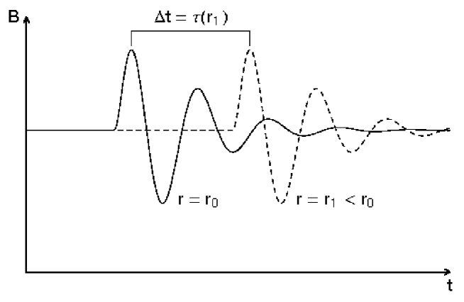
Figure 1: The retarded nature of the solution given by Eq. (44). A time variation in the magnetic field at radius $r_{0}$ will lead to the same variation in the magnetic field at radius $r_{1}<r_{0}$ at a later time, assuming the fluid moves toward smaller radii (i.e. toward the central black hole). The time delay is given by the time needed by a fluid particle moving from $r_{0}$ to $r_{1}$.

Eq. (44) gives a “retarded” solution to Eq. (43): at any time $t$ the solution at radius $r$ is given by the solution at an earlier time $t-\tau(r)$ at the radius $r_{0}$. Thus, a variation in the magnetic fields at any $r$ will propagate with the fluid motion (Fig. 1). The solution is unique if a suitable boundary or initial condition is imposed. For example, if a boundary condition is given on $t=0$: $\Psi(t=0,\tau)=\Psi_{1}(\tau)$, then the solution is $\Psi(t,\tau)=\Psi_{1}(\tau-t)$. In order for the solution to exist for a region specified by $t>0$ in the $t,\tau$-space, the boundary function $\Psi_{1}(\tau)$ must be defined on the whole $\tau$-axis: $-\infty<\tau<\infty$. Similarly, if a boundary condition is given on $\tau=0$ (i.e., $r=r_{0}$): $\Psi(t,\tau=0)=\Psi_{2}(t)$, then the solution is $\Psi(t,\tau)=\Psi_{2}(t-\tau)$. In this case, in order for the solution to exist for a region specified by $\tau>0$ in the $t,\tau$-space, the boundary function $\Psi_{2}(t)$ must be defined on the whole $t$-axis: $-\infty<t<\infty$.

We can also specify the boundary condition in another way

$$\Psi(t=0,\tau\geq 0)=\Psi_{1}(\tau)\;,\hskip 28.45274pt\Psi(t\geq 0,\tau=0)=\Psi_{2}(t)\;.$$ (45)

Then, the solution of Eq. (43) is

$$\Psi=\left\{\begin{array}[]{ll}\Psi_{1}(\tau-t)\;,&0\leq t\leq\tau\\ \Psi_{2}(t-\tau)\;,&0\leq\tau\leq t\end{array}\right.\;.$$ (48)

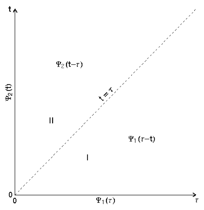
Figure 2: A sketch of the solution given by Eq. (48), corresponding to the boundary conditions given by Eq. (45). The parameter $\tau$ is defined by Eq. (42), which is the coordinate time needed by a particle moving from radius $r_{0}$ to radius $r$. So, $\tau=0$ corresponds to $r=r_{0}$, $\tau=\infty$ corresponds to the black hole horizon $r=r_{\rm H}$. The coordinate time is represented by $t$. In this diagram, the worldlines of fluid particles are represented by straight lines $t=\tau+{\rm constant}$. If the boundary conditions are imposed on the axes as shown in the diagram [Eq. (45)], the solution in the region between the $\tau$-axis and the dashed line $t=\tau$ (i.e., region I) is determined by the boundary condition on the $\tau$-axis, the solution in the region between the $t$-axis and the dashed line (i.e., region II) is determined by the boundary condition on the $t$-axis.

I.e., the value of $\Psi$ in region $0\leq t\leq\tau$ (region I) is determined by the value of $\Psi$ on the boundary $t=0,\tau\geq 0$; the value of $\Psi$ in region $0\leq\tau\leq t$ (region II) is determined by the value of $\Psi$ on the boundary $\tau=0,t\geq 0$ (see Fig. 2). In order for the solutions to be smoothly matched on the diagonal line $t=\tau\geq 0$ separating region I and region II, $\Psi_{1}(\tau)$ and $\Psi_{2}(t)$ must be smoothly matched at $t=\tau=0$:

$$\Psi_{1}(0)=\Psi_{2}(0)\;,\hskip 28.45274pt\left.\frac{d\Psi_{1}(\tau)}{d\tau}\right|_{\tau=0}=-\left.\frac{d\Psi_{2}(t)}{dt}\right|_{t=0}\;.$$ (49)

Given the solution of $\Psi$ in Eq. (44), we can solve $B^{r}$ from Eq. (41), then solve $B^{\phi}$ from Eq. (39). The results are

$$B^{r} = \frac{1}{r^{2}}(-C_{0}u_{t}+\Psi u_{\phi})\;,$$ (50a)

$$B^{\phi} = \frac{1}{r^{2}u^{r}}[-C_{0}u_{t}u^{\phi}+(1+u^{\phi}u_{\phi})\Psi]\;.$$ (50b)

Using Eq. (36), we obtain

$$B^{t}=\frac{1}{r^{2}u^{r}}[-(1+u^{t}u_{t})C_{0}+u^{t}u_{\phi}\Psi]\;.$$ (51)

Note that $B^{t}$, $B^{r}$, and $B^{\phi}$ satisfy the constraint Eq. (38), so among the three components only two are independent.

From Eqs. (32), (33), (50a), (50b), and the fact that $u_{t}=u_{a}(\partial/\partial t)^{a}=-E$ and $u_{\phi}=u_{a}(\partial/\partial\phi)^{a}=L$, we can solve for $B_{\hat{r}}$ and $B_{\hat{\phi}}$

$$B_{\hat{r}} = \frac{C_{0}E+\Psi L}{r\Delta^{1/2}}\;,$$ (52a)

$$B_{\hat{\phi}} = \frac{(C_{0}E+\Psi L)(\Omega-\omega v_{\hat{r}}^{2})\Gamma}{E\chi rv_{\hat{r}}}+\frac{\Psi}{Erv_{\hat{r}}}\;,$$ (52b)

where Eqs. (25) and (26) have been used to simplify the expression for $B_{\hat{\phi}}$. Since we focus on the solutions on the equatorial plane, here and hereafter we set $\Sigma=r^{2}$, and use $\chi$, $\omega$, and $A$ to refer their values at $\theta=\pi/2$. Note, in the solutions in Eqs. (50a) and (50b) [or, equivalently, Eqs. (52a) and (52b)] all the dependence on time $t$ is contained in the function $\Psi$.

Since we assume that the fluid particles move on geodesics, the specific angular momentum $L$ and the specific energy $E$ are constants. If $\Psi$ is also a constant, the combination $C_{0}E+\Psi L$ is a constant, which we denote as $C_{1}$. Then, Eqs. (52a) and (52b) become

$$B_{\hat{r}} = \frac{C_{1}}{r\Delta^{1/2}}\;,$$ (53a)

$$B_{\hat{\phi}} = \frac{C_{1}\Gamma(\Omega-\omega v_{\hat{r}}^{2})}{E\chi rv_{\hat{r}}}+\frac{\Psi}{Erv_{\hat{r}}}\;,$$ (53b)

which are stationary solutions of Maxwell’s equations.

If the black hole is a Schwarzschild black hole (i.e., the specific angular momentum $a=0$), the stationary solutions are reduced to

$$B_{\hat{r}} = \frac{C_{1}}{\chi r^{2}}\;,$$ (54a)

$$B_{\hat{\phi}} = \frac{C_{1}L}{Er^{3}v_{\hat{r}}}+\frac{\Psi}{Erv_{\hat{r}}}\;,$$ (54b)

where $E=\Gamma\chi$, $L=\Gamma\chi^{-1}\Omega r^{2}$, and $\chi^{2}=1-2M/r$. The non-stationary solutions can be obtained by replacing $C_{1}$ with $C_{0}E+\Psi L$.

V Evolution of magnetic fields in the plunging region

We are interested in the evolution of magnetic fields in the plunging region in the equatorial plane between $r=r_{\rm ms}$, the marginally stable circular orbit, and $r=r_{\rm H}$, the event horizon of the black hole.

For direct circular orbits (i.e., corotating with $L>0$) around a Kerr black hole, the radius of the marginally stable orbit is given by bar72

$$r_{\rm ms}=M\left\{3+z_{2}-\mathrm{sign}(a)\left[(3-z_{1})(3+z_{1}+2z_{2})\right]^{1/2}\right\}\;,$$ (55)

where $\mathrm{sign}(a)=1$ ($0,-1$) if $a>0$ ($=0,<0$), and

$$z_{1} \equiv 1+\left(1-\frac{a^{2}}{M^{2}}\right)^{1/3}\left[\left(1+\frac{a}{M}\right)^{1/3}+\left(1-\frac{a}{M}\right)^{1/3}\right]\;,$$ (56a)

$$z_{2} \equiv \left(z_{1}^{2}+3\frac{a^{2}}{M^{2}}\right)^{1/2}\;.$$ (56b)

The angular velocity of a particle geodesically moving on the marginally stable circular orbit is

$$\Omega_{\rm ms}=\left(\frac{M}{r_{\rm ms}^{3}}\right)^{1/2}\left[1+a\left(\frac{M}{r_{\rm ms}^{3}}\right)^{1/2}\right]^{-1}\;.$$ (57)

From Eqs. (24), (55-57), we can calculate the circular velocity on the marginally stable circular orbit by

$$v_{\hat{\phi},{\rm ms}}=\frac{A_{\rm ms}^{1/2}}{r_{\rm ms}\chi_{\rm ms}}\left(\Omega_{\rm ms}-\omega_{\rm ms}\right)\;,$$ (58)

the corresponding Lorentz factor by $\Gamma_{\rm ms}=(1-v_{\hat{\phi},{\rm ms}}^{2})^{-1/2}$, specific angular momentum $L_{\rm ms}$ by Eq. (25), and specific energy $E_{\rm ms}$ by Eq. (26) (setting $\theta=\pi/2$ and $r=r_{\rm ms}$). Here and hereafter the subscript “ms” represents the values at $r=r_{\rm ms}$.

Now let us choose the boundary radius $r_{0}=r_{\rm ms}$, the conserved specific angular momentum and specific energy to be

$$L=L_{\rm ms}(1-\delta)\;,\hskip 17.07182ptE=E_{\rm ms}\;,$$ (59)

where $0<\delta\ll 1$. I.e., we keep the specific energy the same as that on the marginally stable circular orbit, but decrease the specific angular momentum by a little amount. Then, we can calculate the Lorentz factor at $r=r_{\rm ms}$, corresponding to the specific energy and the specific energy specified by Eq. (59), by

$$\Gamma_{0}=\frac{1}{\chi_{\rm ms}}(E-L\omega_{\rm ms})\;;$$ (60)

and the corresponding boundary values of $v_{\hat{\phi}}$ and $v_{\hat{r}}$ at $r=r_{\rm ms}$ by

$$v_{\hat{\phi}0}=\frac{Lr_{\rm ms}}{\Gamma_{0}A_{\rm ms}^{1/2}}\;,\hskip 28.45274ptv_{\hat{r}0}=-\left(1-v_{\hat{\phi}0}^{2}-\frac{1}{\Gamma_{0}^{2}}\right)^{1/2}\;.$$ (61)

From Eqs. (25) and (26), we can calculate $\Gamma$, $\Omega$, $v_{\hat{\phi}}$, and $v_{\hat{r}}$ at any $r$ by

$$\Gamma = \frac{1}{\chi}(E-L\omega)\;,$$ (62a)

$$\Omega = \omega+\frac{L\chi^{2}r^{2}}{A(E-L\omega)}\;,$$ (62b)

$$v_{\hat{\phi}} = \frac{L\chi r}{A^{1/2}(E-L\omega)}\;,$$ (62c)

$$v_{\hat{r}} = -\left[1-\frac{\chi^{2}}{(E-L\omega)^{2}}\left(1+\frac{L^{2}r^{2}}{A}\right)\right]^{1/2}\;,$$ (62d)

where $E$ and $L$ are given by Eq. (59). The parameter $\tau$ defined by Eq. (42) can then be calculated with

$$\tau(r)=\int_{r_{\rm ms}}^{r}\frac{r}{\chi v_{\hat{r}}\Delta^{1/2}}\,dr\;.$$ (63)

With the above formulae at hands, we can calculate $B_{\hat{r}}$, $B_{\hat{\phi}}$, and $B^{2}=B_{\hat{r}}^{2}+B_{\hat{\phi}}^{2}-(B_{\hat{r}}v_{\hat{r}}+B_{\hat{\phi}}v_{\hat{\phi}})^{2}$ at any $r$ by Eqs. (52a) and (52b), giving the constant $C_{0}$ and the function $\Psi(t-\tau)$. To determine $C_{0}$ and $\Psi$, we need to specify the boundary conditions for the magnetic field. We will consider stationary solutions and non-stationary solutions separately.

V.1 Stationary solutions

It is straightforward to specify the boundary conditions for stationary solutions (i.e. solutions with $\Psi={\rm constant}$). To determine the solutions, we need only specify the values of $B_{\hat{r}}$ and $B_{\hat{\phi}}$ at $r=r_{\rm ms}$: $B_{\hat{r}0}$ and $B_{\hat{\phi}0}$. Then, by Eqs. (53a) and (53b), we have

$$C_{1} = B_{\hat{r}0}\chi_{\rm ms}A_{\rm ms}^{1/2}\;,$$ (64a)

$$\Psi = B_{\hat{\phi}0}Er_{\rm ms}v_{\hat{r}0}-B_{\hat{r}0}\Gamma_{0}A_{\rm ms}^{1/2}(\Omega_{0}-\omega_{\rm ms}v_{\hat{r}0}^{2})\;,$$ (64b)

where $C_{1}=C_{0}E+\Psi L$, $\Omega_{0}$ is the angular velocity corresponding to $v_{\hat{\phi}0}$

$$\Omega_{0}=\omega_{\rm ms}+\frac{v_{\hat{r}0}r_{\rm ms}\chi_{\rm ms}}{A_{\rm ms}^{1/2}}\;.$$ (65)

With the $C_{1}$ and $\Psi$ determined above, we can calculate $B_{\hat{r}}$, $B_{\hat{\phi}}$, and $B^{2}=B_{\hat{r}}^{2}+B_{\hat{\phi}}^{2}-(B_{\hat{r}}v_{\hat{r}}+B_{\hat{\phi}}v_{\hat{\phi}})^{2}$ at any $r$ by Eqs. (53a) and (53b). Since $B_{\hat{r}}$ and $B_{\hat{\phi}}$ linearly depend on $B_{\hat{r}0}$ and $B_{\hat{\phi}0}$, it is sufficient to study the effects of $B_{\hat{r}0}$ and $B_{\hat{\phi}0}$ separately. The results for any linear combination of $B_{\hat{r}0}$ and $B_{\hat{\phi}0}$ are simply linear superpositions of the results for $B_{\hat{r}0}$ and $B_{\hat{\phi}0}$ separately.

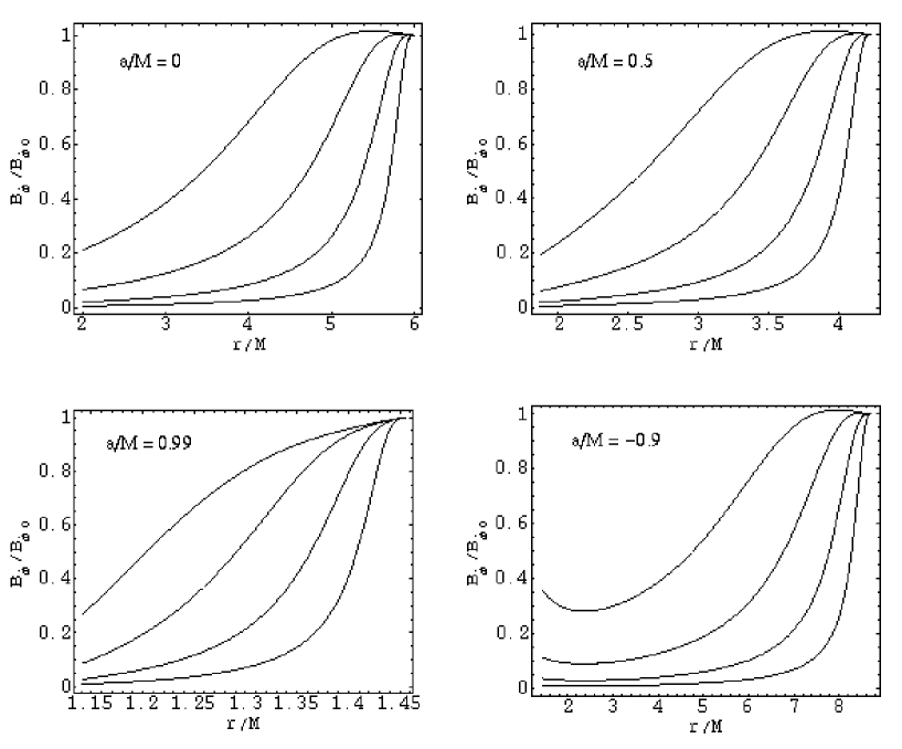
Figure 3: Stationary evolution of an initially toroidal magnetic field in the plunging region around a Kerr black hole. Each panel corresponds to a different spinning state of the black hole, as indicated by the dimensionless parameter $a/M$. Each curve starts from the marginally stable circular orbit ($r=r_{\rm ms}$, right end), ends at the horizon of the black hole ($r=r_{\rm H}$, left end). At $r=r_{\rm ms}$, the magnetic field is purely toroidal and has a value $B_{\hat{\phi}0}$, the fluid particles have specific energy identical to that of the marginally stable circular orbit, and specific angular momentum smaller than that of the marginally stable circular orbit by a tiny fraction $\delta$ [Eq. (59)]. In each panel, each curve corresponds to different values of $\delta$: $10^{-2}$, $10^{-3}$, $10^{-4}$ and $10^{-5}$ (downward). The radial component of the magnetic field is always zero.

In Fig. 3 we show the evolution results of $B_{\hat{\phi}}$ with the boundary condition $B_{\hat{\phi}}=B_{\hat{\phi}0}$ and $B_{\hat{r}}=0$ at $r=r_{\rm ms}$, for different spinning status of the black hole and different values of $\delta$ that specify the kinetic boundary conditions of the fluid. All quantities are scaled to the mass of the black hole so we do not need to specify the value of $M$. Since $B_{\hat{r}}$ does not depend on $B_{\hat{\phi}0}$, $B_{\hat{r}}$ is always zero. Since $C_{1}=0$ and $E={\rm constant}$, $B_{\hat{\phi}}$ evolves according to $B_{\hat{\phi}}\propto(rv_{\hat{r}})^{-1}$. Though in the plunging region $r$ decreases, $|v_{\hat{r}}|$ grows faster except at the neighbor of $r_{\rm ms}$. So the evolution of $B_{\hat{\phi}}$ is dominated by the variation of $v_{\hat{r}}$. Thus, as fluid particles get into the plunging region, $B_{\hat{\phi}}$ decreases quickly as clearly shown in Fig. 3. This radial expansion effect is not sensitive to the spin of the black hole, but very sensitive to the value of $\delta$ (or, effectively, the initial value of $v_{\hat{r}}$). As $\delta$ decreases (i.e., $|v_{\hat{r}0}|\propto\delta^{1/2}$ decreases), the fluid expands more as it gets into the plunging region, so the value of $B_{\hat{\phi}}$ decreases more.

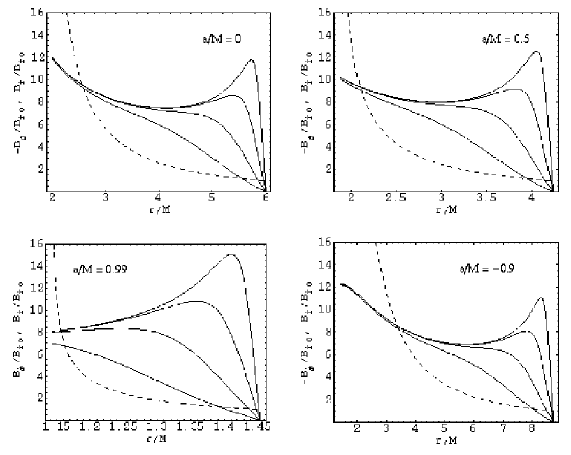
Figure 4: Similar to Fig. 3 but the magnetic field is initially radial, i.e. $B_{\hat{r}}=B_{\hat{r}0}$ and $B_{\hat{\phi}}=0$ at $r=r_{\rm ms}$. Solid lines represent the toroidal component of the magnetic field, dashed lines represent the radial component. Though initially the toroidal component of the magnetic field is zero, the shear motion of the fluid in the plunging region generates toroidal component from the radial component. The evolution of the radial component does not depend on the initial kinetic state of the fluid, so there is only one dashed line in each panel. The four solid lines representing the toroidal component of the magnetic field correspond to different values of $\delta$: $10^{-2}$, $10^{-3}$, $10^{-4}$ and $10^{-5}$ (upward).

In Fig. 4 we show the evolution results of $B_{\hat{r}}$ (dashed lines) and $B_{\hat{\phi}}$ (solid lines) with the boundary condition $B_{\hat{r}}=B_{\hat{r}0}$ and $B_{\hat{\phi}}=0$ at $r=r_{\rm ms}$. Though at $r=r_{\rm ms}$ we have $B_{\hat{\phi}}=0$, in the plunging region $B_{\hat{\phi}}$ becomes nonzero since $B_{\hat{\phi}}$ depends on both $B_{\hat{r}0}$ and $B_{\hat{\phi}0}$ [Eqs. (53b), (64a) and (64b)]. This is the manifestation that the shear motion of the fluid in the plunging region generates $B_{\hat{\phi}}$ from $B_{\hat{r}}$. The radial component of the magnetic field, $B_{\hat{r}}$, increases gradually as the fluid enters the plunging region, according to $B_{\hat{r}}\propto(r\Delta^{1/2})^{-1}$, and blows up on the black hole horizon where $\Delta=0$. The shear motion of the fluid does not amplify $B_{\hat{r}}$, which echos with the fact that $B_{\hat{r}}$ is always zero if it is zero at $r=r_{\rm ms}$ (Fig. 3). Since $B_{\hat{r}}$ does not depend on $v_{\hat{r}}$, there is only one dashed line in each panel of Fig. 4. In comparison, the toroidal component, $B_{\hat{\phi}}$, increases more quickly in the transition region, since the shear motion of the fluid magnifies $B_{\hat{\phi}}$. This is more prominent for small values of $\delta$ (i.e. small $|v_{\hat{r}0}|$), since $B_{\hat{\phi}}\propto v_{\hat{r}}^{-1}$ [Eq. (53b)] and $v_{\hat{r}}$ is close to $v_{\hat{r}0}$ as the particles just leave the marginally stable circular orbit. For small values of $\delta$, $B_{\hat{\phi}}$ increases sharply as the fluid just gets into the plunging region, then decreases a little bit due to the radial expansion of the fluid. Unlike $B_{\hat{r}}$, $B_{\hat{\phi}}$ is always finite on the black hole horizon. We see that, $B_{\hat{r}}$ and $B_{\hat{\phi}}$ evolves in very different ways.

From Fig. 4 we also see that the evolution of the magnetic field in the plunging region depends on the spin of the black hole, though not very sensitively. Interestingly, the toroidal component and the poloidal component depend on the spin of the black hole in an opposite way. As the dimensionless spin parameter $a/M$ increases from zero to positive values, the shear amplification effect on the toroidal component of the magnetic field increases (except for the case of $\delta=10^{-2}$ for which the amplification effect is not prominent), while the amplification of the radial component caused by the compression in the azimuthal direction (i.e., the decrease in radius $r$) decreases. But, if $a/M$ decreases from zero to negative values, the shear amplification effect on the toroidal component of the magnetic field decreases, while the compression amplification of the radial component increases. The opposite dependence for positive and negative spins is probably due to the different coordinate distances from the marginally stable circular orbit to the black hole horizon for black holes of positive and negative spins.

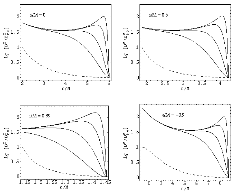
Figure 5: Stationary evolution of $B^{2}=B_{a}B^{a}$ (solid curves). The boundary conditions are the same as that in Fig. 4. The thin dashed line in each panel shows the absolute value of the radial velocity (i.e. $|v_{\hat{r}}|$) of the fluid, corresponding to $\delta=10^{-5}$. If we choose a different value of $\delta$, the curve for the radial velocity will change slightly: the right end will change according to $|v_{\hat{r}}|\propto\delta^{1/2}$, the left end always approaches $1$ (i.e. the speed of light). (For brevity, $\lg\left[B^{2}/B_{\hat{r}0}^{2}\right]$ and $|v_{\hat{r}}|$ use the same scale as labeled on the left side of the box in each panel.)

In Fig. 5 we show the evolution of $B^{2}$ [defined by Eq. (28)] with the same boundary conditions in Fig. 4. As the fluid just enters the plunging region (near the right ends of curves), $B^{2}$ sharply increases due to the small values of $|v_{\hat{r}}|$ there, which is the manifestation of amplification effect caused by the shear rotation of the fluid. After that, i.e., after the fluid obtains a large radial velocity (the dashed lines in the figure), the amplification effect is reduced but the expansion effect becomes prominent [see Eq. (13)]. On the horizon of the black hole $B^{2}$ is always finite, so the boundary conditions on the horizon is satisfied (tho86, , and references therein).

V.2 Non-stationary solutions

To specify the boundary conditions for non-stationary solutions is a little bit complicated. As discussed earlier, to determine the solutions in a region with $t>0$ and $\tau>0$ (i.e. $r_{\rm H}<r<r_{\rm ms}$) in the $t,\tau$-space, we need to specify the boundary conditions on the axes ($t=0,\tau\geq 0$) and ($t\geq 0,\tau=0$), i.e. specify $\Psi_{1}(\tau)$ and $\Psi_{2}(t)$ [see Eq. (45)].

As an example, let us assume that $\Psi_{2}(t)={\rm constant}$, and $B_{\hat{\phi}}=0$ on the axis ($t=0,\tau\geq 0$). I.e., the solution on the boundary $\tau=0$ is stationary for $t\geq 0$, and the $\hat{\phi}$-component of the magnetic field in the plunging region is zero at $t=0$. Equivalently, we specify the boundary conditions as follows:

$${\rm On}\;\,r=r_{\rm ms},\;t\geq 0:\hskip 41.34193ptB_{\hat{r}}=B_{\hat{r}0},\;\;B_{\hat{\phi}}=0\;;$$ (66a)

$${\rm On}\;\,t=0,\;r_{\rm H}<r<r_{\rm ms}:\hskip 14.22636ptB_{\hat{\phi}}=0\;.\hskip 60.3197pt$$ (66b)

Then, if we apply Eqs. (52a) and (52b) to the boundary at $r=r_{\rm ms}$ and $t\geq 0$, we can solve for $C_{0}$ and $\Psi_{2}$. The results are

$$C_{0} = \frac{B_{\hat{r}0}A_{\rm ms}^{1/2}}{E}\left[(\Omega_{0}-\omega_{\rm ms}v_{\hat{r}0}^{2})L\Gamma_{0}+\chi_{\rm ms}\right]\;,$$ (67a)

$$\Psi_{2} = -\Gamma_{0}B_{\hat{r}0}A_{\rm ms}^{1/2}(\Omega_{0}-\omega_{\rm ms}v_{\hat{r}0}^{2})\;.$$ (67b)

Applying Eq. (52b) to the boundary at $t=0$ and $r_{\rm H}<r<r_{\rm ms}$, and substituting Eq. (67a) for $C_{0}$, we can solve for $\Psi_{1}$

$$\Psi_{1}(\tau)=\Psi_{1}[r(\tau)]\;,\hskip 28.45274pt\Psi_{1}(r)=\frac{(\Omega-\omega v_{\hat{r}}^{2})\Gamma EC_{0}}{(\Omega-\omega v_{\hat{r}}^{2})\Gamma L+\chi}\;,$$ (68)

where $r(\tau)$ is given by the inverse of $\tau(r)$. The values of $B_{\hat{r}}$ on $t=0$ and $r_{\rm H}<r<r_{\rm ms}$ is then determined by Eq. (52a).

With the $\Psi_{1}$ and $\Psi_{2}$ determined above, we can obtain $\Psi$ by Eq. (48). This, together with the $C_{0}$ given by Eq. (67a), allows us to calculate $B_{\hat{r}}$ and $B_{\hat{\phi}}$ with Eqs. (52a) and (52b) for any radius in the plunging region at any time $t>0$.

It is easy to check that $\Psi_{1}(\tau=0)=\Psi_{2}$, so the solutions are continuously matched on the line $t=\tau$. Since

$$\frac{d\Psi_{1}(\tau)}{d\tau}=\frac{d\Psi_{1}(r)}{dr}\,\frac{dr}{d\tau}=\frac{d\Psi_{1}(r)}{dr}\,\frac{\chi v_{\hat{r}}\Delta^{1/2}}{r}\;,$$ (69)

the solutions are smoothly matched on the line $t=\tau$ only in the limit $v_{\hat{r}0}=0$ since then we have $d\Psi_{1}/d\tau=0=-d\Psi_{2}/dt$ at $\tau=t=0$. If $v_{\hat{r}0}$ is not zero but small ($|v_{\hat{r}0}|\ll 1$), the solutions are approximately smoothly matched on the line $t=\tau$ if $|d\Psi_{1}(r)/dr|$ is not large at $r=r_{\rm ms}$.

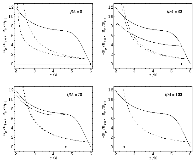
Figure 6: Time evolution of magnetic fields around a Schwarzschild black hole (i.e. $a=0$). Each panel corresponds to a particular moment. Thick solid lines show the toroidal component of the magnetic field (i.e., $B_{\hat{\phi}}$), thick dashed lines show the radial component (i.e., $B_{\hat{r}}$). The thin (upper) lines show the corresponding stationary state solutions. The fluid particles have specific energy identical to that of the marginally stable circular orbit, and specific angular momentum smaller than that of the marginally stable circular orbit by a factor of $\delta=10^{-3}$. The first (left and up) panel shows the initial and boundary conditions of the magnetic field: on $r=r_{\rm ms}$ (right end), $B_{\hat{\phi}}=0$, $B_{\hat{r}}=B_{\hat{r}0}$ for all time $t>0$; in the plunging region ($r_{\rm H}<r<r_{\rm ms}$), $B_{\hat{\phi}}=0$ at $t=0$ [i.e., Eqs. (66a) and (66b); the corresponding $B_{\hat{r}}$ at $t=0$ is automatically determined by the solutions]. The figures show that, as time goes on, the magnetic field quickly approaches and saturates at the state given by the stationary solutions. The black dot in each panel shows the radial position of a fluid particle at each moment: initially the particle is at $r=r_{\rm ms}$.

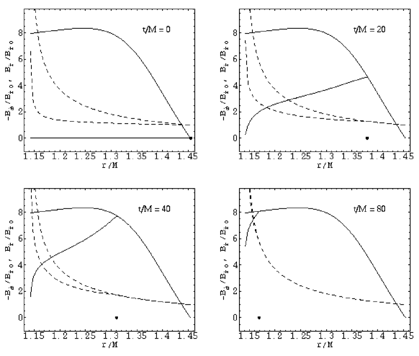
Figure 7: Same as Fig. 6 but for a Kerr black hole with $a/M=0.99$.

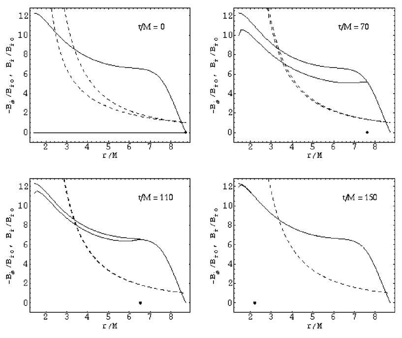
Figure 8: Same as Figs. 6 and 7 but for a Kerr black hole with $a/M=-0.9$.

In Figs. 6 – 8 we show the results for the non-stationary evolution of magnetic fields. Each figure corresponds to a different spinning state of the black hole. In Fig. 6 $a/M=0$, in Fig. 7 $a/M=0.99$, while in Fig. 8 $a/M=-0.9$. The boundary conditions for the magnetic field are given by Eqs. (66a) and (66b). The kinetic boundary conditions of the fluid are given by Eq. (59), here we assume $\delta=10^{-3}$. In each figure, each panel corresponds to the state of the magnetic field at a particular moment. Especially, the first (left and up) panel shows the initial ($t=0$) state of the magnetic field [i.e. Eqs. (66a) and (66b)]. In each panel, the thick dashed line shows $B_{\hat{r}}$, the thick solid line shows $B_{\hat{\phi}}$, and the thin lines show the corresponding stationary solutions. Each curve starts from the marginally stable circular orbit (right end) and ends on the horizon of the black hole (left end).

From these figures we see that, though initially the magnetic field is deviated from the stationary state, it evolves to and finally saturates at the stationary state as time goes on. Since we hold the magnetic field on the marginally stable circular orbit in a stationary state for $t\geq 0$ [Eq. (66a)] and the fluid moves from the marginally stable circular orbit toward the horizon of the black hole, the stationary state propagates from the marginally stable circular orbit toward the horizon of the black hole (i.e., from right to left in the figures). This is clear seen in Figs. 6 – 8: the magnetic field at a radius closer to the right end of the curve gets into the stationary state earlier. In each panel, with a black dot we show the position of a particle that is at the marginally stable radius at $t=0$, which clearly shows the propagation of the state of the magnetic field with the motion of the fluid. This suggests that the stationary state of the magnetic field in the plunging region is uniquely determined by the boundary conditions at the marginally stable circular orbit.

The figures also show the dependence of the evolution of the magnetic field on the spin of the black hole. For a black hole with a negative $a$ a longer coordinate time is needed for most of the fluid in the plunging region to settle into the stationary state. This is apparently caused by the fact that a black hole with a negative $a$ has a larger coordinate radial distance from the marginally stable circular orbit to the horizon.

VI Can magnetic fields become dynamically important in the plunging region?

In previous sections we have studied the evolution of magnetic fields in the plunging region and seen that magnetic fields can be amplified by the convergence (the radial magnetic field) and shear motion (the toroidal magnetic field) of the fluid. Thus, we can ask if magnetic fields can become dynamically important in the plunging region assuming that their dynamical effects are negligible at the marginally stable circular orbit. We try to answer this question in this section.

VI.1 Dynamical effects of the magnetic field

Assuming that in the plunging region the gas pressure of the fluid is negligible, then the total stress-energy tensor of the fluid is

$$T^{ab}=\rho_{\rm m}u^{a}u^{b}+T_{\rm EM}^{ab}\;,$$ (70)

where $\rho_{\rm m}$ is the mass-energy density of the fluid matter measured by an observer comoving with the fluid, $T_{\rm EM}^{ab}$ is the stress-energy tensor of the electromagnetic field as given by Eq. (5). Then, the equation of motion of the fluid is given by

$$\nabla_{a}T^{ab}=\rho_{\rm m}u^{a}\nabla_{a}u^{b}+u^{b}\nabla_{a}(\rho_{\rm m}u^{a})+\nabla_{a}T_{\rm EM}^{ab}=0\;.$$ (71)

When Maxwell’s equations are satisfied we have $\nabla_{a}T_{\rm EM}^{ab}=-F^{ab}J_{b}$ mis73 . Then, by Eq. (2), we have $u_{b}\nabla_{a}T_{\rm EM}^{ab}=0$ for a magnetic field frozen to the fluid. Therefore, the contraction of $u_{b}$ with Eq. (71) leads to the equation of continuity

$$\nabla_{a}J_{\rm m}^{a}=0\;,\hskip 28.45274ptJ_{\rm m}^{a}\equiv\rho_{\rm m}u^{a}\;,$$ (72)

where $J_{\rm m}^{a}$ is the flux density vector of mass. The equation of continuity does not explicitly contain magnetic field variables. Since $(\partial/\partial t)^{a}$ and $(\partial/\partial\phi)^{a}$ are Killing vectors, Eq. (71) leads to the conservation of angular momentum and energy

$$\nabla_{a}J_{\rm L}^{a}=0\;,\hskip 28.45274pt\nabla_{a}J_{\rm E}^{a}=0\;,$$ (73)

where

$$J_{\rm L}^{a}\equiv\left(\frac{\partial}{\partial\phi}\right)^{b}T_{b}^{\,\,a}=\left(\rho_{\rm m}+\frac{1}{4\pi}B^{2}\right)Lu^{a}-\frac{1}{4\pi}B_{\phi}B^{a}$$ (74)

is the flux density vector of angular momentum,

$$J_{\rm E}^{a}\equiv-\left(\frac{\partial}{\partial t}\right)^{b}T_{b}^{\,\,a}=\left(\rho_{\rm m}+\frac{1}{4\pi}B^{2}\right)Eu^{a}+\frac{1}{4\pi}B_{t}B^{a}$$ (75)

is the flux density vector of energy.

Here we look for stationary and axisymmetric solutions in the plunging region. Then, with the assumptions adopted in this paper, i.e. $\partial/\partial t=\partial/\partial\phi=0$, $u^{\theta}=B^{\theta}=0$ and $\partial u^{\theta}/\partial\theta=\partial B^{\theta}/\partial\theta=0$, in the equatorial plane the equation of continuity is reduced to

$$\frac{d}{dr}\left(r^{2}\rho_{\rm m}u^{r}\right)=0\;.$$ (76)

Similarly, the equations of angular momentum and energy conservation are reduced to

$$\frac{d}{dr}\left\{r^{2}\left[\left(\rho_{\rm m}+\frac{1}{4\pi}B^{2}\right)Lu^{r}-\frac{1}{4\pi}B_{\phi}B^{r}\right]\right\}=0\;,$$ (77)

and

$$\frac{d}{dr}\left\{r^{2}\left[\left(\rho_{\rm m}+\frac{1}{4\pi}B^{2}\right)Eu^{r}+\frac{1}{4\pi}B_{t}B^{r}\right]\right\}=0\;.$$ (78)

The solution of Eq. (76) is

$$\rho_{\rm m}=\frac{F_{\rm m}}{4\pi r^{2}u^{r}}=\frac{F_{\rm m}}{4\pi\Gamma\chi A^{1/2}v_{\hat{r}}}\;,$$ (79)

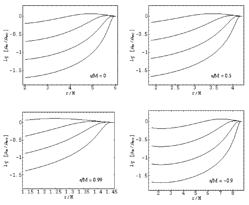
Figure 9: Stationary evolution of the mass density in the plunging region around a Kerr black hole. Each panel corresponds to a different spinning state of the black hole, as indicated by the values of $a/M$. The right end of each curve corresponds to the marginally stable circular orbit ($r=r_{\rm sm}$). The left end of each curve corresponds to the horizon of the black hole ($r=r_{\rm H}$). The kinetic boundary conditions are given by Eq. (59). In each panel the four curves correspond respectively to $\delta=10^{-2}$, $10^{-3}$, $10^{-4}$ and $10^{-5}$ (downward). The mass density is in units of $\rho_{{\rm m}0}$ – the mass density at the marginally stable circular orbit.

where $F_{\rm m}=4\pi r^{2}J_{\rm m}^{r}$ is a constant to be determined by the boundary conditions, which measures the mass flux across radius $r$. Fig. 9 shows the variation of the mass density with radius in the plunging region, assuming that fluid particles move on geodesics. The kinetic boundary conditions are given by Eq. (59). In each panel (corresponding to a different spinning state of the black hole), we show the ratio of $\rho_{\rm m}/\rho_{{\rm m}0}$ corresponding to four different values of $\delta$: $10^{-2}$, $10^{-3}$, $10^{-4}$ and $10^{-5}$, where $\rho_{{\rm m}0}\equiv\rho(r=r_{\rm ms})$. We see that, the evolution of the mass density of the fluid sensitively depends on the value of $\delta$ (or effectively, the value of $|v_{\hat{r}0}|\propto\delta^{1/2}$). While for not very small $\delta$ (e.g., $\delta=10^{-2}$) the variation of $\rho_{\rm m}$ is not dramatic, for very small $\delta$ (e.g., $\delta=10^{-5}$) the variation of $\rho_{\rm m}$ is dramatic: as the fluid gets into the plunging region the mass density drops sharply. This is caused by the sharp increase in the ratio $v_{\hat{r}}/v_{\hat{r}0}$ in the plunging region for small $\delta$.

From Eqs. (77) and (78) we see that the dynamical role played by the magnetic field is characterized by the following three dimensionless parameters

$$\eta_{1}\equiv\frac{B^{2}}{4\pi\rho_{\rm m}}\;,\hskip 28.45274pt\eta_{2}\equiv\left|\frac{B_{\phi}B^{r}}{4\pi\rho_{\rm m}Lu^{r}}\right|\;,\hskip 28.45274pt\eta_{3}\equiv\left|\frac{B_{t}B^{r}}{4\pi\rho_{\rm m}Eu^{r}}\right|\;.$$ (80)

The parameter $\eta_{1}$ measures the transfer of angular momentum and energy from the fluid particles to the magnetic field; $\eta_{2}$ and $\eta_{3}$ measure the transportation of angular momentum and energy from one part to another by the magnetic tension in the rest frame of the fluid. To justify the assumption that the effects of the magnetic field on the dynamics of the fluid particles are negligible, we must require that

$$\eta_{1}\ll 1\;,\hskip 28.45274pt\eta_{2}\ll 1\;,\hskip 28.45274pt\eta_{3}\ll 1\;.$$ (81)

In Eq. (80), $\rho_{\rm m}$ is given by Eq. (79), $B^{2}$ is calculated by Eq. (28) (setting $v_{\hat{\theta}}=B_{\hat{\theta}}=0$), $B_{\phi}B^{r}$ and $B_{t}B^{r}$ are calculated by

$$B_{\phi}B^{r}=\frac{\chi A}{r^{3}}B_{\hat{r}}B_{\hat{\phi}}\;,\hskip 28.45274ptB_{t}B^{r}=-\frac{\chi A^{1/2}}{r^{3}}B_{\hat{r}}\left(\chi rB_{\hat{r}}v_{\hat{r}}+A^{1/2}B_{\hat{\phi}}\Omega\right)\;.$$ (82)

Near the marginally stable circular orbit, we have $|v_{\hat{r}}/v_{\hat{\phi}}|\ll 1$, $E\geq L\Omega$, and $B_{t}B^{r}\approx-\Omega B_{\phi}B^{r}$. Therefore, from the definitions of $\eta_{2}$ and $\eta_{3}$, we have

$$\eta_{3}\approx\frac{\Omega L}{E}\eta_{2}\leq\eta_{2}\;,$$ (83)

at $r\approx r_{\rm ms}$.

From Fig. 9 we see that for small $\delta$ the mass density $\rho_{\rm m}$ drops quickly as the fluid enters the plunging region. However, the evolution of $B^{2}$ in the plunging region sensitively depends on the orientation of the magnetic field on the marginally stable circular orbit. From Fig. 5, the value of $B^{2}$ corresponding to an initially radial magnetic field increases as the fluid enters the plunging region, because of the convergence of the radial magnetic field and the shear amplification of the toroidal magnetic field. If the initial magnetic field is purely toroidal, on the other hand, from Fig. 3 we see that the magnetic field keeps purely toroidal in the plunging region and the dilution effect arising from the drop in the mass density makes $B_{\hat{\phi}}$ (and thus $B^{2}$) decrease in the plunging region. Therefore, in the plunging region the variation of $\eta_{1}$, $\eta_{2}$, and $\eta_{3}$ sensitively depends on the boundary condition of the magnetic field on the marginally stable circular orbit. We can imagine that, if on the marginally stable circular orbit the magnetic field is purely radial, then in the plunging region $B^{2}$ increases so the ratio $\eta_{1}$ also increases as $\rho_{\rm m}$ decreases. In such a case, $\eta_{1}$ may become close to or even greater than $1$ in the plunging region even if it is $\ll 1$ on the marginally stable circular orbit, then the dynamical effects of the magnetic field become important in the plunging region. On the other hand, if on the marginally stable circular orbit the magnetic field is purely toroidal, then in the plunging region $B^{2}$ decreases which causes $\eta_{1}$ to decrease also if $B^{2}$ decreases faster than $\rho_{\rm m}$. Therefore, to correctly estimate the dynamical effects of magnetic fields in the plunging region, we must choose a sensible boundary condition for the magnetic field on the marginally stable circular orbit.

The magnetic field on the marginally stable circular orbit is determined by the MHD processes in the disk region. In the disk region ($r>r_{\rm ms}$), particles move on nearly circular orbits with $|v_{\hat{r}}|\ll|v_{\hat{\phi}}|$. As a disk particle moves a finite distance in the radial direction, it has undergone an infinite number ($\gg 1$) of turns around the central black hole. As a result, the magnetic field lines frozen to the fluid are wound up around the center an infinite number of times. Therefore, in a stationary state, we expect that the magnetic field in the disk region is predominantly toroidal. In the Appendix we solve Maxwell’s equations in the disk region and show that in the stationary state the magnetic field in the disk is likely to be parallel to the velocity field: $B^{\phi}/B^{r}=u^{\phi}/u^{r}$. Thus, in the stationary state, on the marginally stable circular orbit the magnetic field does not take any orientation but the one that satisfies the following condition

$$\frac{B^{\phi}u^{r}}{B^{r}u^{\phi}}=1\;.$$ (84)

On the marginally stable circular orbit, Eq. (84) implies that $|B_{\hat{r}}|\ll|B_{\hat{\phi}}|$ since $|v_{\hat{r}}|\ll|v_{\hat{\phi}}|$.

From Eqs. (50a) and (50b), we have

$$\frac{B^{\phi}u^{r}}{B^{r}u^{\phi}}=1+\frac{\Psi}{(-C_{0}u_{t}+\Psi u_{\phi})u^{\phi}}\;.$$ (85)

Then, Eq. (84) is satisfied if and only if $\Psi=0$ on the marginally stable circular orbit. In the stationary state $\Psi$ is a constant, so we have

$$\Psi=0$$ (86)

throughout the plunging region. Thus, in the stationary state, Eq. (84) holds throughout the plunging region .

Inserting Eqs. (32) and (33) into Eq. (84), we obtain

$$\frac{B_{\hat{r}}}{B_{\hat{\phi}}}=\frac{Erv_{\hat{r}}}{\Gamma A^{1/2}(\Omega-\omega v_{\hat{r}}^{2})}\;.$$ (87)

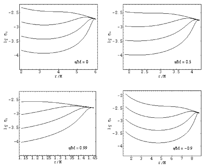
Figure 10: Stationary evolution of the ratio $\eta_{1}\equiv B^{2}/4\pi\rho_{\rm m}$ in the plunging region. Each panel corresponds to a different spinning state of the black hole, as indicated by the values of $a/M$. The kinetic boundary conditions are given by Eq. (59). The boundary conditions for the magnetic field are: on $r=r_{\rm ms}$ we have $B_{\hat{\phi}}=0.05$ in units of $(4\pi\rho_{{\rm m}0})^{1/2}$. The corresponding $B_{\hat{r}}$ is calculated with Eq. (87) so that the magnetic field is always parallel to the velocity field. In each panel the four curves correspond respectively to $\delta=10^{-2}$, $10^{-3}$, $10^{-4}$ and $10^{-5}$ (downward). Each curve starts from the marginal stable circular orbit (right end) and ends at the horizon of the black hole (left end).

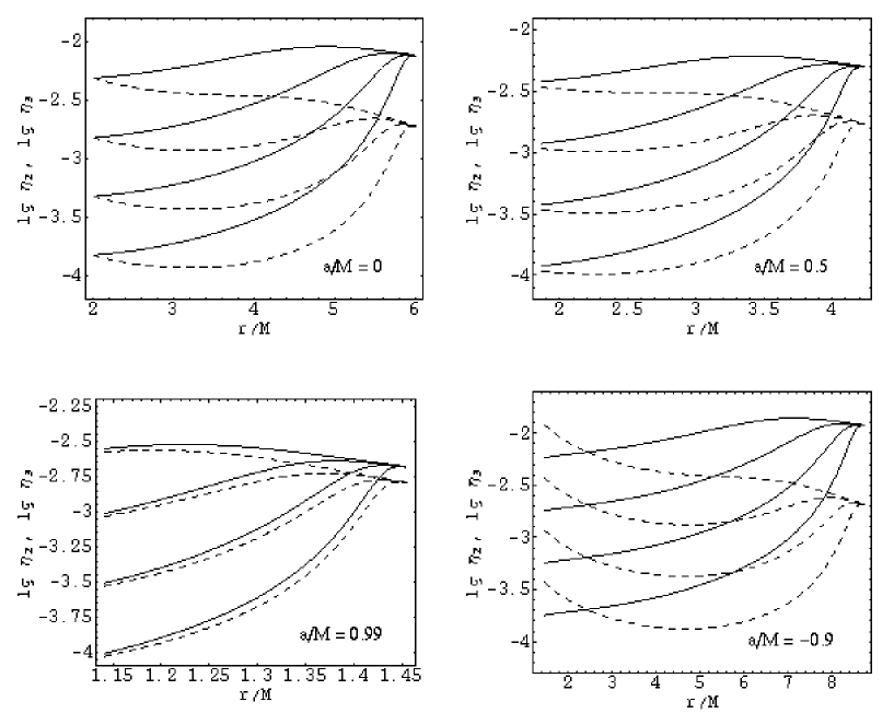
Figure 11: Same as Fig. 10 but for the ratios $\eta_{2}\equiv\left|B_{\phi}B^{r}/(4\pi\rho_{\rm m}Lu^{r})\right|$ (solid curves) and $\eta_{3}\equiv\left|B_{t}B^{r}/(4\pi\rho_{\rm m}Eu^{r})\right|$ (dashed curves).

We have calculated $\eta_{1}$, $\eta_{2}$, and $\eta_{3}$ in the plunging region, assuming that they all are $\ll 1$ at $r=r_{\rm ms}$ and the boundary condition (86) is satisfied. At $r=r_{\rm ms}$ the toroidal magnetic field is assumed to be $B_{\hat{\phi}}=0.05$ in units of $(4\pi\rho_{\rm m})^{1/2}$, the corresponding radial magnetic field $B_{\hat{r}}$ is then given by Eq. (87). The parameter $\delta$ is taken to be $10^{-2}$, $10^{-3}$, $10^{-4}$ and $10^{-5}$, alternatively. The results are shown in Figs. 10 and 11. From these figures we see that, in the plunging region the evolution of $\eta_{1}$, $\eta_{2}$ and $\eta_{3}$ sensitively depends on the value of $\delta$. For very small $\delta$, $\eta_{1}$, $\eta_{2}$ and $\eta_{3}$ quickly decrease as the fluid gets into the plunging region. This is caused by the fact that a very small $\delta$ (i.e., a very small $|v_{\hat{r}0}|\propto\delta^{1/2}$) corresponds to a very small $|B_{\hat{r}0}|$ according to the boundary condition (84), while the magnetic field in the plunging region is predominantly determined by $|B_{\hat{r}0}|$ instead of $|B_{\hat{\phi}0}|$ (see Figs. 3 and 4). For a moderate $\delta$ (e.g., $\delta=10^{-2}$), $\eta_{1}$, $\eta_{2}$ and $\eta_{3}$ may increase in the plunging region. However, even in this case, the conditions in Eq. (81) are always satisfied throughout the plunging region.

VI.2 Self-consistent solutions to the dynamical equations

If we insert the solutions of Maxwell’s equations that we obtained in Sec. IV into Eqs. (77) and (78), then apply Eq. (79), we obtain

$$\frac{d}{dr}\left(F_{\rm m}L+4\pi r^{2}\,T_{{\rm EM},\phi}^{~{}~{}~{}~{}~{}r}\right) = 0\;,$$ (88)

$$\frac{d}{dr}\left(F_{\rm m}E-4\pi r^{2}\,T_{{\rm EM},t}^{~{}~{}~{}~{}~{}r}\right) = 0\;,$$ (89)

where

$$T_{{\rm EM},\phi}^{~{}~{}~{}~{}~{}r}=-\frac{C_{0}\Delta}{4\pi r^{4}u^{r}}\left(C_{0}u^{\phi}+\Psi u^{t}\right)\;,\hskip 28.45274ptT_{{\rm EM},t}^{~{}~{}~{}~{}~{}r}=\frac{\Psi}{C_{0}}T_{{\rm EM},\phi}^{~{}~{}~{}~{}~{}r}\;.$$ (90)

When $\Psi=0$ [i.e., Eq. (84) is satisfied in the plunging region], we have $T_{{\rm EM},t}^{~{}~{}~{}~{}~{}r}=0$. Then Eq. (89) implies that $E$ keeps constant in the plunging region. However, since $T_{{\rm EM},\phi}^{~{}~{}~{}~{}~{}r}\neq 0$, by Eq. (88) $L$ varies in the plunging region. Therefore, for the solutions satisfying the boundary condition (84) [or, equivalently, Eq. (86)], the specific energy of particles is conserved but the specific angular momentum changes.

Setting $L=u_{\phi}$, $E=-u_{t}$, and $\Psi=0$, Eqs. (88) and (89) can be integrated to obtain

$$u_{\phi}+\frac{c_{0}^{2}\Delta u^{\phi}}{r^{2}u^{r}} = -f_{\rm L}\;,$$ (91)

$$u_{t} = f_{\rm E}\;,$$ (92)

where

$$c_{0}\equiv\frac{C_{0}}{\sqrt{-F_{\rm m}}}\;,\hskip 28.45274ptf_{\rm L}\equiv\frac{F_{\rm L}}{-F_{\rm m}}\;,\hskip 28.45274ptf_{\rm E}\equiv\frac{F_{\rm E}}{-F_{\rm m}}\;,$$ (93)

where $F_{\rm L}=4\pi r^{2}J_{\rm L}^{r}$ and $F_{\rm E}=4\pi r^{2}J_{\rm E}^{r}$ are constants measuring the angular momentum flux and the energy flux across radius $r$, respectively. Using $u^{\phi}=g^{\phi\phi}u_{\phi}+g^{\phi t}u_{t}$, we can solve Eqs. (91) and (92) for $u_{\phi}$

$$u_{\phi}=\frac{\frac{2Mac_{0}^{2}}{r^{3}u^{r}}f_{\rm E}-f_{\rm L}}{1+\frac{c_{0}^{2}}{r^{2}u^{r}}\left(1-\frac{2M}{r}\right)}\;.$$ (94)

Then, from $g^{ab}u_{a}u_{b}=-1$ and $u_{r}=g_{rr}u^{r}$, we obtain the equation for $u^{r}$

$$\left(ru^{r}\right)^{2}=-\Delta\left(1-\frac{f_{\rm E}^{2}}{1-\frac{2M}{r}}\right)-\frac{1}{1-\frac{2M}{r}}\left[\frac{\frac{2Ma}{r}f_{\rm E}+\left(1-\frac{2M}{r}\right)f_{\rm L}}{1+\frac{c_{0}^{2}}{r^{2}u^{r}}\left(1-\frac{2M}{r}\right)}\right]^{2}\;.$$ (95)

Though the factor $\left(1-\frac{2M}{r}\right)$ appears in the denominators on the right-hand side of Eq. (95), $r=2M$ is not a singularity of the equation, since the factor $\left(1-\frac{2M}{r}\right)$ disappears from the denominators if we expand the second term on the right-hand side of Eq. (95), then combine with the first term. However, the factor $\left[1+\frac{c_{0}^{2}}{r^{2}u^{r}}\left(1-\frac{2M}{r}\right)\right]$ represents a singularity of Eq. (95) at

$$1+\frac{c_{0}^{2}}{r^{2}u^{r}}\left(1-\frac{2M}{r}\right)=0\;.$$ (96)

The differentiation of Eq. (95) with respect to $u^{r}$ gives rise to another singularity of the equation, which is at

$$u_{r}u^{r}-\frac{c_{0}^{2}}{r^{2}u^{r}}\left(1-\frac{2M}{r}-f_{\rm E}^{2}\right)=0\;.$$ (97)

This singularity appears as one differentiates Eq. (95) with respect to $r$ to obtain a differential equation for $u^{r}$.

If we define the relativistic Alfvén velocity by

$$c_{\rm A}^{~{}\,a}\equiv\frac{B^{a}}{\sqrt{4\pi\rho_{\rm m}+B^{2}}}\;,$$ (98)

then we have

$$1+\frac{c_{0}^{2}}{r^{2}u^{r}}\left(1-\frac{2M}{r}\right)=\frac{1}{1-c_{\rm A}^{2}}\left(1-\frac{c_{{\rm A}r}c_{\rm A}^{~{}\,r}}{u_{r}u^{r}}\right)\;,$$ (99)

and

$$\frac{c_{0}^{2}}{r^{2}u^{r}}\left(1-\frac{2M}{r}-f_{\rm E}^{2}\right)=\frac{c_{\rm A}^{2}}{1-c_{\rm A}^{2}}\;,$$ (100)

where $c_{\rm A}^{2}\equiv c_{{\rm A}a}c_{\rm A}^{~{}\,a}<1$. Therefore, the singularities given by Eqs. (96) and (97) are critical points related to the Alfvén speed: the Alfvén point [Eq. (96)] and the fast critical point [Eq. (97)] web67 ; lam99 .

Since we have assumed that the gas pressure is zero, the slow critical point is at $u^{r}=0$ which is not relevant to us here. The Alfvén point is not an X-type singularity and it does not impose any additional conditions on the solution for $u^{r}$ except setting the integral constant web67 ; lam99 . Therefore, what is really relevant here is the fast critical point given by Eq. (97). For weak fields, we expect that the fast critical point is located at a radius close to the marginally stable radius, where the accretion flow transits from subsonic motion in the disk region to supersonic motion in the plunging region abr89 ; pac00 ; afs02 . Any physical solutions must smoothly pass the critical points, which sets strict constraints on the integral constants.

It is far beyond the scope of the current paper to fully explore the properties of critical points in detail. However, as a first order approximation, we can assume that $r_{\rm f}\approx r_{\rm ms}$, where $r_{\rm f}$ is the radius at the fast critical point. Then, from Eq. (97) we have the radial velocity of the fluid at $r=r_{\rm ms}$

$$u_{0}^{r}\approx-\left[\frac{c_{0}^{2}\Delta_{\rm ms}}{r_{\rm ms}^{4}}\left(-1+\frac{2M}{r_{\rm ms}}+f_{\rm E}^{2}\right)\right]^{1/3}\;.$$ (101)

If we set $r=r_{\rm ms}$ in Eq. (95), then substitute Eq. (101) into Eq. (95), we can solve for the constant $f_{\rm L}$, as a function of $c_{0}$ and $f_{\rm E}$. Therefore, for solutions that smoothly pass the critical points, among the three integral constants $c_{0}$, $f_{\rm E}$, and $f_{\rm L}$, only two are independent.

Without explicitly solving the radial flow equation, i.e. Eq. (95), we can also obtain some interesting results on the horizon of the black hole. Since $\Delta\rightarrow 0$ as $r\rightarrow r_{\rm H}$, from Eq. (95) we have

$$u^{r}_{\rm H}=\frac{c_{0}^{2}a^{2}}{r_{\rm H}^{4}}+\frac{2M}{r_{\rm H}}\left(f_{\rm E}-\Omega_{\rm H}f_{\rm L}\right)\;,$$ (102)

where $u_{\rm H}^{r}=u^{r}(r=r_{\rm H})$. Then, from Eq. (94), we can obtain the specific angular momentum for particles at $r=r_{\rm H}$

$$L_{\rm H}=-f_{\rm L}+\frac{a}{r_{\rm H}^{2}}c_{0}^{2}\;.$$ (103)

Eq. (92) says that, with the boundary condition given by Eq. (86), the specific energy of fluid particles does not change in the plunging region. However, the specific angular momentum of fluid particles does change. The specific angular momentum for particles on the marginally stable circular orbit, $L_{0}$, can be calculated from Eq. (94) by setting $r=r_{\rm ms}$. Then, by comparing $L_{\rm H}$ to $L_{0}$, we can see how much has changed in the specific angular momentum as particles move from the marginally stable circular orbit to the black hole horizon. We have calculated the ratio

$$\frac{\Delta L}{L}\equiv\frac{1}{L_{0}}\left(L_{\rm H}-L_{0}\right)\;,$$ (104)

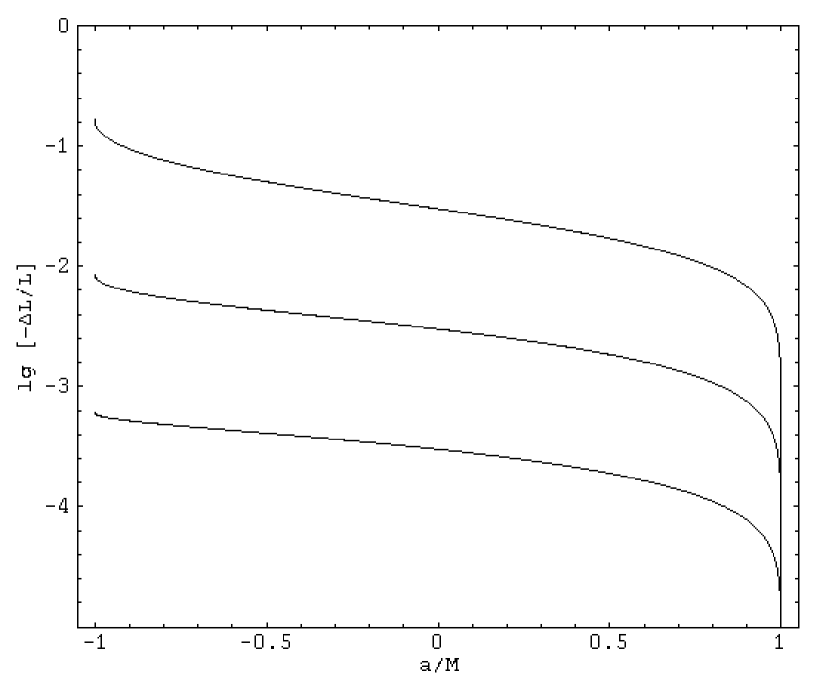
Figure 12: The change in the specific angular momentum of fluid particles as they approach the event horizon of the black hole [Eq. (104)], as a function of the spin of the black hole. It is assumed that the fast critical point is at $r\approx r_{\rm ms}$ . The magnetic field is parallel to the velocity field of the fluid, then the specific energy of fluid particles keeps constant in the plunging region, which we have assumed to be equal to the specific energy of a particle moving on the marginally stable circular orbit. The boundary value of the magnetic field at $r=r_{\rm ms}$ is specified by the ratio $\eta_{1}=B^{2}/4\pi\rho_{\rm m}$. The three curves corresponds to three different values of $\eta_{1}$ at $r=r_{\rm ms}$ : $10^{-2}$, $10^{-3}$, and $10^{-4}$ (downward).

and presented the results in Fig. 12.

To make the solutions smoothly joined to those in the disk region, in our calculations we have adopted that the specific energy is equal to that of a particle moving on the marginally stable circular orbit. Then, we have $f_{\rm E}=-E_{\rm ms}$. From Eqs. (100) and (101), on the marginally stable circular orbit there is a one-to-one correspondence between $c_{0}^{2}$ and

$$\eta_{1}=\frac{B^{2}}{4\pi\rho_{\rm m}}=\frac{c_{\rm A}^{2}}{1-c_{\rm A}^{2}}\;.$$ (105)

Therefore, we use $\eta_{1}$ at $r=r_{\rm ms}$ to specify the boundary value of the magnetic field, then $c_{0}$ is determined (up to a sign — which is not relevant here). Then, with the above approach, $f_{\rm L}$ is determined as a function of $\eta_{1}$ and $f_{\rm E}$. We have chosen $\eta_{1}$ to be $10^{-2}$, $10^{-3}$, and $10^{-4}$, alternatively.

From Fig. 12 we see that, though $L$ is not constant in the plunging region, its variation is extremely small, if on the marginally stable circular orbit the dynamical effects of the magnetic field on the motion of the fluid particles is negligible (then $\eta_{1}\ll 1$ at $r=r_{\rm ms}$). As $a/M$ increases from $-1$ to $1$, the variation in the specific angular momentum decreases, caused by the fact that the coordinate distance between the marginally stable circular orbit and the event horizon decreases with increasing $a/M$. For a black hole with $a/M\geq 0$, we have $|\Delta L/L|<3\%$ if $\eta_{1}<10^{-2}$ on $r=r_{\rm ms}$. For the extreme case of $a/M=1$, we have $|\Delta L/L|=0$, i.e. the specific angular momentum does not change at all. For the extreme case of $a/M=-1$, which has the largest coordinate distance from the marginally stable circular orbit to the event horizon, the variation in $L$ is largest. However, even in this case, the variation in the specific angular momentum is also not big: $|\Delta L/L|<17\%$ if $\eta_{1}<10^{-2}$ on $r=r_{\rm ms}$.

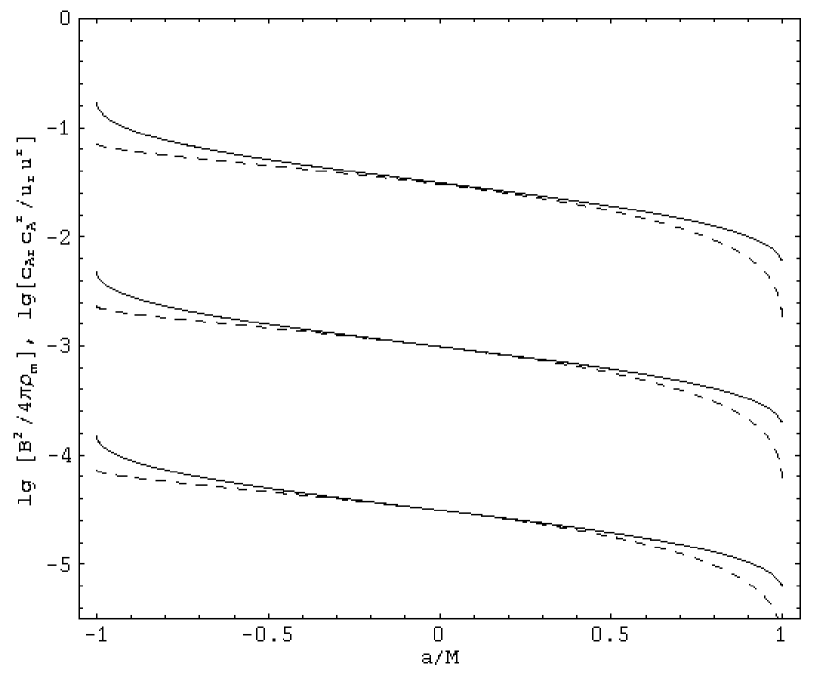
Figure 13: Same as Fig. 12 but for the ratios $B^{2}/4\pi\rho_{\rm m}$ (solid curves) and $c_{{\rm A}r}c_{\rm A}^{~{}\,r}/u_{r}u^{r}$ (dashed curves) at $r=r_{\rm H}$ .

For the same models we have also calculated the ratios $\eta_{1}$ and $c_{{\rm A}r}c_{\rm A}^{~{}~{}r}/u_{r}u^{r}$ at $r=r_{\rm H}$, and presented the results in Fig. 13. Because of Eq. (105), the value of $\eta_{1}$ is given by the left-hand side of Eq. (100). The ratio $c_{{\rm A}r}c_{\rm A}^{~{}~{}r}/u_{r}u^{r}$ can be calculated by

$$\frac{c_{{\rm A}r}c_{\rm A}^{~{}~{}r}}{u_{r}u^{r}}=\frac{c_{0}^{2}f_{\rm E}^{2}}{c_{0}^{2}\left(f_{\rm E}^{2}-1+\frac{2M}{r}\right)-r^{2}u^{r}}\;.$$ (106)

From Fig. 13 we see that both $B^{2}/4\pi\rho_{\rm m}$ (solid curves) and $c_{{\rm A}r}c_{\rm A}^{~{}~{}r}/u_{r}u^{r}$ (dashed curves) are small at $r=r_{\rm H}$. For $a/M\geq 0$, both are $<0.03$ if $\eta_{1}<10^{-2}$ at $r=r_{\rm ms}$. The ratios go down as $a/M$ increases. Even for the extreme case of $a/M=-1$, the ratios are also not big at $r=r_{\rm H}$ if $\eta_{1}<10^{-2}$ at $r=r_{\rm ms}$: $B^{2}/4\pi\rho_{\rm m}<0.18$ and $c_{{\rm A}r}c_{\rm A}^{~{}~{}r}/u_{r}u^{r}<0.07$.

Eq. (102) implies that $u_{\rm H}^{r}$ is always finite. Then, $u_{r}u^{r}=(r^{2}/\Delta)\left(u^{r}\right)^{2}\rightarrow\infty$ at $r=r_{\rm H}$ since $\Delta(r=r_{\rm H})=0$. Then, Eq. (106) implies that $c_{{\rm A}r}c_{\rm A}^{~{}~{}r}\rightarrow\infty$ also at $r=r_{\rm H}$ since its right-hand side is finite. However, from Eq. (99) we have

$$\left.\frac{c_{{\rm A}r}c_{\rm A}^{~{}\,r}}{u_{r}u^{r}}\right|_{r=r_{\rm H}}<1\;,$$ (107)

since $1-2M/r_{\rm H}=-a^{2}/r_{\rm H}^{2}$ and $u_{\rm H}^{r}<0$ .

Since $u_{\rm H}^{r}$ is finite, Eqs. (100) and (105) imply that $\eta_{1}$ is also finite at $r=r_{\rm H}$. Then, since $u_{r}u^{r}\rightarrow\infty$ at $r=r_{\rm H}$, we must have

$$\left.\frac{c_{\rm A}^{2}/(1-c_{\rm A}^{2})}{u_{r}u^{r}}\right|_{r=r_{\rm H}}=0\;.$$ (108)

Eqs. (107) and (108) imply that fluid particles always supersonically fall into the black hole. The numerical results in Fig. 13 confirm this conclusion.

From Figs. 10 – 13, we can demonstrate that when the boundary condition (84) [or, equivalently, (86)] is satisfied, the dynamical effects of magnetic fields in the plunging region are unimportant if they are so on the marginally stable circular orbit.

VII Summary and Discussion

With a simple model we have studied the evolution of magnetic fields in the plunging region around a Kerr black hole. The model contains the following assumptions: (1) The background spacetime is described by the Kerr metric; (2) The plasma is perfectly conducting so that the magnetic field is frozen to the plasma fluid; (3) The kinematic approximation bal98 applies, i.e. the dynamical effects of the magnetic field on the fluid motion are negligible so that the plasma fluid flows along timelike geodesics toward the central black hole; (4) In a small neighborhood of the equatorial plane (i.e., $|\pi/2-\theta|\ll 1$) the magnetic field and the velocity field have only radial and azimuthal components. The assumption (4) implies that $u^{\theta}=B^{\theta}=0$ and $\partial u^{\theta}/\partial\theta=\partial B^{\theta}/\partial\theta=0$ on the equatorial plane. With above assumptions, we have exactly solved Maxwell’s equations for axisymmetric solutions (i.e. $\partial/\partial\phi=0$). The solutions are given by Eqs. (50a) and (50b) [or, equivalently, Eqs. (52a) and (52b)], where $C_{0}$ is a constant measuring the magnetic flux through a circle in the equatorial plane, $\Psi$ is a function determining the time-evolution of the magnetic field. Both $C_{0}$ and $\Psi$ are determined by the boundary conditions.

The dependence of the solutions on the coordinate time $t$ is given by the function $\Psi=\Psi(t-\tau)$, where $\tau=\tau(r)$ is defined by Eq. (42). The function $\Psi$ is uniquely determined by the initial and boundary conditions of the magnetic field. The general form of $\Psi$ determines the retarded nature of the solutions: at any time the state of the magnetic field at a radius in the plunging region is determined by the state of the magnetic field at a larger radius and an earlier time (Figs. 1 and 2). This suggests that the stationary state of the magnetic field in the plunging region is uniquely determined by the boundary conditions at the marginally stable circular orbit.

Examples for the evolution of magnetic fields in the plunging region are shown in Figs. 3 – 8, for both the stationary case ($\Psi={\rm constant}$, Figs. 3 – 5) and the non-stationary case ($\Psi\neq{\rm constant}$, Figs. 6 – 8). From these figures we see that, the boundary value of the radial component of the magnetic field at the marginally stable circular orbit is more important in determining the strength of the magnetic field in the plunging region than the toroidal component. The initially toroidal component is attenuated in the plunging region by the radial expansion of the fluid (Fig. 3). The initially radial component is amplified by the azimuthal and vertical compression (the convergence of the fluid), and a toroidal component is generated from the radial component by the shear motion of the fluid though the toroidal component is initially zero at the marginally stable circular orbit (Fig. 4). This leads to the amplification of the magnetic field in the plunging region (Fig. 5). The evolution of the magnetic field depends on the spinning state of the black hole, but is more sensitive to the initial value of the radial velocity on the marginally stable circular orbit [or, equivalently the parameter $\delta$ defined by Eq. (59)].

The time-evolution of magnetic fields shown in Figs. 6 – 8 confirms our claim that the stationary state of the magnetic field in the plunging region is uniquely determined by the boundary conditions on the marginally stable circular orbit. If in the plunging region a magnetic field is initially deviated from the stationary solutions, it will evolve to and finally get saturated at the state given by the stationary solutions in a dynamical time scale determined by the free-fall motion of fluid particles in the plunging region. If the magnetic field on the marginally stable circular orbit is in a stationary state, the magnetic field in the plunging region will automatically settle into a stationary state. Thus, the evolution of magnetic fields in the plunging region is very different from that in the disk region, in the latter case the state of the magnetic field is determined by the local MHD processes. The difference is caused by the following fact: in the disk region the fluid has a very small radial velocity so that local MHD processes have shorter time scales than the radial motion; in the plunging region the fluid has a large radial velocity so that local MHD processes usually have longer time scales than the radial motion.

In deriving the solutions we have assumed that the dynamical effects of the magnetic field in the plunging region are unimportant [the kinematic approximation adopted in assumption (3)]. To justify this assumption, we have studied the dynamical effects of magnetic fields in the stationary state in two ways. First, we estimate the dynamical effects of magnetic fields by considering the back-reaction: substituting the solutions of Maxwell’s equations we obtained, where we assumed that fluid particles move on geodesics, into the dynamical equations to check if the motion of the fluid is significantly affected by magnetic fields. In this way, we estimate the dynamical effects of magnetic fields on the motion of the fluid by calculating the parameters $\eta_{1}$, $\eta_{2}$ and $\eta_{3}$ defined by Eq. (80). The mass density of the fluid, which appears in the denominators of $\eta_{1}$, $\eta_{2}$ and $\eta_{3}$, drops quickly in the plunging region if $|v_{\hat{r}}|\ll|v_{\hat{\phi}}|$ on the marginally stable circular orbit (Fig. 9). However, the evolution of the magnetic field, which appears in the numerators of $\eta_{1}$, $\eta_{2}$ and $\eta_{3}$, sensitively depends on the orientation of the magnetic field on the marginally stable circular orbit, the latter is essentially determined by the MHD processes in the disk region. If we require that the solutions in the plunging region are smoothly joined to the solutions in the thin Keplerian disk region, then it is reasonable to assume that on the marginally stable circular orbit, as well as in the disk region, the magnetic field is parallel to the velocity field: $B^{r}/B^{\phi}=u^{r}/u^{\phi}$ (see the Appendix). This implies that for the solutions in the plunging region we should have $\Psi=0$ [Eq. (86)], i.e. the orientation of the magnetic field follows the orientation of the velocity field of the fluid [Eq. (84)]. With such a boundary condition, we have calculated $\eta_{1}$, $\eta_{2}$ and $\eta_{3}$ , assuming that particles move on geodesics. We see that, if they are $\ll 1$ on the marginally stable circular orbit, then they remain so in the plunging region (Figs. 10 and 11). Indeed, $\eta_{1}$, $\eta_{2}$ and $\eta_{3}$ decrease in the plunging region for sufficiently small $|v_{\hat{r}}|$ on the marginally stable circular orbit.

Second, we self-consistently solve the coupled Maxwell and dynamical equations on the horizon of the black hole, check how much has changed in the specific angular momentum of fluid particles since they leave the marginally stable circular orbit. The specific energy of fluid particles is not changed by a magnetic field that satisfies $\Psi=0$ [see Eq. (92)]. However, the specific angular momentum does change [see Eq. (91)]. We have calculated the specific angular momentum of fluid particles as they reach the horizon of the black hole, assuming that the fluid particles pass the fast critical point near the marginally stable circular orbit. The deviation from the specific angular momentum as the particles just leave the marginally stable circular orbit is shown in Fig. 12. We see that, though the specific angular momentum of fluid particles is changed by the magnetic field, the effects are always small assuming that on the marginally stable circular orbit the dynamical effects of the magnetic field are not important. For example, for $a/M\geq 0$ we have $|\Delta L/L|<3\%$ if $\eta_{1}<10^{-2}$ on the marginally stable circular orbit. We have also calculated the ratios $\eta_{1}=B^{2}/4\pi\rho_{\rm m}$ and $c_{{\rm A}r}c_{\rm A}^{~{}\,r}/u_{r}u^{r}$ on the horizon (Fig. 13), where $c_{\rm A}^{~{}\,r}$ is the radial component of the Alfvén velocity. These two ratios are relevant to the critical points in the flow [see Eqs. (99), (100), and (105)] and measure at what level the magnetic field affects the motion of the fluid. Fig. 13 shows that their values on the horizon are quite small.

Both approaches (back-reaction and self-consistent solutions) confirm that the dynamical effects of the magnetic field are unimportant in the plunging region if they are so on the marginally stable circular orbit.

Our results differ from that of Gammie gam99 , in which he claimed that in the plunging region the dynamical effects of magnetic fields can be important. The difference is caused by the fact that Gammie used a boundary condition that is different from ours for the magnetic field. Gammie assumed that $\Psi=-\Omega_{\rm ms}C_{0}$, where $\Omega_{\rm ms}$ is the angular velocity of the disk at the marginally stable circular orbit, while we assume that $\Psi=0$. Gammie’s boundary condition implies that $v_{\hat{r}}=0$ at $r=r_{\rm ms}$ (as clearly stated in his paper), which makes $r=r_{\rm ms}$ a singular point where $\rho_{\rm m}=\infty$ (to keep the mass flux $F_{\rm m}$ nonzero). Hence, Gammie’s solutions are not well-behaved at the marginally stable circular orbit. Our boundary condition allows the solutions in the plunging region to be smoothly joined to the solutions in the disk region (see the Appendix), since in our solutions all physical quantities are finite at the marginally stable orbit. Certainly, to precisely take care of the transition from the disk region to the plunging region, gas pressure and non-electromagnetic stress must be properly taken into account near the inner edge of the disk.

As mentioned in the Introduction, recently the “no-torque inner boundary condition” for thin accretion disks has been challenged by some authors (including Gammie) based on their studies on the evolution of magnetic fields in the plunging region kro99 ; gam99 ; haw01b ; haw02 . The results in this paper suggest that in the plunging region the dynamical effects of the magnetic field are not important, if the solutions in the plunging region are smoothly joined to the the solutions in the thin Keplerian disk region. Thus, the argument against the “no-torque inner boundary condition” is not founded.

Finally, we note that in the paper we have neglected dissipative processes like magnetic reconnection and ohmic dissipation, and the evaporation effect arising from the magnetic buoyancy and MHD instabilities. These processes operate in disks to limit the amplification of magnetic fields (gal79, ; tou92, ; bal98, , and references therein). Certainly it is conceivable that they can also operate in the plunging region to reduce the amplification effect of magnetic fields. If these processes are important, the results of this paper tend to overestimate the amplification of magnetic fields in the plunging region. Then, the dynamical effects of magnetic fields should be weaker than that we have estimated without considering dissipative processes, which will strengthen our conclusion that the dynamical effects of magnetic fields are unimportant in the plunging region.

Appendix A Magnetic Fields in the Disk Region

In the disk region ($r>r_{\rm ms}$), viscosity plays an important role in the dynamics of disk particles. The viscosity transports angular momentum outward and dissipates energy, which leads to disk accretion. So, in the disk region, particles move on non-geodesic worldlines.

In the vertical direction, the gravity of the black hole is balanced by the gradient of the total pressure (= gas pressure + radiation pressure + magnetic field pressure) in the disk. Therefore, in a small neighborhood of the disk central plane, disk particles are more likely moving on planes parallel to the equatorial plane, rather than moving radially as in the plunging region. To describe such a motion, cylindrical coordinates $(t,r,\phi,z)$ are more suitable, where $t$ and $\phi$ have the same meaning as those in the Boyer-Lindquist coordinates, to the first order $r$ also has the same meaning as that in the Boyer-Lindquist coordinates, but $z\equiv r\left(\frac{\pi}{2}-\theta\right)$ where $\left|\frac{\pi}{2}-\theta\right|\ll 1$ .

In the cylindrical coordinates, in a small neighborhood of the disk central plane the Kerr metric can be written as pag74

$$ds^{2}=-\left(1-\frac{2M}{r}\right)dt^{2}-\frac{4Ma}{r}\,dtd\phi+\frac{r^{2}}{\Delta}\,dr^{2}+\frac{A}{r^{2}}\,d\phi^{2}+dz^{2}\;,$$ (109)

where $\Delta$ and $A$ are defined by Eq. (17) with $\theta=\pi/2$ .

The Maxwell equations that we need to solve are again given by Eq. (31), but now we have $x^{\alpha}=(t,r,\phi,z)$ and $\sqrt{-g}=r$. As in the case for the plunging region, we assume that the motion of fluid particles is stationary but the evolution of the magnetic field can depend on time, i.e., we let $\partial u^{\alpha}/\partial t=0$ but keep $\partial B^{\alpha}/\partial t$ in the Maxwell equations. Furthermore, we assume that in a small neighborhood of the disk central plane $u^{z}=B^{z}=0$ so that $\partial u^{z}/\partial z=\partial B^{z}/\partial z=0$ on the equatorial plane. Finally, we adopt $\partial u^{\alpha}/\partial\phi=\partial B^{\alpha}/\partial\phi=0$ because of the axisymmetry of the system. Then, on the equatorial plane Eq. (31) is reduced to

$$\frac{\partial}{\partial t}\left[r(u^{t}B^{\beta}-u^{\beta}B^{t})\right]+\frac{\partial}{\partial r}\left[r(u^{r}B^{\beta}-u^{\beta}B^{r})\right]=0\;.$$ (110)

Eq. (110) can be solved with the same approach as that used in Sec. IV. The solutions are

$$B^{r} = \frac{1}{r}(-C_{0,{\rm d}}u_{t}+\Psi_{\rm d}u_{\phi})\;,$$ (111a)

$$B^{\phi} = \frac{1}{ru^{r}}[-C_{0,{\rm d}}u_{t}u^{\phi}+(1+u^{\phi}u_{\phi})\Psi_{\rm d}]\;,$$ (111b)

where $C_{0,{\rm d}}$ is an integral constant, $\Psi_{\rm d}=\Psi_{\rm d}(t-\tau)$ is the solution of Eq. (40). The corresponding $B^{t}$ is related to $B^{r}$ and $B^{\phi}$ by Eq. (38).

Eq. (111a) can be written as

$$\Psi_{\rm d}=\frac{1}{u_{\phi}}(rB^{r}+C_{0,{\rm d}}u_{t})\;.$$ (112)

Assume that as $r\rightarrow\infty$ the disk is Keplerian so that $u_{\phi}=L\propto r^{1/2}$ and $u_{t}=-E\approx 1$, and $rB^{r}$ keeps finite, then we must have

$$\lim_{r\rightarrow\infty}\Psi_{\rm d}=0\;.$$ (113)

Eq. (113) has an important implication for stationary solutions. For stationary solutions we have $\Psi_{\rm d}={\rm constant}$, then by Eq. (113) we must have $\Psi_{\rm d}=0$. So, for stationary solutions we have

$$B^{r} = \frac{C_{0,{\rm d}}E}{r}\;,$$ (114a)

$$B^{\phi} = \frac{C_{0,{\rm d}}Eu^{\phi}}{ru^{r}}\;,$$ (114b)

where we have used $u_{t}=-E$.

From Eqs. (114a) and (114b) we have $B^{\phi}/B^{r}=u^{\phi}/u^{r}$, i.e. in the stationary state the magnetic field lines are parallel to the fluid motion.

References

- (1) J. Frank, A. King, and D. J. Raine, Accretion Power in Astrophysics (Cambridge University Press, Cambridge, England, 2002).
- (2) S. Kato, J. Fukue, and S. Mineshige, Black-Hole Accretion Disks (Kyoto University Press, Kyoto, Japan, 1998).
- (3) I. D. Novikov and K. S. Thorne, in Black Holes, edited by C. DeWitt and B. S. DeWitt (Gordon and Breach, New York, 1973), P. 343.
- (4) D. N. Page and K. S. Thorne, Astrophys. J. 191, 499 (1974).
- (5) B. Muchotrzeb and B. Paczyński, Acta Astr. 32, 1 (1982).
- (6) M. A. Abramowicz and S. Kato, Astrophys. J. 336, 304 (1989).
- (7) B. Paczyński, preprint astro-ph/0004129 (2000).
- (8) P. J., Armitage, C. S. Reynolds, and J. Chiang, Astrophys. J. 548, 868 (2001).
- (9) N. Afshordi and B. Paczyński, preprint astro-ph/0202409 (2002).
- (10) S. A. Balbus and J. F. Hawley, Rev. Mod. Phys. 70, 1 (1998).
- (11) J. K. Krolik, Astrophys. J. Lett. 515, L73 (1999).
- (12) C. F. Gammie, Astrophys. J. Lett. 522, L57 (1999).
- (13) E. Agol and J. H. Krolik, Astrophys. J. 528, 161 (2000).
- (14) J. F. Hawley, Astrophys. J. 528, 462 (2000).
- (15) J. F. Hawley, Astrophys. J. 554, 534 (2001).
- (16) J. F. Hawley and J. H. Krolik, Astrophys. J. 548, 348 (2001).
- (17) J. F. Hawley and J. H. Krolik, Astrophys. J. 566, 164 (2002).
- (18) R. D. Blandford, in Accretion Processes in Astrophysical Systems: Some Like It Hot! edited by S. S. Holt and T. R. Kallman (AIP, New York, 1998), P. 43.
- (19) L. -X. Li, Astrophys. J. Lett. 533, L115 (2000).
- (20) L. -X. Li and B. Paczyński, Astrophys. J. Lett. 534, L197 (2000).
- (21) L. -X. Li, Astrophys. J. 567, 463 (2002).
- (22) L. -X. Li, Phys. Rev. D 65, 084047 (2002).
- (23) J. Wilms et al., Mon. Not. Roy. Ast. Soc 328, L27 (2001).
- (24) L. -X. Li, Astron. Astrophys. 392, 469 (2002).
- (25) J. M. Miller et al., Astrophys. J. 570, L69 (2002).
- (26) C. W. Misner, K. S., Thorne, and J. A. Wheeler, Gravitation (W. H. Freeman, San Francisco, 1973).
- (27) R. M. Wald, General Relativity (The University of Chicago Press, Chicago, 1984).
- (28) A. Lichnerowicz, Relativistic Hydrodynamics and Magnetohydrodynamics (W. A. Benjamin, INC., New York, 1967).
- (29) S. W. Hawking and G. F. R. Ellis, The Large Scale Structure of Space-Time (Cambridge University Press, London, England, 1973).
- (30) R. K. Sachs and H. Wu, General Relativity for Mathematicians (Springer-Verlag, New York, 1977).
- (31) J. M. Bardeen, W. H. Press, and S. A. Teukolsky, Astrophys. J. 178, 347 (1972).
- (32) K. S. Thorne, R. H. Price, and D. A. Macdonald, Black Holes: The Membrane Paradigm (Yale University Press, New Haven, 1986).
- (33) E. J. Weber and L. Davis, Astrophys. J. 148, 217 (1967).
- (34) H. J. G. L. M. Lamers and J. P. Cassinelli, Introduction to Stellar Winds (Cambridge University Press, Cambridge, England, 1999).
- (35) A. A. Galeev, R. Rosner, and G. S. Vaiana, Astrophys. J. 229, 318 (1979).
- (36) C. A. Tout and J. E. Pringle, Mon. Not. R. Astron. Soc., 259, 604 (1992).