A simplified numerical model of coronal energy dissipation based on reduced MHD

A 3D model intermediate between cellular automata (CA) models and the reduced magnetohydrodynamic (RMHD) equations is presented to simulate solar impulsive events generated along a coronal magnetic loop. The model consists of a set of planes distributed along a magnetic loop between which the information propagates through Alfvén waves. Statistical properties in terms of power-laws for energies and durations of dissipative events are obtained, and their agreement with X-ray and UV flares observations is discussed. The existence of observational biases is also discussed.

1 Introduction

One of the main unresolved problems in solar physics concerns the mechanism by which the solar atmosphere is heated from several thousands degrees in the photosphere to millions in the corona. It is now commonly accepted that the ultimate source of energy lies in the convective motions in and below the photosphere, and that a reliable model of coronal heating has to deal with the transfer, the storage and finally the release of this energy into the solar corona. Several conceptual models have been proposed, such as Alfvén waves, electric currents and MHD turbulence – see for a review Zirker (1993) – where in all cases the magnetic field plays a key role in the dynamics.

On the other hand, it is also well established that impulsive events (e.g. solar flares, X-ray bright points) are distributed in the corona over a large range of scales in size, energy and duration (Dennis, 1985; Crosby, Aschwanden & Dennis, 1993; Pearce, Rowe & Yeung, 1993; Krucker & Benz, 1998; Aletti et al., 2000; Aschwanden et al., 2000) and that large events seem to be made up of the superposition of a myriad of smaller unresolved events. It was Parker (1988) who suggested that the active X-ray and UV corona is composed of a swarm of localized impulsive bursts of energy called nanoflares (or picoflares). Much theoretical work has been done to investigate Parker’s conjecture and more generally the statistical nature of the solar coronal heating. They mainly follow two complementary schools which refer on the one hand to the dynamics of complex systems and on the other hand to fluid mechanics.

The statistical properties of flaring activity allow one to view the solar corona as a complex system which can be described with cellular automata (CA) models (Lu & Hamilton, 1991; Lu et al., 1993; Vlahos et al., 1995; Galsgaard, 1996; Georgoulis & Vlahos, 1998; Vassiliadis et al., 1998; Isliker, Anastasiadis & Vlahos, 2000, 2001; Charbonneau et al., 2001; Krasnoselskikh et al., 2001). CA models have become increasingly useful in the study of complex systems because they permit the study of an entire system without ignoring the effects of individual components of the system. There are many natural applications such as substorms in the magnetotail (Takalo et al., 1999), star formation in spiral galaxies (Lejeune & Perdang, 1996) or earthquakes (Carlson & Langer, 1989). A cellular automaton is based upon the idea of the locality of influence : a system is distributed in space, and nearby regions have more influence than those far apart (see for instance MacKinnon & Macpherson (1997) for a study of a nonlocal communication). A grid of cells is used to represent the components of a system, and each cell is given a set of phenomenological rules concerning its surrounding neighbors. The system evolves over several iterations by allowing each cell to interact using the given rules. What makes CA so interesting and useful is that after many iterations they reveal complex structures and arrangements that form across great distances even though each cell only takes into account local information. Self-Organized Criticality (SOC) (Bak et al., 1987; Kadanoff et al., 1989; Hwa & Kardar, 1992; Sornette, 2000) refers to the spontaneous organization of such an externally driven system into a globally stationary state over many scales.

On the other hand, we find fluid models which give the physical description that is missing in CA. Much work has been done on statistical solar flares (Longcope & Sudan, 1994; Walsh, Bell & Hood, 1995; Einaudi et al., 1996; Galsgaard & Nordlund, 1996; Hendrix & Van Hoven, 1996; Dmitruk et al., 1998; Galtier & Pouquet, 1998; Georgoulis et al., 1998; Galtier, 1999; Walsh & Galtier, 2000) but most of them suffer from the fact that statistical simulations of flares studied in the context of forced resistive MHD equations are possible only at the cost of huge computational expenses. Nevertheless it has been possible to show important properties, e.g. that the dissipative events produced exhibit power-law distributions (for total energy, peak of luminosity and duration) in agreement with X-ray observations, but with generally a much smaller “inertial range” than the CA counterpart.

A recent debate about the possible existence of sympathetic flaring, i.e. the correlation in time of two successive events (Pearce, Rowe & Yeung, 1993; Wheatland, Sturrock & McTiernan, 1998; Boffetta et al., 1999; Wheatland, 2000; Lepreti, Carbone & Veltri, 2001; Galtier, 2001), suggests the possibility to dismiss CA as a model of solar flares since standard CA models do not produce correlated events (non-Poissonian statistics such as power-law waiting time distributions). But in fact many CA models exist in the literature like nonconservative models (Christensen & Olami, 1992) which turn out to be able to generate the statistics expected for sympathetic flaring. But the question of the existence of sympathetic flaring in the corona has not yet found an answer since in particular there is still a debate about what we mean by event.

The problem of coronal heating is intimately linked to the existence of nanoflares whose Probability Distribution Function (PDF) in energy is supposed to be a power-law steeper than that for regular flares. Let us assume that the PDF in energy $E$ of events is distributed according to a power-law of index $-\zeta$, i.e. $\Pr(E)\propto E^{-\zeta}$. It is then possible to show that there exists a critical slope of index $\zeta_{c}=2$ (Hudson, 1991). Indeed, the total energy released in the corona by events between $E_{min}$ and $E_{max}$ is $(E_{max}^{2-\zeta}-E_{min}^{2-\zeta})/(2-\zeta)$ which means that if $\zeta<2$ the main contribution comes from high energy events, whereas if $\zeta>2$ it comes from smaller events (the swarm of nanoflares). The average power dissipated in a large flare is of the same order of magnitude as the total average power emitted by the corona, $\simeq 10^{3}\>\mathrm{W}\cdot\>\mathrm{m}^{-2}$, which proves that regular flares can not account for coronal heating since they are episodic events seen over and above the average coronal background. It is then natural to think that a swarm of very small and still unobservable events may dominate the heating process. One of the main challenges of statistical flare models is to know whether or not it is possible to produce power-law distributions for any relevant quantity such as energy, luminosity or duration, and what the power-law indices are.

The aim of this paper is to introduce a hybrid model for a solar magnetic loop which is somewhat intermediate between CA models and full MHD or reduced MHD models. In this model, we will inject and store energy into a coronal loop (our numerical domain) via wave propagation from the photosphere (our numerical boundary). The trigger for an event is determined in a way analogous to conventional CA models, i.e. with a threshold in the current. However, during the subsequent event the current is dissipated and the magnetic field recomputed using Maxwell’s equations. Let us note that this is a minimal consistency requirement for the field evolution which is not always incorporated in CA models. In practice, the model allows current concentrations to form kinematically (advection from the photosphere), but not dynamically (the nonlinear part of the Lorenz force, $\@vec{j}\times\@vec{b}$). The model is non-trivial because of the threshold dynamics of the dissipation, which mimics the nonlinear terms, but the model is much simpler to integrate than the full MHD equations, therefore allowing a fast computation of statistics (events sizes and durations), and a comparison both with observations and full numerical simulations.

The paper is organized as follows. In Section 2 we give a detailed description of the CA model and show its basic behavior through some numerical experiments. In Section 3 the results of a parametric study are given and discussed. In Section 4 we summarize the properties of the model, we present a comparison with observations, and we draw some conclusions.

2 The model

In the original 3D lattice model developed by Lu & Hamilton (1991) the physical quantity defined on each lattice is the magnetic field. The system is driven from the outside by adding randomly in space a random magnetic field. The process continues until a reconnection instability criterion is satisfied at any point of the 3D lattice, i.e. until the magnetic gradient exceeds a critical value at this point. Then the magnetic field is redistributed (diffused) towards neighboring nodes with the possibility to transfer the instability as well. The redistribution process stops when the system is completely relaxed. Then another random amount of magnetic field is added to the system. An event called avalanche is associated to the rapid diffusion of the magnetic field.

Subsequent models use the magnetic vector potential $\@vec{A}$ rather than the magnetic field since the divergence-free condition for the magnetic field is then automatically satisfied. For example in the recent model developed by Isliker, Anastasiadis & Vlahos (2000, 2001) where the 3D lattice represents an ensemble of magnetic loops, the knowledge of $\@vec{A}$ allows to reconstruct the magnetic field topology and eventually the structure of the current density. To do so they introduce the notion of derivative. The present simplified model belongs to this class of models but only one typical coronal loop will be considered and simulated. The detailed description of the model is now given.

2.1 Basic idea : on-off mechanism and turbulence

A possible reason for the behavior of the corona is that it lies in a turbulent state. A model of coronal loops should therefore allow for the effects of turbulent fluctuations. This is possible with CA models at a very superficial level through an on-off mechanism. The idea behind the threshold dynamics of our model, the on-off mechanism, is the following. The forcing due to the convective granules, although applied on a range of scales, has a typical length scale that is supposed to be far greater than the dissipative scale. The connection between the forcing and the dissipative length scales is made through a turbulent mechanism. During the “off” phase, i.e. the loading phase, the plasma is in a laminar state where the dynamics is essentially governed by the linear terms (and the loading). Because the system is driven slowly, parts of the system or even the entire system can stay in principle in this state for very long periods of time. When sufficient energy is accumulated in the loop some nonlinear instability appears which triggers the rapid generation of small scales. The inertial range of the turbulent energy spectrum extends to small scales and makes the link between the typical forcing length scale and the dissipative length scale. This “on” phase is therefore characterized by a sudden increase of the dissipative terms in the RMHD equations (see section 2.2) leading to a bursty event. Then the system returns immediately to an “off” phase. The nonlinearities of the RMHD equations are therefore included in the model in a very schematic way through a threshold dynamics only.

2.2 Description of the model

Geometry of the model.

The model describes a coronal loop anchored in the photosphere whose footpoints are randomly moved. The presence of a strong axial magnetic field leads to essentially 2D dynamics, i.e. perpendicular to the mean magnetic field, for which the approximation of the RMHD equations (Strauss, 1976) is a good model. As we can see on Fig. 1, the 3D regular grid is made up of a set of planes distributed along the loop between which the information propagates through Alfvén waves. Therefore each plane will evolve essentially independently from each other. Both boundary planes represent the photospheric footpoints, while the intermediate planes represent the loop itself, as if it were unbent. The curvature of the loop is not taken into account since the width of observed coronal loops (see e.g. observations from the TRACE instrument) appears to be constant along the loop and is much smaller than their length.

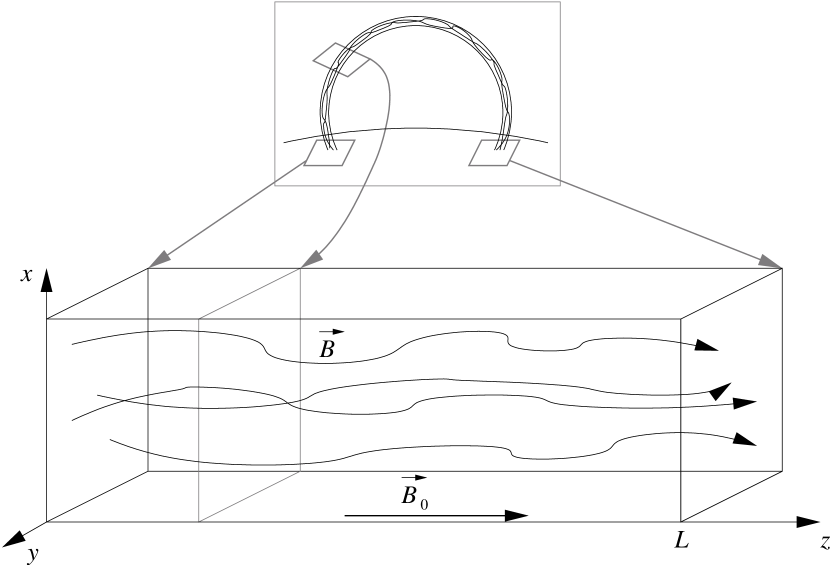
Figure 1: Model of coronal loop used for the simulations : the loop is unbent into a box, whose both extreme planes represent the photosphere. Parallel planes represent slices orthogonal to the local direction of the loop.

RMHD equations.

Our aim is to compute the temporal evolution of the velocity field $\@vec{v}$ and the magnetic field $\@vec{B}$ (or $\@vec{b}\equiv\@vec{B}/\sqrt{\rho_{0}\mu_{0}}$ if we consider only fields with the same physical dimension). We assume the presence of a strong and uniform axial magnetic field along the $z$-axis $\@vec{b}_{0}=b_{0}\@vec{e}_{z}$ ($\equiv\@vec{B}_{0}/\sqrt{\rho_{0}\mu_{0}}$) and we consider small perturbations to this field. We separate $\@vec{b}-\@vec{b}_{0}$ and $\@vec{v}$ into parallel components ($b_{z}\@vec{e}_{z}$ and $v_{z}\@vec{e}_{z}$) and orthogonal components ($\@vec{b}_{\perp}$ and $\@vec{v}_{\perp}$). With the following additional hypotheses, (i) the scales along the $z$-axis are larger than the scales in the orthogonal directions (gradients along the $z$ axis are negligible), and (ii) the kinetic pressure is negligible compared to the magnetic pressure (i.e. the plasma is cold, $\beta\ll 1$), we then obtain the RMHD equations (Strauss, 1976)

$$\partial_{t}\@vec{v}_{\perp}+(\@vec{v}_{\perp}\cdot\@vec{\nabla}_{\perp})\@vec{v}_{\perp} = b_{0}\partial_{z}\@vec{b}_{\perp}+\nu\,\Delta_{\perp}\@vec{v}_{\perp}$$

$$+(\@vec{b}_{\perp}\cdot\@vec{\nabla}_{\perp})\@vec{b}_{\perp}-\@vec{\nabla}(b_{\perp}^{2}/2)\,,$$

$$\partial_{t}\@vec{b}_{\perp}+(\@vec{v}_{\perp}\cdot\@vec{\nabla}_{\perp})\@vec{b}_{\perp} = b_{0}\partial_{z}\@vec{v}_{\perp}+\eta\,\Delta_{\perp}\@vec{b}_{\perp}$$

$$+(\@vec{b}_{\perp}\cdot\@vec{\nabla}_{\perp})\@vec{v}_{\perp}\,,$$

where $\nu$ and $\eta$ are respectively the kinematic viscosity and the magnetic resistivity. To each grid point are associated two scalar fields $a^{s}$, with $s=\pm$, from which the Elsässer fields are derived

$$\@vec{z}^{s}=\@vec{v}_{\perp}+s\@vec{b}_{\perp}=\@vec{\nabla}_{\perp}\times a^{s}\@vec{e}_{z}\,.$$ (3)

All other fields (magnetic and velocity fields, current density, vorticity…) are derived from $a^{s}$ by analogy with the standard magnetic and kinematic equations.

Initial state and boundaries.

The fields $a^{s}$ are taken to be zero initially. Each cross-sectional plane along the loop is periodic for the $a^{s}$ variables. All numerical computations for each plane are made in the Fourier space. We use inverse Fast Fourier Transforms (FFT) when we temporarily need to know the values of a field at some positions in real space.

Alfvén wave propagation.

In the right hand side of equations (2.2-2.2), the first terms correspond to the Alfvén waves propagation along the $z$-axis : $a^{+}$ propagates to the bottom of the simulation box (low values of $z$), while $a^{-}$ propagates to the top. These propagations are modeled by specific cellular automaton rules used at each time step $\delta t$ of the simulation, corresponding to discretization of the Alfvén waves terms of equations (2.2-2.2) in the form :

$$a^{s}(z,t+\delta t)=a^{s}(z+s\,\delta z,t)$$ (4)

There is no loss of energy (or reflection) during the Alfvén wave propagation since the density is assumed to be constant ; however we assume that there is a total reflection of the waves when they reach the photosphere, i.e. the two boundary planes of the simulation box.

Loading.

The action of the photospheric granules on the magnetic footpoints is modeled by a random increment $\delta\Psi$ to the fields on both boundary planes. This increment has random Fourier coefficients but has globally a power-law energy spectrum in $\sim k^{-\alpha}$ (the total intensity $P_{\mathrm{load}}=\int(k\,\delta\Psi)^{2}\,\mathrm{d}\@vec{k}$ is also a parameter of the simulation). Indeed, observational evidence suggests that the convective layer is in a turbulent state : the photospheric granules exhibit a turbulent power spectrum of velocity consistent with a Kolmogorov energy spectrum in $k^{-5/3}$ but only for a narrow inertial range of wavenumbers ($\ell\sim 1/k<3\>\mathrm{arcsec}$) (Roudier & Muller, 1986; Chou et al., 1991; Espagnet et al., 1993). We emphasize that there is no loading in the other parts of the loop : energy is solely carried by Alfvén waves. Furthermore, these waves reflect on both photospheric boundary planes.

Dissipation criterion.

We assume that dissipation occurs when an instability criterion is satisfied, which is the condition that the magnitude of the current density $\|\@vec{J}\|$ exceeds a critical value $J_{c}$. As $J_{z}=\@vec{J}\cdot\@vec{e}_{z}$ can be derived from the computed variables $a^{s}$ ($J_{x}$ and $J_{y}$ are negligible), this dissipation criterion is likely to have more physical meaning than the criteria used for example in classical sandpile and in more elaborate models (see Charbonneau et al. (2001) for a review). However, there is still some doubt about the quality of this criterion, as will be discussed later (see section 4.1).

Reconfiguration of the field.

When the current density exceeds a given threshold at some real-space grid points in a given plane, the nonlinear terms of equations (2.2-2.2) which are negligible during the loading phase (the off phase) become large and dominate the dynamics of the fields. They are quickly balanced by the dissipative terms when the energy cascade reaches the dissipative scale. This “on” phase (see section 2.1) is modeled by a diffusion-like process for the magnetic and velocity fields which tends to reduce the magnitude of the current density and the vorticity.

The detailed algorithm is an updated version of the one introduced by Einaudi & Velli (1999). At a time $t$ for plane $z_{0}$ we compute the current density $J_{z}(x,y,z_{0})=-\Delta_{\perp}A_{z}$, where $A_{z}=(a^{+}-a^{-})/2$ is the magnetic vector potential and $\Delta_{\perp}$ denotes the Laplacian operator in the plane $z_{0}$. If at some grid point $(x,y,z_{0})$ the value of $|J_{z}|$ exceeds the threshold $J_{c}$, $A_{z}$ is updated in the time $\delta t_{c}$ (with $\delta t_{c}\ll\delta t$ ) according to the equation $A_{z}(x,y,z_{0};t+\delta t_{c})=A_{z}(x,y,z_{0};t)-\eta\,\delta t_{c}\,J_{z}(x,y,z_{0};t)$, which corresponds to current dissipation. The current density $J_{z}$ corresponding to $A_{z}(t+\delta t_{c})$ is then computed, and this dissipation process is iterated until $J_{z}$ does not exceed the threshold anywhere in the plane $z_{0}$. However, note that after the first iteration of this process, we take $C\,J_{c}$ as a threshold instead of $J_{c}$. The “dissipation efficiency” $C$ is a number between $0$ and $1$ which guarantees that the system is in a relaxed state after the whole dissipation process.

Energy release

During this relaxation process, magnetic and kinetic energies are released. The energy release in each plane can easily be computed from the variations of $\langle\@vec{b}_{\perp}^{2}\rangle$ and $\langle\@vec{v}_{\perp}^{2}\rangle$ in the plane. It is the primary variable for our statistics. Note that topological modifications of the magnetic field may be expected : the connectivity of the magnetic field lines is modified because of the field diffusion. One of the possible interpretations of this phenomenon is magnetic reconnection (see however the discussion in section 4.1).

2.3 Time and space scales.

Let $\delta x$ and $\delta z$ be the distance between grid points in the $x$ (or $y$) and $z$ directions respectively, and let $\delta t$ be the time step. If we assume that the loop length $L$ is $1$ to $100\>\mathrm{Mm}$, then $\delta z$ is $30\>\mathrm{km}$ to $3\>\mathrm{Mm}$ for a typical resolution of $N_{L}=30$ points (i.e. 30 planes along $z$). The analog assumptions for a loop width $\ell$ ($=L/10$) of $0.1$ to $10\>\mathrm{Mm}$ give $\delta x$ between $1.5$ and $150\>\mathrm{km}$ for a typical resolution of $N_{\ell}=64$.

We can also determine time scales for the model : as the Alfvén speed is one in the model units, i.e. in units of $\delta z/\delta t$, we have $\delta t=\delta z/v_{A}$ : the time step is the time needed by the Alfvén wave to propagate from one plane to its neighbors. For $B_{0}=10^{-3}$ to $10^{-2}\>\mathrm{T}$ (i.e. $v_{A}\approx 1$ to $10\>\mathrm{Mm\,s^{-1}}$ with density $\rho_{0}\approx 10^{-12}\>\mathrm{kg\,m}^{-3}$), this yields $\delta t$ between $3\times 10^{-3}\>\mathrm{s}$ and $3\>\mathrm{s}$. Another time scale in the system is the coherence time of photospheric loading $\delta t_{l}$. It is modeled by a periodic re-initialization of the coefficients of the loading increment $d\Psi$, which occurs every $200$ time steps $\delta t$, or $0.6$ to $600\>\mathrm{s}$. This is small compared to observational evaluations of the photospheric coherence time, but the relevant point is the good separation between time scales ; besides, larger values of the photospheric loading coherence time do not alter the results of the model. When no other indication is given, the time step $\delta t$ is the unit of time ; for example, on Fig. 2, the $x$-axis range maximum is $10\,000\,\delta t$, i.e. between approximately $30\>\mathrm{s}$ and $8\>\mathrm{h}$. At last, the shortest time scale in the model is the cascade time scale $\delta t_{c}$, which is the time step for dissipations within a cascade, and which is analogous to the non-linear time scale of MHD models. It is assumed to be completely separated from the other time scales, i.e. $\delta t_{c}\ll\delta t\ll\delta t_{l}$.

A direct consequence of the separation between the cascade time scale $\delta t_{c}$ and the time $\delta t$ of wave propagation between planes is that the fields of neighboring planes are expected to be uncorrelated.

3 Numerical results of the model

3.1 Model behavior

The simulations presented in this paper have been performed on a local quadri-RS/6000 IBM workstation at IAS. A typical run of $200\,000$ time steps with a resolution of $N_{L}\times N_{\ell}^{2}=30\times 64^{2}$ takes between 2 days and 2 weeks for one CPU, depending on the parameters.

Initial growths of energy and dissipation.

As the initial fields in the simulation box are zero, the initial kinetic and magnetic energies are zero. The loading phase inputs energy into the system at each time step $\delta t$ which gives a growth of the total energy of the system as shown on Fig. 2. Then the current density threshold can be reached at some points and dissipation occurs, which slows down the initial energy growth. At the same time, the average rate of dissipation increases until a stationary state is reached.

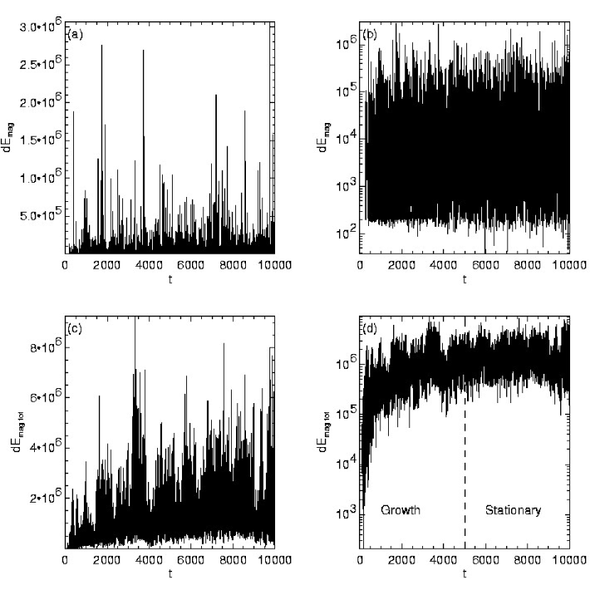
Figure 2: Initial growth of energy dissipations for parameters $\langle\textrm{a}\rangle$ (see Table 1): magnetic energies dissipated in the whole simulation box (a and b) and in one given plane (c and d) are plotted for the 10 000 first time steps of the simulation. a) and c) have linear coordinates, b) and d) have semi-logarithmic coordinates. Note that no magnetic energy is dissipated in the box until $t=90$, and in the plane until $t=240$. Note also that a stationary state is reached from $t\approx 5000$ (bottom right).

Histograms and fitting methodology.

The heights of the bars of the histograms we plot are normalized by their width and they are are divided by the number of events, i.e. our histograms are empirical PDFs. A least-squares linear fit is then performed in bi-logarithmic axes, on a range determined by visual inspection of the histogram (see Figure 3b). This gives error bars on the slope of the linear fit, which is the slope of the expected histogram power-law. However, we should keep in mind that the choice of the fitting range often introduces much larger error bars (typically $\pm 0.1$ to $0.2$) than the error bars of the least-squares linear fit of the slope (typically $\pm 0.01$ to $0.05$). The error bars we give from now are conservative estimates taking into account the fitting range uncertainty.

Figure 3: Histograms of magnetic energy dissipations a) in the whole simulation box ; b) in one given plane. The dotted lines correspond to one event per histogram bar ($0.02$ decades wide each).

Choice of the variable used for the statistics and general shape of the PDF.

Former studies (Aletti et al. (2000); Aletti (2001)) plotted the histograms or PDFs of the magnetic energy dissipation $\Delta E_{\textrm{\scriptsize tot}}$ calculated in the whole simulation box (Fig. 3). The global shape of the PDF was a Gaussian. A power-law $\Pr(\Delta E_{\textrm{\scriptsize tot}})\propto\Delta E_{\textrm{\scriptsize tot}}^{-6}$ seemed to appear as a deviation from the Gaussianity in the tail of the distribution, but it only spanned half a decade, which makes it perhaps not so relevant. On the contrary, we choose to plot the PDF of the magnetic energy $\Delta E_{i}$ dissipated in one given plane $i\in[1,N_{L}]$ (Fig. 3b). As the computations are done in the Fourier space, this is our primary variable. The power-law that can be fitted to the PDF of this variable has a much wider range (more than $2$ decades) and is much less steep (the index is between $1$ and $2$) than in the former case.

This can be explained by a Central Limit Theorem after remarking that $\Delta E_{\textrm{\scriptsize tot}}=\sum_{i}\Delta E_{i}$ and that the $E_{i}$’s are quasi-independent (as expected, the correlation between fields in neighboring planes is very low), thus the PDF of $\Delta E_{\textrm{\scriptsize tot}}$ is the convolution of the PDFs of all $\Delta E_{i}$ for $i\in[1,N_{L}]$. The difference between the PDFs in both cases stresses the importance of the choice of the variable used for the statistics. It also emphasizes that in the case of the statistics of observational data, we have to be careful about the definition of an “event”.

Both distributions of $\Delta E_{i}$ and of $\Delta E$ show a maximum. In the case of $\Delta E_{i}$, it is a consequence of the finite range of the power-law distribution ; the position of the maximum depends the average event size and on the slope. In the case of $\Delta E$, knowing the distributions $\Delta E_{i}$ in all planes $i$, it can be seen as a simple consequence of the Central Limit Theorem.

Effect of initial growth on statistics.

During the initial energy growth, the PDF of the energy of events is different than during the stationary state. In particular, it is shifted to the left, i.e. the events are smaller. As a result, the left part of the PDF of events energy gets higher than what it would be if stationary state events only were taken into account, as seen on Fig. 4. As we are interested in stationary state events, we choose to exclude events occuring during the initial energy growth from the statistics.

Figure 4: Effect of initial energy growth on the statistics of magnetic energy dissipations in the entire box : one histogram (solid line) only takes into account stationary state events, whereas the other one (dashed line) also takes into account the events produced during the initial phase.

Typical fields.

As the model is built on phenomenological evolution rules, it is not expected that the fields produced by the simulation coincide with any real picture. However, as we have tried to be as close as possible to the original MHD equations it is interesting to see how far the fields are realistic and what the limits of this phenomenological model could be. Typical magnetic and current density fields for $\alpha=2$ and $\alpha=4$ are shown on Fig. 5. On both samples but especially for high values of $\alpha$, we can notice that high current densities occur in magnetic “islands” and in regions where magnetic field densities are high. We do not observe many structures such as current sheets or possible reconnection sites, as will be discussed in section 4.1, although they are more present for small values of $\alpha$. Large-scale photospheric forcing (large $\alpha$) leads to large-scale structures.

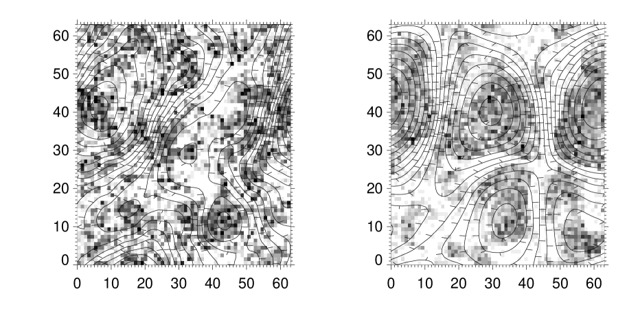
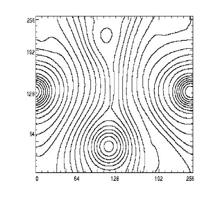
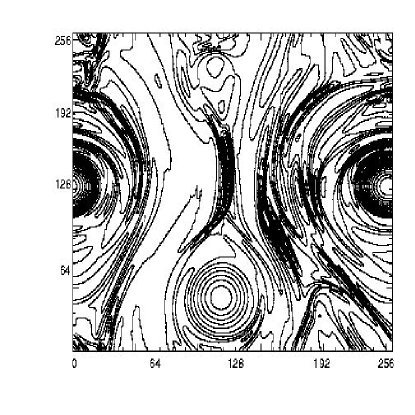
Figure 5: Top : magnetic and current density fields produced in a plane of the simulation box, for parameters sets $\langle\textrm{i}\rangle$ ($\alpha=2$, left) and $\langle\textrm{o}\rangle$ ($\alpha=4$, right). On both samples, the magnetic field lines are superimposed on a grayscale map of $J_{z}^{2}$ with large values in black. Bottom: magnetic field (left) and current density contours (right) issued from numerical integration of RMHD equations (courtesy Georgoulis et al. (1998)).

3.2 Parametric study of event energy PDFs

A parametric study is performed in order to explore the influence of the simulation parameters on the magnetic energy dissipations PDFs. A reference set of parameters, called $\langle\textrm{a}\rangle$, is chosen (see Table 1), and it gives the PDF shown on Fig. 3 . The PDFs obtained for other sets of parameters will be compared to the PDF obtained for $\langle\textrm{a}\rangle$. Most of the sets of parameters correspond to the modification with respect to $\langle\textrm{a}\rangle$ of one parameter (dissipation efficiency $C$, magnetic resistivity $\eta$, loading spectrum index), which is in italic in Table 1. All simulations were performed on $200\,000$ timesteps, which seems sufficient to achieve a long stationary state after the initial energy growth phase, and to achieve good statistics for the PDFs. Histograms were done with data from the $100\,000$ last timesteps.

Other parameters, which are not changed during the study, include the grid size (see above) and the current density threshold $J_{c}=300$. A higher grid resolution would have been interesting so as to get a broader wavelength range, but it would need a rescaling of other parameters and longer computation times. The current density threshold fixes the scale of current density, so its value has no intrinsic meaning.

Table 1: Sets of parameters used for the parametric study. $C$ is the dissipation efficiency, $\eta$ is the magnetic resistivity and $\alpha$ is the index of the 1D power-law loading spectrum. Parameters which are different from parameters set $\langle\textrm{a}\rangle$ are shown in italic font.

	$C$	$\eta$	$\alpha$
$\langle\textrm{a}\rangle$	$0.5$	$1\cdot 10^{-3}$	$5/3$
$\langle\textrm{b}\rangle$	$\mathit{0.1}$	$1\cdot 10^{-3}$	$5/3$
$\langle\textrm{c}\rangle$	$\mathit{0.3}$	$1\cdot 10^{-3}$	$5/3$
$\langle\textrm{d}\rangle$	$\mathit{0.7}$	$1\cdot 10^{-3}$	$5/3$
$\langle\textrm{e}\rangle$	$\mathit{0.9}$	$1\cdot 10^{-3}$	$5/3$
$\langle\textrm{f}\rangle$	$0.5$	$\mathit{3\cdot 10^{-4}}$	$5/3$
$\langle\textrm{g}\rangle$	$0.5$	$\mathit{3\cdot 10^{-3}}$	$5/3$
$\langle\textrm{h}\rangle$	$0.5$	$1\cdot 10^{-3}$	$\mathit{3/2}$
$\langle\textrm{i}\rangle$	$0.5$	$1\cdot 10^{-3}$	$\mathit{2}$
$\langle\textrm{j}\rangle$	$0.5$	$1\cdot 10^{-3}$	$\mathit{7/3}$
$\langle\textrm{k}\rangle$	$0.5$	$1\cdot 10^{-3}$	$\mathit{8/3}$
$\langle\textrm{l}\rangle$	$0.5$	$1\cdot 10^{-3}$	$\mathit{3}$
$\langle\textrm{m}\rangle$	$0.5$	$1\cdot 10^{-3}$	$\mathit{10/3}$
$\langle\textrm{n}\rangle$	$0.5$	$1\cdot 10^{-3}$	$\mathit{11/3}$
$\langle\textrm{o}\rangle$	$0.5$	$1\cdot 10^{-3}$	$\mathit{4}$

Dissipation efficiency.

Dissipation efficiency tells how much the system gets relaxed after a series of iterative dissipations : the current density threshold $J_{c}$ is replaced by a new threshold $C\cdot J_{c}$ after the first dissipation. With respect to the value $C=0.5$ used in parameters set $\langle\textrm{a}\rangle$, the dissipation efficiency can be set to almost any value of its range $[0,1]$ of valid values with almost no visible change in the PDFs.

Magnetic resistivity.

Magnetic resistivity $\eta$ could vary in the range $[3\cdot 10^{-4},3\cdot 10^{-3}]$. A numerical stability analysis, given the time step fixed to one and the wavenumber range, shows that higher values of $\eta$ would result in numerical instability. On the other hand, lower values of $\eta$ would lead to longer computational time. However, $\eta$ has mainly an influence only on the dissipation process length; a change in the value of $\eta$ has little influence on the histograms of dissipated energies.

Loading spectrum.

The reference parameters set $\langle\textrm{a}\rangle$ has a loading spectrum index $\alpha=5/3$, corresponding to the spectrum in the inertial range of Kolmogorov turbulence. In parameters sets $\langle\textrm{a}\rangle$ and $\langle\textrm{h}\rangle$ to $\langle\textrm{o}\rangle$, $\alpha$ varies from $3/2$ to $4$ by a maximal interval of $1/3$. Another series of simulations was performed with lower loading power values to explore the influence of the ratio $P_{\mathrm{load}}/J_{c}$. For both series, for high values of $\alpha$, the power-law is well defined (3 to 4 orders of magnitude wide). Its slope index is approximately $-1.6$, and this value depends neither on the loading spectrum index $\alpha$ (as seen in Table 2 and Figure 6, and as will be discussed in section 4.1) nor on the loading intensity $P_{\mathrm{load}}$. For low values of $\alpha$, however, power-laws were difficult to obtain, and their slopes were sensitive to both loading spectrum index and loading intensity.

Table 2: Variability of the event energy PDF power-law index $\zeta$ as a function of the loading spectrum index $\alpha$.

	$\alpha$	$\zeta$
$\langle\textrm{h}\rangle$	3/2	$1.64\pm 0.54$
$\langle\textrm{a}\rangle$	5/3	$1.57\pm 0.57$
$\langle\textrm{i}\rangle$	2	$1.61\pm 0.33$
$\langle\textrm{j}\rangle$	7/3	$1.71\pm 0.27$
$\langle\textrm{k}\rangle$	8/3	$1.76\pm 0.07$
$\langle\textrm{l}\rangle$	3	$1.65\pm 0.02$
$\langle\textrm{m}\rangle$	10/3	$1.63\pm 0.03$
$\langle\textrm{n}\rangle$	11/3	$1.61\pm 0.01$
$\langle\textrm{o}\rangle$	4	$1.61\pm 0.01$

Figure 6: Event energy PDF power-law index $\zeta$ as a function of the loading energy spectrum index $\alpha$ (Table 2). On the left, the big error bars are a consequence of the fact that the fitting range is not well defined.

3.3 Statistics of durations of events

Durations of events extend over two decades. They are indeed a discrete variable, which is a multiple of the cascade time step $\delta t_{c}$, and their maximum value is a few hundreds times $\delta t_{c}$. Histograms can be obtained, although their width is too narrow to perform relevant power-law fitting (see figure 7).

The duration of an event is correlated with its energy, like $dE_{i}\propto dt_{i}^{1.76}$, as seen on the scatter-plot on figure 8. Another way to visualize this correlation is to select events according to their duration, and to plot the histogram of energies of events from this population, as shown on figure 9. One possible observational consequence could be that missing long-duration events, due for example to short observation times, can lead to energy histograms with narrower ranges and steeper slopes.

Figure 7: Histogram of events durations for parameters set $\langle\textrm{l}\rangle$.

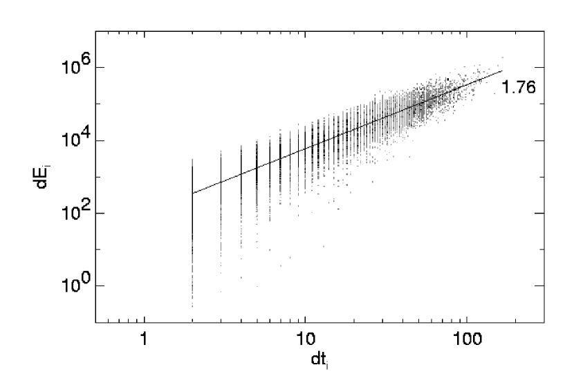
Figure 8: Correlation between events duration and energy for parameters set $\langle\textrm{l}\rangle$.

Figure 9: Event energy histograms for different event durations ranges, which form a partition of the whole duration range, from low duration (left, dashed) to long duration (right, dashed). The sum of these histograms (i.e. the event energy histogram of all events as in figure 3b) is shown as a solid line.

4 Discussion and Conclusions

4.1 Properties of the model

The CA model presented here differs from previously presented work in two features. On the one hand, the energy pumping due to photospheric motion is known quite accurately via solution of the Alfvén wave propagation equation with reflecting boundary conditions. Each cell therefore receives and sends energy to neighboring cells along the loop axis via a wave equation. Energy redistribution to cells on the same loop plane however occurs using an instability and redistribution criterion. This criterion is a threshold in current, and satisfies the basic requirements for magnetic fields of divergence-free conditions and realistic current redistribution.

Power-law slope of energy distributions as a function of parameters.

When parameters sets lead to wide and robust power-law statistics of events energies, it seems that the slope of these power-laws is quite the same and takes a value close to $-\zeta=-1.6$. If this behavior is confirmed by further parametric studies, it could be interpreted as the “universal” behavior of SOC systems, described for example in Bak et al. (1987).

It is however interesting to note that Georgoulis & Vlahos (1998) observe in their model a variability of the slope of event energy (and also peak luminosity and duration) as a function of the loading : the slope is steeper when the amplitude distribution of the loading increments has a steeper power-law. However, this discrepancy is due to the differences in the way the system is driven : their loading increments are discrete in space whereas our loading has a varying spatial spectrum and no power-law amplitude distribution variation.

Reconnection, and the quality of the dissipation criterion.

Snapshots of the superposition of the magnetic lines with the current densities (see figure 5) reveal that the sites of dissipation often do not correspond to reconnection of magnetic field lines ; the reason is that one may have intense currents (and our dissipation criterion is based precisely on current intensity) without having a topology of the field where reconnection occurs (instabilities such as resistive kinks and/or tearing modes are triggered by a combination of currents and current gradients). Though the typical field structures observed resemble fields from turbulence simulations, one sees that our simplified model distributes dissipation in a different, more homogeneous way. Of course, a cellular automaton model, which models the non-linear terms of the equations through simple threshold dynamics, is not supposed to generate such structures, but we can try to understand what can be done to improve the model. The physical quantities available in our model make it for example possible to use a more elaborate dissipation criterion which would model more accurately the reconnection instability threshold, such as for example introducing a combined criterion on current and current gradients as a trigger for relaxation.

4.2 Comparison with observations

Impulsive coronal events are statistically distributed over an energy range of some eight orders of magnitude. Since Parker’s idea of the existence of nanoflares, it has been thought that at some point in the quest of small scale coronal structures we will break the self-similarity of the solar corona by the observation of a steepening of the flare distribution with finally a power-law index $\zeta$ greater than the critical value of $2$. Recent data analyses (Krucker & Benz, 1998; Aschwanden et al., 2000; Parnel & Jupp, 2000) seem to show this behavior with observed values of $\zeta$ going up to $2.6$. Empirical formulas have been used here to determine flares energies from observed luminosities but new analyses of the data (Aschwanden & Charbonneau, 2002; Benz & Krucker, 2002) reveal in fact the existence of a bias due to the finite range of temperature on which the observations are made. The correction of this temperature bias leads eventually to a value of $\zeta$ close to $1.6$ valid for the whole range of energies, from unresolved, X-ray observations with the Solar Maximum Mission (SMM) to Extreme Ultra-Violet observations with the Extreme-Ultraviolet Imaging Telescope on the Solar and Heliospheric Observatory (SoHO/EIT) and the Transition Region And Coronal Explorer (TRACE) – see Aschwanden et al. (2000). Such an observational bias, as well as the one described in the end of paragraph 3.3, show the importance of defining well what an event is and what its characteristics are, when observing the corona but also when using statistical flare models.

The comparison between model distributions and observed distributions is actually not an easy task, even if it is tempting to compare the power-law slope $1.6$ obtained by our model to the observed global slope of $1.6$. The first pitfall for comparison between statistical results of observations and models may be linked to the spatial resolution of observations ($\approx 100\>\mathrm{km}$ at best) compared to the dissipative scales of the system ($\approx 100\>\mathrm{m}$). It is clearly shown in this paper that the plot of the PDF of the magnetic energy dissipated in a given plane of the model has a shape quite different from the PDF of the same observable but for the whole simulation box. The bias here consists of a steepening of the power-law slope with an index greater than $2$. This result suggests that the limited instrumental resolution may be a source of error as well. The SOHO/EIT observations analyzed by Aletti et al. (2000) seem to illustrate quite well this interpretation : the pixel intensity distribution power-laws are steeper (with indices going up to $5.6$) at lower resolution. Most of the coronal structures in the quiet Sun are indeed smaller than the spatial resolution of EIT. Besides, the domain where the power-law is fitted on the PDF is reduced which leads to larger error on the value of the index. Reliable statistical results could be accessible with higher instrumental resolution but also by using mathematical tools like for example Pearson’s method (Podladchikova, 2002).

However, we think that resolution has not always such a dramatic effect on the slope of the PDFs, and that it is still interesting to model statistics of individual events (i.e. in one plane, in the case of our model). The convergence to a Gaussian when summing the energies of events before doing statistics, predicted by an argument lying on the Central Limit Theorem, may indeed be much slower in the case of observed, real micro-events than in the ideal case of independent events with low-moments distributions: the distributions of real events energies are much wider than the modeled distributions and their moments may be greater. As a result, depending on the observational conditions, there could still exist a quite wide power-law after summation (due to lack of resolution) of a large but not too large number of events, and the slope of this distribution may be still close to the slope of the original distribution of individual events. In this context the slope $\zeta=1.6$ we obtain is rather encouraging.

Another prediction of our model is that durations and energies of events scale like $dE_{i}\propto dt_{i}^{1.76}$, or, equivalently, $dt_{i}\propto dE_{i}^{1/1.76}=dE_{i}^{0.57}$. This exponent $0.57$ is in quite good agreement with Berghmans et al. (1998), who report that observed events durations scale like their radiative loss at the power $0.5$.

We should however emphasize that statistical flare models usually give energy dissipations, while observations give luminosities at some given wavelengths and the infered energies depend on models. It is therefore crucial in the future to develop models including the production of observable quantities, in order to provide stronger links between models and observations but also to quantify more precisely the weight of observational biases. The first agreements obtained during the last decade between statistical predictions made by theoretical models and observations are however very promising.

4.3 Summary and conclusion

In this paper we have presented a three-dimensional simplified model inspired by the RMHD equations whose first version was introduced by Einaudi & Velli (1999). This model mimics a coronal magnetic loop anchored in the photosphere whose footpoints are driven randomly by convective motions. The slow driving of the magnetic footpoints leads to storage of energy along the coronal loop and eventually to dissipation through impulsive events. The characteristics of the model are the following : (i) the model describes Alfvén wave propagation along a loop exactly ; the internal structure of the loop is described by a set of planes distributed along the axis and ending in the photosphere from which the information propagates ; (ii) the external forcing applied to the two boundary planes is expressed as a turbulent spectrum in Fourier space ; (iii) when the criterion of instability is satisfied, the dissipation of current density and vorticity takes place non-locally in Fourier space but still locally in physical space ; (iv) Fast Fourier Transforms (FFT) are implemented in the numerical code to use the dual physical/Fourier space.

A numerical study has allowed to quantify the role of the parameters, especially forcing, in the behavior of this model and in statistical properties of coronal events. The slope of event energy histograms was found to be almost constant, in accordance with a SOC-like “universal” behavior, and consistent with the values given by observations. Event durations statistics were performed, and correlations with event energies are also compatible with observations. Different possible observational biases were pointed out, all of them resulting in a narrower power-law range on histograms and in a steeper slope than in the statistics of all elementary events : a bias due to the limited spatial resolution, which gives a possible interpretation of recent observations made with the instrument EIT on board SoHO, and a bias due to limited observation durations.

Improvements are always possible to provide a better description of the physics. One can imagine some ad-hoc rules to obtain for example a correct picture of the reconnection process. But the probably most interesting (and difficult) study is about the incorporation of the non-linear dynamics in a more realistic way than the simple on-off mechanism of CA models, but without going directly to the MHD equations. From a pure observational point of view it seems crucial to have as precise as possible an estimate of the possible biases to determine the effective value of the power-law index $\zeta$ of the energy distribution. Indeed the confirmation of the sub-critical value of $\zeta$ could be a serious challenge to Parker’s hypothesis of coronal heating by a swarm of nanoflares.