Automatic abundance analysis of high resolution spectra

We describe an automatic procedure for determining abundances from high resolution spectra. Such procedures are becoming increasingly important as large amounts of data are delivered from 8m telescopes and their high-multiplexing fiber facilities, such as FLAMES on ESO-VLT. The present procedure is specifically targeted for the analysis of spectra of giants in the Sgr dSph; however, the procedure may be, in principle, tailored to analyse stars of any type. Emphasis is placed on the algorithms and on the stability of the method; the external accuracy rests, ultimately, on the reliability of the theoretical models (model-atmospheres, synthetic spectra) used to interpret the data. Comparison of the results of the procedure with the results of a traditional analysis for 12 Sgr giants shows that abundances accurate at the level of 0.2 dex, comparable with that of traditional analysis of the same spectra, may be derived in a fast and efficient way. Such automatic procedures are not meant to replace the traditional abundance analysis, but as an aid to extract rapidly a good deal of the information contained in the spectra.

Figure 1: Example of fit to a simulated noisy spectrum. The thin line is a synthetic spectrum corresponding to T${}_{eff}=5000$ K, log g = 2.50, [Fe/H]=–0.5, [$\alpha$/Fe]=+0.4, $\xi=1.0{\rm kms^{-1}}$ and pseudo-normalized as described in the text. The thicker line is the same spectrum in which noise has been injected so that S/N = 10 and pseudo-normalized after the injection of noise. The two vertical lines delimit a pseudo-continuum window. The two thick lines are the fitted spectra of two Fe i features.

Figure 2: Optical depth as a function of temperature for three models with T=4750 K and log g=2.5. The solid line corresponds to a model with [M/H]=–0.5 and [$\alpha$/Fe]=0.0 and the dashed line to one with same [M/H] and [$\alpha$/Fe]=0.4; the dotted line corresponds to a model with [M/H]=–0.19 and [$\alpha$/Fe]=0.0. In the inset is shown a zoom of the temperature structure of the models at large optical depths. A difference of about 60 K between the model with [M/H]=–0.5, [$\alpha/Fe$]=0.4 and the model with [M/H]=–0.19, [$\alpha/Fe$]=0.0 can be appreciated.

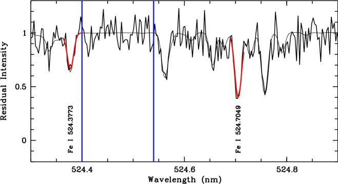
1 Introduction

In recent years considerable attention has been devoted to full or partial automation of the process of abundance determination from high resolution spectra (Katz et al., 1998; Katz, 2000; Erspamer & North, 2002a, b). One of the main thrusts behind these attempts is the increasingly large amount of data delivered by modern instrumentation. It is well known that astronomical archives are full of good quality high resolution spectra which have not been analysed, or only partially analysed, due to lack of manpower. In spite of the complexity of data reduction, this is not the bottleneck, thanks to the efficient software and instrument-dedicated pipelines that are available. The real bottleneck is the data analysis which, for abundances, is still done more or less in the same way as twenty years ago. The situation is going to become even more critical as high-multiplex instruments, such as FLAMES on ESO-VLT (Pasquini et al., 2000), become fully operative.

In the last years we have devoted special interest to the determination of abundances in giants of the Sgr dSph (Bonifacio et al., 1999; Bonifacio, 1999; Bonifacio et al., 2000). Such an astrophysical problem is ideal for the capabilities of FLAMES. It has also the advantage that two of the key parameters in the interpretation of stellar spectra, effective temperature and surface gravity, may be conveniently constrained. If we pick stars of roughly the same apparent magnitude, if they belong to Sgr, they will have the same luminosity and therefore surface gravity. At a given luminosity the RGB of Sgr spans a limited range in effective temperature, in fact less than 1000 K, and in the case of our sample less than 250 K. We had already attempted to develop a procedure to analyse the low resolution spectra which we obtained from EMMI-NTT (Bonifacio et al., 1999; Bonifacio, 1999), however the procedure, based on spectral indices, provided unsatisfactory results, essentially because of the combination of low resolution and low S/N ratios. Furthermore it was apparent that at low resolution we had no handle on the microturbulent velocity, and since the abundances relied only on strong lines (the only ones available at low resolution, whichever the S/N ratio), the result was strongly dependent on the unknown microturbulent velocity. Having in mind the future use of FLAMES and having available a few UVES spectra, obtained in slit-mode, we decided to concentrate on a procedure capable of analysing spectra from UVES and Giraffe. We have developed a procedure which is very efficient and stable, at least on the real UVES spectra. In spite of the fact that it is highly targeted (it will deal only with stars of a given luminosity and a limited range of effective temperatures), it has been written in such a way that it may be modified to deal with other types of stars. In this paper we describe the procedure placing our emphasis on the algorithms and on the stability of the method. The procedure rests on synthetic spectra computed from 1D LTE model atmospheres. In this paper we do not question the reliability of the input synthetic spectra, since it is straightforward to replace the existing grid with a better one, when available.

Table 1: Algorithm meta-code

BEGIN
	$\xi$;
		pseudo-normalize;
		find [Fe/H] for each FeI feature;
		find slope A(FeI) vs. EW;
		if slope$<$ threshold, go to $\alpha$;
		find a $\xi$ to make slope smaller;
	goto $\xi$;
	$\alpha$;
		find [Mg/H] for each Mg I feature;
		find [Ca/H] for each Ca I feature;
		[$\alpha$/Fe] = mean of [Mg/Fe] and [Ca/Fe];
		if $\Delta$[$\alpha$/Fe] $<$ threshold1 goto END;
	goto $\xi$;
END

Figure 3: Histogram of the derived [Fe/H] for Monte Carlo simulations with different S/N ratios and a resolving power of 7 kms^-1

Figure 4: Monte Carlo simulations corresponding to a resolving power of 7 kms^-1: [Fe/H], [$\alpha$/Fe] and microturbulence velocity as a function of S/N for input spectrum at $\xi=1.$Km/s, [$\alpha$/Fe]=0.4 and [Fe/H]=–0.5 on the left panel and [Fe/H]=–1.5 on the right panel. For both the [Fe/H] vs S/N plots the smaller error bars correspond to Monte Carlo simulation dispersion, the bigger one to the [Fe/H] dispersion over the all Fe i features.

Figure 5: Comparison of [Fe/H], [$\alpha$/Fe] and $\xi$ from the traditional analysis and the automatic analysis for the 12 stars of Sgr observed with UVES. The left panels display the results from the UVES spectra, i.e. at a resolving power of $\sim 7\rm kms^{-1}$; the right panels display the results from the UVES spectra convolved with a gaussian profile, obtaining a resolving power of $\sim 20\rm kms^{-1}$. The two points, in each of the eight panels, shown as crossed squares, identify the two stars for which the log g adopted in the traditional analysis is not 2.5.

Figure 6: Comparison of [Fe/H], [$\alpha$/Fe] and $\xi$ obtained for the 12 Sgr giants observed with UVES directly from the UVES spectra (resolving power $\sim\rm 7kms^{-1}$) and UVES spectra broadened to a resolving power of $\sim\rm 20kms^{-1}$.

2 Algorithms

The algorithms employed by our code reproduce those usually employed in abundance analysis of stellar spectra. The whole procedure rests on the comparison between computed and observed spectra. We assume that the observed spectra have been fully reduced and shifted to rest-wavelength. For the Giraffe spectra it is expected that the instrument pipeline will provide radial velocities through cross-correlation. The basic algorithm of our code is summarized as meta-code in Table 1.

2.1 Pseudo-normalization

The first step is the normalization of the spectra: this is done by defining a set of continuum windows. In each window the continuum is defined as a quasi-median: if there are $N$ pixels in the window the pixels are sorted by number of counts; let $n=[3N/5]$, the continuum is defined as the number of counts in the $n-$th pixel. This definition was chosen because extensive Monte Carlo simulations showed that it performed better than the median. The point in the (wavelength, counts) plane defined by the central wavelength and this quasi-median of the continuum window is considered as a continuum, or rather pseudo-continuum, point. A spline is then passed through these points and the spectrum pseudo-normalized dividing it, pixel by pixel, by this spline. It is impossible to define true continuum windows, each one is affected by weak absorptions, which are larger the lower the effective temperature and the higher the metallicity. In Fig. 1 we show an example of a typical continuum window and of pseudo-normalized spectra in a simulation with a synthetic spectrum. In order to make a meaningful comparison the computed spectra are normalized (or pseudo-normalized, to be rigorous) exactly in the same manner as observed spectra. One could fear that the synthetic and the observed spectrum are not normalized exactly in the same way, since the observed spectrum may have a complicated shape due to variations of the instrumental efficiency (CCD QE, blaze function and, in the case of Giraffe, transmission of the order-separating filters). To avoid these problems, the continuum windows on the one hand must be small enough that the instrument response function $\cal R$ is constant in the window. In this case the pseudo-normalized spectrum in the window is $F_{\lambda}{\cal R}/<F_{\lambda}{\cal R}>\sim F_{\lambda}/<F_{\lambda}>$, where $F_{\lambda}$ denotes the incoming photon flux and the angle brackets denote the quasi-median. It is thus approximately independent of the instrument response function. On the other hand there must be enough pseudo-continuum windows to capture the variations of the instrument response function. It is clear that the width and number of pseudo-continuum windows must be chosen also to satisfy these requirements and is therefore instrument-dependent. In the case of the UVES data the instrument response function is very smoothly varying. Our chosen continuum windows have widths $w$ in the range $0.05{\rm nm}\la w\la 0.4{\rm nm}$ and the distance $d$ between windows is in the range $0.1{\rm nm}\la d\la 3.0{\rm nm}$ with an average $d\sim 1$nm. It is possible that, when we have at our disposal true Giraffe data, we shall have to revise the continuum windows. However one must keep in mind that, in the process of data reduction prior to the analysis, one tries to remove the instrument response function as well as possible (“rectify” the spectra), and one is left with a trend which is smooth and well approximated by a spline. With UVES spectra this is very well achieved over intervals of $\sim$ 20nm such as we are considering. Inspection of Fig. 1 suggests that the correct position of the pseudo-continuum is recovered even at very low S/N levels.

Since our work is specifically targeted to the study of giants in the Sagittarius dwarf Spheroidal using the FLAMES facility, our program presently runs assuming that two spectral ranges, corresponding to high resolution settings HR09 and HR14 of the Giraffe spectrograph, are available. These were chosen in order to give information on Fe, the $\alpha$ process elements Ca and Mg, as well as Si, Ti, the iron peak elements Sc, V and Ni, and the n-capture elements Ba and La, thus providing information on three distinct nucleosynthetic channels. In the present paper we focus on the Fe, Mg and Ca, however extension to all the other available elements is under way and some results are presented in section 5.2.

2.2 Selected spectral features

A number of spectral regions are selected, each one is dominated by one line of a given ion. In Fig. 1 two typical Fe i features used are labeled and the fitted profiles are shown. In the following we refer to these as features and not lines, since, although dominated by a line, they are affected by several blending lines whose relative importance changes with atmospheric parameters. These windows have been optimized for a resolution of 7 $\rm kms^{-1}$, relevant to the UVES data on which the procedure has been tested. At the lower resolution of Giraffe these windows change slightly. For each range a comparison between the Kurucz, Furenlid, & Brault (1984) solar atlas and a synthetic spectrum computed from the Kurucz solar model (Kurucz, 1993) has been done in order to check the considered features. We have rejected some features, which were very poorly reproduced by the synthetic spectrum. However, for some of the features which we retained, the discrepancies between synthetic and observed spectrum are not negligible. Had we rejected all of these, we would have been left with too few features to base our analysis on. A possibility would have been to modify the atomic data used for computing our synthetic spectra, in order to force a good fit of the solar spectrum, as done, for instance by Chavez, Malagnini, & Morossi (1997). However since the stars in Sgr, which we want to study, have temperature, gravity and, perhaps, metallicity very different from the Sun, there is no guarantee that changes to the atomic data made to obtain a better fit in the Sun will ensure also a better fit in our stars. Moreover it is not obvious how much of the disagreement is due to the atomic data and how much to the temperature structure of the model atmosphere (see for example Grevesse & Sauval, 1999). Therefore rather than introducing ad hoc changes, whose effect is difficult to predict, we prefer to keep features for which our capability to reproduce the solar spectrum is less than optimal and validate our procedure by comparing the results with that of a traditional abundance analysis, based on different lines.

2.3 Fitting observed features

The comparison of observed and synthetic spectra relies on least-square fitting. For each region we define $\displaystyle\chi^{2}=\sum\left({O_{i}-S_{i}\over\sigma}\right)^{2}$ where $O_{i}$ is the observed spectrum for the $i-th$ pixel, $S_{i}$ is the synthetic spectrum and $\sigma$, assumed equal for all pixels, is defined as $\displaystyle\left[{1\over 2}\left({<C_{l}>\over\sigma_{l}}+{<C_{r}>\over\sigma_{r}}\right)\right]^{-1},$ where $<C_{l}>$ and $<C_{r}>$ are the mean number of counts in the nearest continuum windows to the left and to the right of the given feature; $\sigma_{l}$ and $\sigma_{r}$ are the standard deviations in the same. At each step in the code the fitting of any feature has two parameters: the abundance and a small shift in central wavelength of up to one resolution element. Since the fit is done on each line separately this is specific to each spectral window and not a global shift. The minimum $\chi^{2}$ is sought numerically using MINUIT (James, 1998). Two comments are in order here:

1. The theorems on the statistical properties of the $\chi^{2}$ are not applicable in the case of real spectra. If the spectra have been rebinned to a constant wavelength step, as is usually done, the neighbouring pixels are obviously correlated. This is however true also for non-rebinned spectra; since the slit width normally projects onto several pixels, thus adjacent pixels belonging to the same resolution element are correlated.

2. The assumption that all pixels have the same $\sigma$ is acceptable for weak lines but it clearly breaks down for a strong absorption line, whose central residual intensity is near to zero.

In spite of this, our Monte Carlo simulations show that $\chi^{2}$ fitting may be used to determine the correct values of the fitting parameters (in our case abundances) and the error on the fit may be conveniently estimated using Monte Carlo simulations. On the other hand the ”goodness of fit” derived from the $\chi^{2}$ distribution may have little meaning in an absolute sense. However we need some way to discriminate between “good” and “bad” fits in order to reject the latter. Our pragmatic solution is to use the formal “goodness of fit” but to consider the minimum probability to accept a fit to be a free parameter which must be tuned to the actual data to be analysed, based on the results of Monte Carlo simulations and, when available, on the results for stars of known abundance.

2.4 Fitting parameters

Given that computing synthetic spectra is time consuming, these are pre-tabulated in a spectrum library, and linear interpolation is used when necessary. We assume that the effective temperature and the surface gravity of the star are known. The Sgr giants, we are interested in, have more or less the same gravity and effective temperature may be derived e.g. by a suitable colour such as (V–I). We shall estimate the errors due to incorrect choice of temperature or gravity. As detailed in the next section, our synthetic grid is based on standard, flux constant, plane parallel model atmospheres computed with the ATLAS 9 code. Therefore the atmospheric parameters to be estimated are: metallicity, which we define for practical reasons to be [Fe/H], the microturbulent velocity and the $\alpha$ enhancement. The latter parameter is often neglected in abundance analysis. In fact it is customary to neglect the effect of chemical composition on the atmospheric structure. While this is acceptable for trace elements, such as Li, it is not acceptable for the $\alpha$ elements, at least for the most metal-rich models.

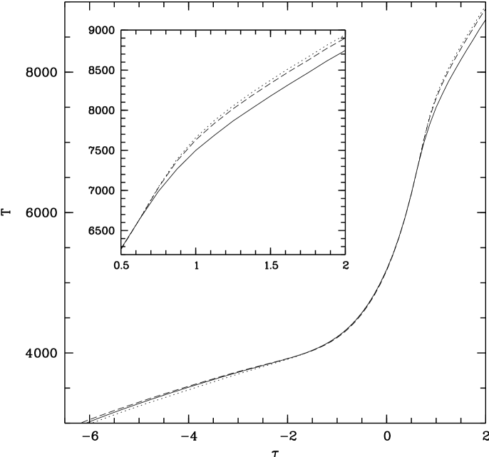
As an example we show in Fig. 2 the run of temperature vs Rosseland optical depth for three models with the same effective temperature, gravity and microturbulence. The solid line and the dashed line correspond to [M/H]$=-0.5$ and [$\alpha$/Fe]=0.0 and +0.4 respectively. The differences at large optical depths, where weak lines are formed, are as large as 200 K as shown in the inset. Apart from the different temperature structure of the models the abundance of $\alpha$ elements has a direct impact on the pseudo-continuum, especially in the region from 510 nm to 525 nm, which is filled by weak MgH lines, which affect also the continuum windows. In reality one should not label the models by their value of [Fe/H], but rather by their Z. The model with [M/H]=–0.5 and [$\alpha$/Fe]=0.4 has Z=0.0061; the model with the same [M/H], but [$\alpha$/Fe]=0.0, has Z=0.0126. Therefore a model with [$\alpha$/Fe]=0.4 and [M/H]=–0.5 has about the same Z as a model with [$\alpha$/Fe]=0.0 but [M/H]=–0.19 (to be precise a model with [M/H]=–0.186 has Z=0.0126). We calculated such a model using an appropriate ODF and found that, although the Z is the same, the temperature structure of the two models still differs in depth by about 60 K as shown in Fig. 2. Therefore, although Z is a better description of the overall properties of the model than [Fe/H] or [M/H] and [$\alpha$/Fe] the details still depend on the precise chemical composition. Moreover in order to know Z one must know the abundances of all elements, or, at least C, N and O, which, in general, are quite difficult to obtain. On the contrary [Fe/H], [Mg/H] and [Ca/H] are relatively easy to obtain, it is thus not surprising that for practical reasons, when studying stellar spectra, the chemical composition is more conveniently described in terms of [Fe/H] and [$\alpha$/Fe] rather than Z.

2.5 Iterative steps

As outlined in the meta-code in Table 1 after the normalization of the spectra the next step is to determine the metallicity by fitting the Fe i features, in the above defined sense. For each feature the equivalent width (EW) is determined by trapezoidal integration of the fitted synthetic profile. Then the slope in the plane (log (abundance), log EW) is found. The computation is repeated for at least two values of the microturbulence $\xi$. The Fe i abundances are re-determined with the new microturbulence and the process is iterated until the residual slope is below a chosen value (experience has shown that a value like 0.001 log[EW(nm)]/dex is a good choice in practical cases). A possible concern is that in this step we are treating our features as if they were isolated lines. Suppose a feature were composed by many weak Fe i lines. It would be insensitive to microturbulence, since all the lines are on the linear part of the curve of growth. Yet its equivalent width could be large. The presence of several such features would force a small microturbulence velocity, when a higher one would be required. In practice one has to avoid such cases. We selected our features so that they behave, with respect to the microturbulent velocity, in the same way as isolated lines would do. Having fixed the microturbulence, the $\alpha$ to iron ratio is determined by fitting Mg and Ca lines. Once a value of [$\alpha$/Fe] is found, the process is iterated, as shown in Table 1, starting from Fe abundances, through determination of microturbulent velocity and a new value of [$\alpha$/Fe], until the change in [$\alpha$/Fe] is smaller than a chosen value (0.01 dex has been used in practical cases). Readers familiar with abundance analysis will recognize that this whole procedure is identical to what is used in traditional “fine abundance analysis”, except that in the latter isolated lines, rather than features formed by line blends are used. Moreover often effective temperature is adjusted to satisfy excitation equilibria and surface gravity to satisfy ionization equilibria. It would be in fact straightforward to implement these in our automatic scheme, however we reckon these adjustments are not important in the case of Sgr giants and prefer to simply estimate the error in abundances due to an incorrectly chosen temperature and gravity. Once metallicity, microturbulence and [$\alpha$/Fe] are fixed, the procedure can continue by determining the abundances of other available elements by fitting the relevant spectral features.

2.6 Stars with enhanced C and N abundances

Although so far none of the Sgr giants has been found to have enhanced CN bands, such stars are known to exist among field and globular cluster giants. The chosen spectral regions are characterized by the presence of many CN lines which are very weak in the case of solar or solar-scaled chemical compositions, however they become strong in the presence of very large enhancements of C and N. Such stars, if present, cannot be dealt with by the present procedure. We therefore identified a number of windows to be used as “CN alert”. These are regions characterized by very weak CN and/or CH lines, in the case of solar or solar-scaled chemical composition, which become appreciable in the case of conspicuous CN enhancement. We compute the absolute difference between the observed spectrum and the “best fitting” spectrum and use this and a user-defined threshold to set a “suspect CN” flag, which should prompt for further inspection of the spectrum. Tests with synthetic spectra have shown that we can discriminate against CN enhancements of [C/Fe] $\geq+0.4$ and [N/Fe]$\geq+0.4$. The C and N enhancements observed in C-rich N-rich stars are often much larger than this.

3 Grid of synthetic spectra

The synthetic spectra employed have been computed from LTE model atmospheres computed with the ATLAS code, using the SYNTHE code (Kurucz, 1993). The spectra cover the ranges corresponding to settings HR09 and HR14 of the Giraffe spectrograph. The grid covers 5 effective temperatures (4500 K, 4750 K, 5000 K, 5250 K, 5500 K), 5 metallicities ([M/H]=–2.0, –1.5, –1.0, –0.5, 0.0), two values of $\alpha$ enhancement (0.0, +0.4) and three microturbulent velocities ($\xi=1.0,\leavevmode\nobreak\ 2.0,\leavevmode\nobreak\ 3.0$ kms^-1) for a single value of log g = 2.5, thus it presently consists of 150 spectra for each of the above ranges. In the future the grid may be extended.

In the course of the fitting procedure the spectra are convolved with an instrumental profile and rebinned in wavelength in order to have the same step as the observed spectra. So far the procedure has been tested only on UVES data (R$\sim$ 40000) and on UVES data degraded to the expected resolution of Giraffe (R$\sim 15000$). The referee, P. North, pointed out that the high resolution mode of Giraffe, tested during the commissioning of the instrument, is higher than expected and in fact around 20000. To verify the impact of the increased resolution we performed a small set of Monte Carlo simulations also at this resolution, as detailed in the next section.

4 Monte Carlo simulations

4.1 Stability of the method

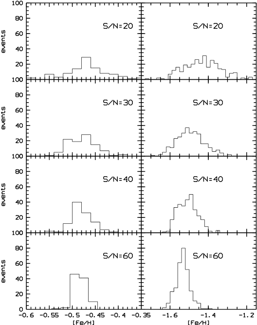
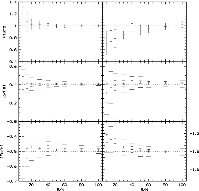
In order to estimate the stability of the method we resorted to Monte Carlo simulations. We took two synthetic spectra, with T = 5000 K, [$\alpha$/M]=+0.4, $\xi=1.0$ kms^-1 and metallicities [M/H]=$-0.5$ and $-1.5$. These were convolved with a Gaussian instrumental profile of 7 kms^-1 (to simulate a UVES spectrum) of 20 kms^-1 and a few also of 15 kms^-1 (to simulate a Giraffe spectrum). We injected Gaussian noise in order to reach various levels of S/N ratio (10, 15, 20, 30, 40, 50, 60, 80, 100) and ran the procedure for 300 MC samples in each case. For the resolution of 15 kms^-1 only S/N ratios of 20, 30, 40, 60, 80 were simulated. We verified that after about 300 samples the dispersions stabilized so as to make it unnecessary to run a larger number of samples. The histograms of the derived metallicity in the case of a resolving power of 7 kms^-1 are shown in figure 3. As expected the dispersion increases quite rapidly with decreasing S/N, however the dispersion at S/N = 20 is only about 0.05 dex. This is an “internal” error of the method and does not take into account systematic errors due to shortcomings of the synthetic grid (errors in the atomic data, inadequacy of model-atmospheres…) nor due to an incorrect choice of temperature or gravity. Furthermore the assumption of Gaussian noise is seldom a satisfactory one for real spectra, which are affected by cosmic ray hits, sky emission lines, and other sources of non Gaussian noise. Therefore our Monte Carlo simulations provide a check on the stability of the method, rather than an estimate of the accuracy of our procedure. Moreover in a practical case it is not straightforward how the S/N ratio should be estimated. Instead the dispersion of abundances derived from different features is a readily available parameter, which we suggest to use as error estimate. The Monte Carlo simulations show that this dispersion is always within a factor two of the Monte Carlo error, thus making it a suitable, although somewhat conservative, error estimate (see fig.4).

It is interesting to notice in Figures 3 and 4 how going to lower S/N ratios, the estimated metallicity shifts systematically to-wards higher values, although by a relatively small amount: for the simulations with [Fe/H]=–1.5 going from S/N=60 to S/N=20 the estimated metallicity increases only by about 0.1 dex. For the simulations with [Fe/H]=–0.5 the increase is negligible.

We estimated the error introduced by an incorrect choice of temperature and gravity by feeding to the procedure noise injected synthetic spectra with $T\rm_{eff}$= $\pm 100$ K and log g = $\pm 0.5$ dex . The corresponding changes in metallicity and $\alpha$ enhancement are $\pm 0.1$ dex and $\pm 0.04$ dex respectively for a 100 K change in $T\rm_{eff}$ and $\pm 0.04$ dex and $\mp 0.10$ dex respectively for a change of $\mp 0.5$ dex in log g.

The Monte Carlo simulations also provide a way of assessing the effect of the different resolutions. We ran Monte Carlo simulations on a noisy synthetic spectrum with [Fe/H]=–0.5, [$\alpha$/Fe]=+0.4, $\xi=1.0\rm kms^{-1}$ and S/N=20 with resolving power 7, 15 and 20 $\rm kms^{-1}$ . The results, displayed in Table 2, imply that the higher resolution attains a smaller dispersion, but the mean values are hardly changed.

Table 2: Results of automatic analysis at different resolutions for S/N=20

R	[Fe/H]			[$\alpha$/Fe]			$\xi$	$\sigma_{\xi}$
$10^{3}$		$\sigma$	$\sigma_{mc}$		$\sigma$	$\sigma_{mc}$	$\mathrm{kms}^{-1}$
40	–0.47	0.09	0.04	0.41	0.07	0.03	1.0	0.1
20	–0.47	0.15	0.08	0.40	0.11	0.06	1.0	0.2
15	–0.47	0.18	0.10	0.40	0.13	0.06	1.1	0.2

4.2 Discrimination against CN rich stars

The parameter which controls the “CN-rich” flag is a pseudo-equivalent width per/pixel. After some trials we decided that for our spectra 1.0 pm (i.e. $10^{-12}$m) is a suitable value. At a different resolution, like that of Giraffe for example, this value has to be slightly modified. Using the Monte Carlo method and our choice of “CN alert” and ranges we obtain that every input “CN-rich” spectrum is detected as “CN-rich” both at S/N=30, and S/N=20. On the other hand a “CN-normal” star is never flagged as “CN-rich”.

5 Application to spectra of giant stars in the Sgr dwarf galaxy

We applied our procedure to UVES spectra of 12 giants of the Sgr dSph. Two have been analyzed in the traditional way by Bonifacio et al. (2000), the remaining 10 have been analyzed by Bonifacio et al (2002). For the 10 stars analyzed by Bonifacio et al (2002) the radial velocities were measured by cross-correlation with synthetic spectra while Bonifacio et al. (2000) measured the line positions of $\sim 60$ lines for each star. The observed spectra have been shifted to rest wavelength.

5.1 Metallicity, $\alpha$ to iron ratio and microturbulence

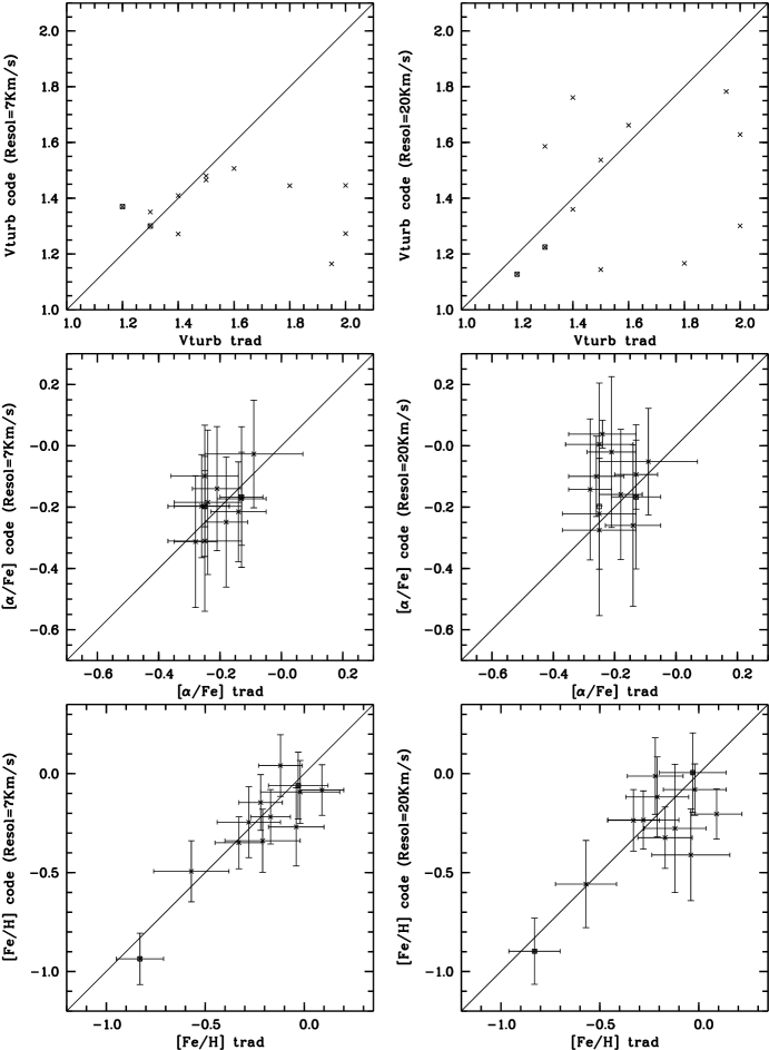
The results of this comparison is summarized in Table 3 and is plotted in Fig. 5. It may be seen that the metallicity and the $\alpha$ enhancement derived from our automatic procedure are consistent at $1\sigma$ with the results of a traditional analysis, when the dispersion of results of individual features is taken as error estimate. This in spite of the fact that in the traditional analysis in two cases the gravity has been changed to satisfy the iron ionization equilibrium, while no such thing is possible in the present version of our procedure. The mean metallicity difference in the sense (code – traditional) is $-0.04$ dex with a standard deviation of 0.11 dex. The mean difference in [$\alpha$/Fe] is +0.013 dex with a standard deviation of 0.074 dex. The mean difference in $\xi$ is $-0.21$ $\mathrm{kms}^{-1}$with a standard deviation of 0.32 $\mathrm{kms}^{-1}$. A possible cause of concern, looking at the top panel of Fig. 5, is that there appears to be no correlation between the $\xi$ measured by the code and the traditional abundance analysis. In fact what happens is that for eight of the stars there is a tight correlation, whereas for the remaining four there is no significant correlation, as can be inferred by computing Kendall’s $\tau$ for the two subsets. The reason for which $\xi$ is poorly determined in some cases is that, in general, there are few weak Fe i features. At low S/N ratios it may happen that most of them are rejected because the goodness-of-fit is too small. In these conditions $\xi$ is essentially undetermined. The comparison between automatic and traditional analysis suggests that the accuracy on $\xi$ is of the order of 0.3 $\rm kms^{-1}$, which implies an error in abundance of the order of 0.2 dex, for saturated lines. Since this is within the claimed accuracy of the method we believe it is not a serious problem. Furthermore we point out that several of the Ca i lines used for the determination of [$\alpha$/Fe] are saturated and the good agreement of these ratios between automatic and traditional analysis supports the above claim.

Table 3: Results of automatic and traditional analysis

Stara	S/N	$\rm T_{eff}$	gravity		[Fe/H]		[$\alpha$/Fe]		$\xi$ (km/s)
	@530nm		code	trad	code	trad	code	trad	code	trad
879b	17	4891.	2.50	2.50	$-0.25\pm 0.18$	$-0.28\pm 0.16$	$-0.17\pm 0.15$	$-0.13\pm 0.08$	1.3	1.4
772c	18	4891.	2.50	2.50	$-0.34\pm 0.16$	$-0.21\pm 0.19$	$-0.31\pm 0.23$	$-0.25\pm 0.12$	1.5	1.5
628	37	4904.	2.50	2.50	$-0.15\pm 0.14$	$-0.22\pm 0.11$	$-0.22\pm 0.16$	$-0.14\pm 0.09$	1.5	2.0
656	24	5017.	2.50	2.50	$-0.22\pm 0.14$	$-0.17\pm 0.10$	$-0.14\pm 0.20$	$-0.21\pm 0.08$	1.5	1.6
716	36	4967.	2.50	2.50	$+0.04\pm 0.16$	$-0.12\pm 0.11$	$-0.31\pm 0.21$	$-0.28\pm 0.07$	1.2	2.0
717	20	5042	2.50	2.50	$-0.08\pm 0.13$	$+0.09\pm 0.11$	$-0.25\pm 0.21$	$-0.18\pm 0.07$	1.3	1.3
894	34	4876.	2.50	2.50	$-0.27\pm 0.20$	$-0.04\pm 0.14$	$-0.10\pm 0.16$	$-0.25\pm 0.11$	1.4	1.4
432	28	4818.	2.50	2.30	$-0.94\pm 0.13$	$-0.83\pm 0.12$	$-0.17\pm 0.23$	$-0.13\pm 0.07$	1.3	1.3
635	19	4843.	2.50	2.50	$-0.35\pm 0.13$	$-0.33\pm 0.12$	$-0.20\pm 0.17$	$-0.26\pm 0.09$	1.4	1.8
867	20	4892.	2.50	2.50	$-0.49\pm 0.15$	$-0.57\pm 0.19$	$-0.03\pm 0.18$	$-0.09\pm 0.16$	1.3	2.0
927	43	4880.	2.50	2.75	$-0.06\pm 0.17$	$-0.03\pm 0.15$	$-0.20\pm 0.16$	$-0.25\pm 0.12$	1.4	1.2
709	41	4930.	2.50	2.50	$-0.09\pm 0.16$	$-0.02\pm 0.20$	$-0.18\pm 0.24$	$-0.24\pm 0.11$	1.5	1.5
a Star numbers are from Marconi et al. (1998) field 1, available through CDS
Starat cdsarc.u-strasbg.fr/pub/cats/J/A+A/330/453/sagit1.dat
b this is star [BHM2000] 139 of Bonifacio et al. (2000)
c this is star [BHM2000] 143 of Bonifacio et al. (2000)

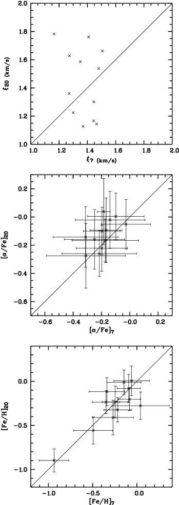
When degraded at a resolution R=15000 the mean difference in derived metallicity (in the sense UVES – [R=15000]) is +0.013 dex with a standard deviation of 0.15 dex. The mean difference in [$\alpha$/Fe] is –0.07 dex with a standard deviation of 0.08 dex. The mean difference in $\xi$ is –0.07 $\mathrm{kms}^{-1}$with a standard deviation of 0.29 $\mathrm{kms}^{-1}$. These comparisons are illustrated in Fig. 6. This shows that the resolution of 15000 is still sufficient to provide reliable abundances (see Fig.5). Since the actual resolution of Giraffe is higher it is even better suited to be used with our method.

5.2 Other elements

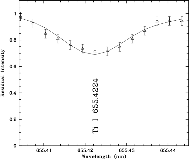
To check the behaviour of the code, we analyzed a few other elements for the two stars of Bonifacio et al. (2000) for which a complete abundance analysis is available. The results are reported in Table 4. For the other stars of the sample, the traditional abundance analysis is not yet complete. As can be seen from the table the results of traditional and automatic analysis are compatible within $1\sigma$ (being $\sigma$ the dispersion of individual features when more than one is available). In Fig.7 a fit for the Ti I 655.4224 nm line in star # 879 is plotted. Implementation of automatic analysis to obtain the abundances for several elements is our goal in the next future, the present results are encouraging.

Figure 7: Plot of the fit of a Ti i feature in star # 879. Solid line is the fit done by the code; the triangles are the experimental data pseudo-normalized; the bars are the errors of the observed spectrum.

Table 4: Results of automatic and traditional analysis for some elements

Element	code	$n$	traditional	$n$	code	$n$	traditional	$n$
	star #879				star #772
Ni i	$-0.64\pm 0.11$	6	$-0.56\pm 0.16$	6	$-0.44\pm 0.21$	6	$-0.63\pm 0.10$	6
Si i	$-0.26\pm 0.12$	4	$-0.35\pm 0.26$	5	$-0.28\pm 0.09$	5	$+0.06\pm 0.21$	4
Ti i	$-0.21\pm 0.05$	6	$-0.19\pm 0.13$	7	$-0.19\pm 0.13$	7	$-0.21\pm 0.05$	6
Ti ii	$-0.47\pm 0.13$	2	$-0.31\pm 0.07$	2	$-0.46\pm 0.06$	2	$-0.43\pm 0.18$	3
V i	$-0.15$	1	$-0.21\pm 0.16$	2	$-0.49$	1	$-0.44\pm 0.05$	2

6 Conclusions

We have built an automatic procedure to derive chemical abundances from high resolution spectra. The procedure is specifically targeted to the analysis of giants of the Sgr dSph, thus the grid of synthetic spectra and spectral features employed in the analysis are optimized for stars of spectral type and metallicity range appropriate to this case. Making use of Monte Carlo simulations we have shown that the procedure is quite stable and provides highly reproducible results. Comparison with the results obtained on 12 UVES spectra of Sgr dSph giants which have been independently analyzed in the traditional way by Bonifacio et al. (2000) and Bonifacio et al (2002) allows us to conclude that the automatic procedure provides results which are consistent at $1\sigma$ with the traditional analysis.

We plan to use the procedure described in this paper to obtain abundances for statistically significant numbers of Sgr giants as soon as data from the FLAMES facility are available. Our tests with UVES spectra degraded at the resolution of 15000 suggest that both spectrographs fed by OzPoz shall provide abundances of comparable accuracy, the lower resolution of Giraffe being to some extent compensated by the higher S/N achieved.

The reliability of our results is limited by the grid of synthetic spectra used to interpret the data. For example any error in the atomic or molecular data used in the computation will result in an error in the derived abundances. However whenever new and better grids of synthetic spectra are available it shall be straightforward to implement them in the procedure.

One weak point of our procedure is to assume that only the $\alpha$ elements have a direct effect on the temperature structure of the model. Another is to assume that all the $\alpha$ elements vary in lockstep and that their ratio to iron is fixed by the ratios of Mg and Ca. The validity of this latter hypothesis may be checked directly by looking at the abundances of Si and Ti. If non solar ratios of these elements to Mg and Ca are found the results of our procedure may be called into question.

The concept of our procedure may be generalized to the analysis of stars of different spectral type and/or luminosity class. In this case however it may not be enough to compute a new set of synthetic spectra, but also the spectral features and spectral ranges employed should be reconsidered based on the study of real and synthetic spectra.