The last stand before MAP: cosmological parameters from lensing, CMB and galaxy clustering

Abstract

Cosmic shear measurements have now improved to the point where they deserve to be treated on par with CMB and galaxy clustering data for cosmological parameter analysis, using the full measured aperture mass variance curve rather than a mere phenomenological parametrization thereof. We perform a detailed 9-parameter analysis of recent lensing (RCS), CMB (up to Archeops) and galaxy clustering (2dF) data, both separately and jointly. CMB and 2dF data are consistent with a simple flat adiabatic scale-invariant model with $\Omega_{\Lambda}=0.72\pm 0.09$, $h^{2}\Omega_{\rm cdm}=0.115\pm 0.013$, $h^{2}\Omega_{\rm b}=0.024\pm 0.003$, and a hint of reionization around $z\sim 8$. Lensing helps further tighten these constraints, but reveals tension regarding the power spectrum normalization: including the RCS survey results raises $\sigma_{8}$ significantly and forces other parameters to uncomfortable values. Indeed, $\sigma_{8}$ is emerging as the currently most controversial cosmological parameter, and we discuss possible resolutions of this $\sigma_{8}$ problem. We also comment on the disturbing fact that many recent analyses (including this one) obtain error bars smaller than the Fisher matrix bound. We produce a CMB power spectrum combining all existing experiments, and using it for a “MAP versus world” comparison next month will provide a powerful test of how realistic the error estimates have been in the cosmology community.

]

I Introduction

An avalanche of precision data has revolutionized our ability to constrain cosmological models and their free parameters in recent years [1, 2, 3, 4, 5, 6, 7, 8, 9, 10, 11, 12, 13, 14, 15, 16, 17, 18, 19, 20, 21, 22, 23, 24, 25, 26, 27, 28, 29, 30, 31, 32, 33, 34, 35, 36]. Around 1998, cosmic microwave background (CMB) data had become good enough to allow a realistic high-dimensional parameter space to be explored by fitting theoretical models directly to the measured CMB power spectrum (e.g., [8, 7]). In contrast, other cosmological constraints were included merely as priors on individual parameters, for instance the baryon density from Big Bang nucleosynthesis, the matter density from galaxy cluster abundance and the Hubble parameter from direct observations.

With the advent of improved galaxy redshift surveys like PSCz [37], 2dF [38] and SDSS [39], the galaxy power spectrum $P(k)$ was upgraded and admitted to the “CMB club”: it was so accurately measured that people started fitting models directly to the measured $P(k)$ curve rather than merely to some phenomenological parametrization thereof (say in terms of an amplitude and a “shape parameter”) [8, 9, 23]. The Lyman $\alpha$ forest (Ly$\alpha$F) power spectrum has now undergone the same upgrade [11, 30]

One promising cosmological probe is still conspicuously absent from this club and has so far been left out in the cold: the cosmic shear power spectrum measured with weak gravitational lensing. Like the CMB, it has the advantage of probing the dark matter distribution directly [40], without murky bias issues. Despite the spectacular progress since this elusive signal was first detected in 2000 [41, 42, 43, 44], increasing the sky area covered by almost two orders of magnitude [40, 45, 46, 47, 48, 49, 50, 51, 52], it has so far only been included in cosmological parameter studies as a prior on two parameters: the power spectrum normalization and the matter density. Yet it has been shown that the detailed shape of the weak lensing power spectrum $P_{\kappa}(\l)$ potentially contains almost as much cosmological information as the CMB [53, 54, 55], with great prospects for degeneracy breaking and cross-checking.

The goal of this paper is to treat weak lensing on an equal footing with CMB and galaxy clustering, fitting theoretical models directly to the CMB, LSS and lensing power spectra. Our results can also be viewed as the last stand before MAP: using our constraints combining the state-of-the-art available data for a “MAP versus world” comparison next month will provide a powerful test of how realistic the error estimates and underlying assumptions have been in the cosmology community.

The rest of this paper is organized as follows. We present our analysis method in Section II, describe the CMB, galaxy and lensing data used in Section III, compute quantitative model constraints in Section IV and discuss our conclusions in Section V.

II Method

In this section, we briefly describe our method for constraining cosmological models.

A General method

We use the grid-based multiparameter analysis method described in detail in [8, 9, 30], with modifications as described below. It involves the following steps:

1. Compute CMB and galaxy power spectra and the weak lensing aperture mass variance for a grid of models in our 9-dimensional parameter space.

2. Compute a likelihood for each model that quantifies how well it fits the data.

3. Perform 9-dimensional interpolation and marginalization to obtain constraints on individual parameters and parameter pairs.

As in [30], the we parametrize cosmology with the 11 parameters

$${\bf p}\equiv(\tau,\Omega_{\rm k},\Omega_{\Lambda},\omega_{\rm dm},\omega_{\rm b},f_{\nu},n_{s},n_{t},A_{s},r,b).$$ (1)

They are the reionization optical depth $\tau$, the primordial amplitudes $A_{s}$, $rA_{s}$ and tilts $n_{s}$, $n_{t}$ of scalar and tensor fluctuations, the bias parameter $b$ defined as the ratio between rms galaxy fluctuations and rms matter fluctuations on large scales, and five parameters specifying the cosmic matter budget, curvature $\Omega_{\rm k}$, vacuum energy $\Omega_{\Lambda}$, cold dark matter $\Omega_{\rm cdm}$, hot dark matter (neutrinos) $\Omega_{\nu}$ and baryons $\Omega_{\rm b}$. The quantities $\omega_{\rm b}\equiv h^{2}\Omega_{\rm b}$ and $\omega_{\rm dm}\equiv h^{2}\Omega_{\rm dm}$ correspond to the physical densities of baryons and total (cold + hot) dark matter ($\Omega_{\rm dm}\equiv\Omega_{\rm cdm}+\Omega_{\nu}$), and $f_{\nu}\equiv\Omega_{\nu}/\Omega_{\rm dm}$ is the fraction of the dark matter that is hot. We assume that the galaxy bias $b$ is constant on large scales [56]. We make $A_{s}$ as a discretized parameter to marginalize and find a best fit of $\sigma_{8}$ later in computation, as comparing to an undiscretized $A_{s}$ in previous papers[30]. Throughout this paper, we assume a negligible contribution from spatial curvature and massive neutrinos, setting $\Omega_{\rm k}=f_{\nu}=0$. Our final parameter grids are as follows:

• $\tau=0,0.05,0.1,0.2,0.3,0.5,0.8$

• $\Omega_{\Lambda}=0,0.1,....,1.0$

• $\omega_{\rm dm}=.02,.05,.08,.11,.13,.16,.20,.50$

• $\omega_{\rm b}=.003,.015,.018,.020,.022,.025,.03,.04,.07$

• $n_{s}=0.5,0.7,0.8,0.9,1.0,1.1,1.2,1.4,1.7$

• $n_{t}=-1.0,-0.7,-0.4,-0.2,-0.1,0$

• $r=0,0.1,0.2,0.3,0.4,0.6,0.8,1.0,1.4,1.8$

• $A_{s}=0.2,0.3,0.4,0.5,0.6,0.7,0.8,0.9$

• $b=0.5,0.6,0.7,0.8,0.9,1.0,1.1,1.2,1.3,1.4$

For each grid point in parameter space, we compute CMB and matter power spectra using the method detailed in [9]. We compute the corresponding theoretical lensing predictions as described in the following section. Although these lensing computations follow a fairly standard procedure, our procedure is described explicitly below to make clear which approximations we make.

B Lensing calculations

The lensing measurements that we will use are quoted in terms of the variance of the aperture mass $M_{\rm ap}$, given by[57, 58]:

$$\langle M_{\rm ap}^{2}(\theta)\rangle=2\pi\int^{\infty}_{0}\ell P_{\kappa}(\ell)\left[{12\over\pi(\ell\theta)^{2}}J_{4}(\ell\theta)\right]^{2}d\ell,$$ (2)

where $J_{4}$ is the fourth-order Bessel function of the first kind and $P_{\kappa}(\ell)$ is the convergence power spectrum, given by [57, 58, 59, 60]

$$P_{\kappa}(\ell)=\frac{9H_{0}^{4}\Omega_{\rm m}^{2}}{4c^{4}}\int_{0}^{w_{H}}{\overline{W}(w)^{2}\over a(w)^{2}}P^{nl}_{\delta}\left[{\ell\over f_{K}(w)},z(w)\right]dw.$$ (3)

Here $P^{nl}_{\delta}(k,z)$ is the nonlinear mass power spectrum, and $a(w)=[1+z(w)]^{-1}$ is the cosmic scale factor. $w$ is the radial comoving distance defined by

$$w(z)=\int_{0}^{z}{c\over H(z^{\prime})}dz^{\prime},$$ (4)

and $w_{H}\equiv w(\infty)$ is the comoving distance to the horizon. The time-variation of the Hubble parameter $H$ is given by

$${H\over H_{0}}=\sqrt{(1+z)^{3}\Omega_{\rm m}+(1+z)^{2}(1-\Omega_{\rm m}-\Omega_{\Lambda})+\Omega_{\Lambda}}.$$ (5)

$f_{K}(w)$ is the comoving angular diameter distance out to $w$, given by

$$f_{K}(w)=\left\{\begin{array}[]{lll}K^{-1/2}\sin(K^{-1/2}w)&\mbox{$K>0$}\\ w&\mbox{$K=0$}\\ (-K)^{-1/2}\sinh((-K)^{-1/2}w)&\mbox{$K<0$}\end{array}\right.$$ (6)

where $K$ is the spatial curvature defined by

$$K\equiv-\left({H_{0}\over c}\right)^{2}\Omega_{\rm k},\quad\Omega_{\rm k}\equiv(1-\Omega_{\rm m}-\Omega_{\Lambda}).$$ (7)

The weighting function $\overline{W}(w)$ is the source-averaged distance ratio

$$\overline{W}(w)=\int_{w}^{w_{H}}G(w^{\prime}){f_{K}(w^{\prime}-w)\over f_{K}(w^{\prime})}dw^{\prime},$$ (8)

where $G(w)=G(w(z))$ is the source redshift distance distribution, usually approximated by a fitting function of the form

$$G(w)={\beta\over z_{0}\Gamma({1+\alpha\over\beta})}\left({z\over z_{0}}\right)^{\alpha}e^{-(z/z_{0})^{\beta}},$$ (9)

with fitting parameters $z_{0}$,$\alpha$ and $\beta$.

The linear power spectrum at redshift $z$ is related to the present one by

$$P^{\rm linear}_{\delta}(z,k)=\left[{g(z)\over g(0)}\right]^{2}P^{\rm linear}_{\delta}(0,k),$$ (10)

where the linear growth factor $g(z)$ is approximately given by [61]

$$g(z)\approx{5\over 2}\Omega_{\rm m}^{z}\left[{\Omega_{\rm m}^{z}}^{4/7}-\Omega_{\Lambda}^{z}+\left(1+{\Omega_{\rm m}^{z}\over 2}\right)\left(1+{\Omega_{\Lambda}^{z}\over 70}\right)\right]^{-1}.$$ (11)

Here the parameters $\Omega_{\rm m}^{z}$ and $\Omega_{\Lambda}^{z}$ are those at redshift $z$, given by the present values $\Omega_{\rm m}$ and $\Omega_{\Lambda}$ through the relations

$$\Omega_{\rm m}^{z}=\left[{H_{0}\over H(z)}\right]^{2}\Omega_{\rm m}(1+z)^{3},$$ (12)

$$\Omega_{\Lambda}^{z}=\left[{H_{0}\over H(z)}\right]^{2}\Omega_{\Lambda},$$ (13)

with $H(z)$ given by equation (5).

The power spectrum $P^{nl}_{\delta}(k)$ needed in equation (3) is the nonlinear one rather than the linear one $P^{l}_{\delta}(k)$ given by equation (10). Based on a pioneering idea of Hamilton et al. [62], a series of approximations [59, 63, 64, 65] have been developed for approximating the former using the latter. In terms of the dimensionless power

$$\Delta^{2}(k)\equiv{4\pi\over(2\pi)^{3}}k^{3}P_{\delta}(k),$$ (14)

the linear power $\Delta_{\rm l}$ on scale $k_{\rm l}$ is approximately related to the nonlinear power $\Delta_{\rm nl}$ on a smaller nonlinear scale $k_{\rm nl}$. We use the Peacock & Dodds’ approximation [65], where this mapping is given by

$$\Delta_{nl}^{2}(k_{nl})=f_{nl}\left[\Delta_{l}^{2}(k_{l})\right]$$ (15)

and

$$k_{l}=\left[1+\Delta_{nl}^{2}(k_{nl})\right]^{-1/3}k_{nl},$$ (16)

with a fitting function

$$f_{nl}(x)=x\left\{{1+B\beta x+(Ax)^{\alpha\beta}\over 1+\left[{(Ax)^{\alpha}g(0)^{3}\over(Vx^{1/2})}\right]^{\beta}}\right\}^{1/\beta},$$ (17)

parametrized by

$$A = 0.482(1+n_{\rm eff}/3)^{-0.947},$$ (18)

$$B = 0.226(1+n_{\rm eff}/3)^{-1.778},$$ (19)

$$\alpha = 3.310(1+n_{\rm eff}/3)^{-0.224},$$ (20)

$$\beta = 0.862(1+n_{\rm eff}/3)^{-0.287},$$ (21)

$$V = 11.55(1+n_{\rm eff}/3)^{-0.423}.$$ (22)

Here $g(0)$ is the linear growth factor of equation (11) evaluated at $z=0$ and $n_{\rm eff}\equiv d\ln P_{\delta}^{\rm l}(k)/d\ln k_{\rm l}$ is the effective logarithmic slope of the linear power spectrum evaluated at $k_{\rm l}$. Since this slope should be evaluated for a model without baryonic wiggles, we compute $n_{\rm eff}$ using an the Eisenstein & Hu fitting function with baryon oscillations turned off.

III Experimental data used

A CMB data

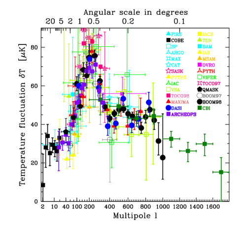
Figure 1 shows the 135 CMB measurements which are used in our analysis. Compared to the data set we used in [30], we add the new measurements from the Cosmic Background Imager (CBI) mosaic[66], the Very Small Array (VSA) [67] and Archeops [68]. For CBI, we use the year 2000 observations of three pairs of mosaic fields [66] but not the deep fields, because it is still unclear whether their signal is dominated by CMB or other effects such as SZ effect[69]. The Boomerang results updated last week [70] and the Acbar results [71] became available too recently for inclusion in this analysis, but we do include them in the online combined power spectrum described below.

FIG. 1.: CMB data used in our analysis. Error bars do not include calibration or beam errors which allow substantial vertical shifting and tilting for some experiments (these effects are included in our analysis).

We combine these measurements into a single set of 28 band powers shown in Figure 2 and Table 1 using the method of [30] as improved in [31], including calibration and beam uncertainties, which effectively calibrates the experiments against each other. Since our compressed band powers $d_{\l}$ are simply linear combinations of the original measurements, they can be analyzed ignoring the details of how they were constructed, being completely characterized by a window matrix ${\bf W}$:

$$\langle d_{i}\rangle=\sum_{\l}{\bf W}_{i\l}\delta T_{\l}^{2},$$ (23)

where $\delta T_{\l}^{2}\equiv\l(\l+1)C_{\l}/2\pi$ is the angular power spectrum. This matrix is available at $www.hep.upenn.edu/{\sim}max/cmb/cmblsslens.html$ together with the 28 band powers $d_{\l}$ and their $28\times 28$ covariance matrix. The data $\l$-values and effective $\l$-ranges in Figure 2 and Table 1 correspond to the median, 20th and 80th percentile of the window functions ${\bf W}$. Comparing Table 1 with the older results from [31], we find that the only major change is a shallower rise towards the 1st peak due to Archeops, which is able to help calibrate Boomerang and other small-scale experiments by connecting them with the COBE. Specifically, $\delta T_{\l}$ has increased by about 10% at $\l\sim 50$ and decreased about 5% for $\l\sim 100-200$, thereby nudging the first peak a tad to the right.

FIG. 2.: Combination of data from Figure 1. These error bars include the effects of beam and calibration uncertainties, which cause long-range correlations of order 10% over the peaks. In addition, points tend to be anti-correlated with their nearest neighbors, typically at the level of 10-20%. The curve shows our model best fitting CMB+LSS data (second last column in Table 2).

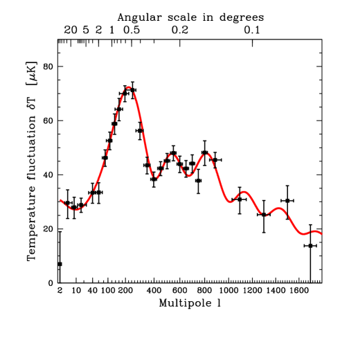
Table 1 – Band powers combining the information from CMB data from Figure 1. The 1st column gives the $\l$-bins used when combining the data, and can be ignored when interpreting the results. The 2nd column gives the medians and characteristic widths of the window functions as detailed in the text. The error bars in the 3rd column include the effects of calibration and beam uncertainty. The full $28\times 28$ correlation matrix and $28\times 2000$ window matrix are available at $www.hep.upenn.edu/\sim max/cmb/cmblsslens.html$.

$\l$-Band	$\l$-window	$\delta T^{2}\>[\mu$K${}^{2}]$
$2-2$	$2_{-0}^{+0}$	$49\pm 310$
$3-5$	$4_{-1}^{+3}$	$877\pm 308$
$6-10$	$8_{-2}^{+3}$	$782\pm 218$
$11-30$	$16_{-4}^{+9}$	$832\pm 151$
$31-50$	$40_{-10}^{+10}$	$1113\pm 244$
$51-75$	$60_{-13}^{+14}$	$1120\pm 255$
$76-100$	$87_{-12}^{+10}$	$2139\pm 279$
$101-125$	$110_{-17}^{+11}$	$2767\pm 340$
$126-150$	$135_{-14}^{+12}$	$3461\pm 443$
$151-175$	$161_{-23}^{+21}$	$4122\pm 529$
$176-225$	$196_{-34}^{+24}$	$4900\pm 410$
$226-275$	$246_{-44}^{+23}$	$5079\pm 441$
$276-325$	$297_{-28}^{+24}$	$3164\pm 359$
$326-375$	$348_{-23}^{+22}$	$1892\pm 265$
$376-425$	$398_{-22}^{+20}$	$1468\pm 213$
$426-475$	$450_{-22}^{+21}$	$1793\pm 219$
$476-525$	$499_{-22}^{+21}$	$2037\pm 257$
$526-575$	$549_{-23}^{+21}$	$2306\pm 268$
$576-625$	$600_{-22}^{+21}$	$1932\pm 267$
$626-675$	$649_{-22}^{+21}$	$1790\pm 259$
$676-725$	$700_{-21}^{+20}$	$1948\pm 293$
$726-775$	$749_{-23}^{+22}$	$1428\pm 334$
$776-825$	$801_{-23}^{+23}$	$2322\pm 438$
$826-1000$	$888_{-46}^{+52}$	$2067\pm 261$
$1001-1200$	$1093_{-65}^{+56}$	$953\pm 300$
$1201-1400$	$1299_{-55}^{+54}$	$638\pm 291$
$1401-1600$	$1501_{-55}^{+54}$	$924\pm 368$
$1601-\infty$	$1700_{-53}^{+51}$	$189\pm 273$

B LSS data

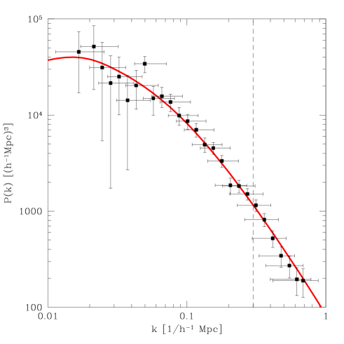
Measurements of $P(k)$ from Galaxy redshift surveys have recently improved in both quality and quantity, and the Sloan Digital Sky Survey is set to continue this trend. In this paper, we use the power spectrum from the 2dFGRS[72] as measured by [73]. We model the galaxy bias as a scale-independent constant $b$, and therefore discard all 2dF measurements with $k\geq 0.3h/$Mpc to minimize our sensitivity to nonlinear clustering and nonlinear bias effects.

FIG. 3.: 2dF galaxy power spectrum data used. We include only points leftward of the dotted line (with $k<0.3h/Mpc$) in our analysis to stay in the linear regime. The curve shows our model best fitting CMB+LSS data (second last column in Table 2).

C Lensing data

For this paper, we use the results from Hoekstra et al.[49], the analysis of 53 square degrees of $R_{C}$-band imaging data from the Red Sequence Cluster Survey(RCS). The RCS[45, 46] is a 100 square degree galaxy cluster optical survey designed to provide a large sample of optically selected clusters of galaxies with redshifts $0.1<z<1.4$ We use only the seven data points which have been used in cosmological analysis in[49]. We model the source redshift distribution, we use the multi-redshift part in equation (9), with $\alpha=4.7$, $\beta=1.7$ and $z_{0}=0.302$, which are the best fit value given by Hoekstra et al.[49].

FIG. 4.: Lensing data used in our analysis. The two curves show our best fit model excluding (bottom) and including (top) lensing data.

IV Parameter constraints

Our cosmological parameter constraints are summarized in Table 2. We study three cases: using CMB data only, adding LSS information and adding lensing measurements too, respectively. These three cases correspond to the three columns of the table and are discussed in the corresponding three subsections below.

A From CMB data alone

FIG. 5.: Constraints on individual parameters using only CMB information. The quoted $1-\sigma$ and $2-\sigma$ confidence limits are where each curve drops below the horizontal dashed lines $e^{-1^{2}/2}\approx 0.61$ and $e^{-2^{2}/2}\approx 0.14$, respectively.

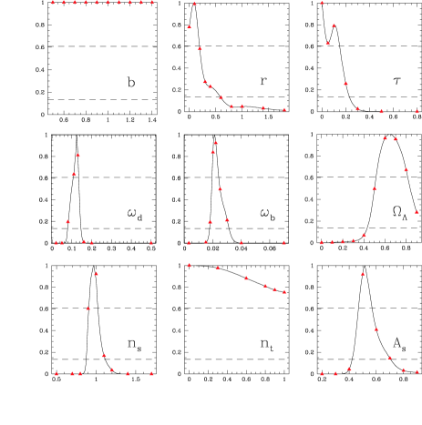
Figure 5 shows our constraints on nine individual cosmological parameters, using only the CMB data. Comparing to numerous previous analyses using CMB data alone [8, 9, 23, 30], we see that the addition of new CMB data from CBI, Archeops etc. has substantially tightened the constraints, especially on the tensor-to-scalar ratio $r$ and dark energy $\Omega_{\Lambda}$. CMB alone is seen to firmly rules out models with no dark matter and models with no dark energy. (The dark energy constraint depends critically on our prior assumption $\Omega_{\rm k}=0$, whereas the dark matter result does not.)

The last four constraints in Table 2 are computed with the moments method as in [30]. They are for parameters ($h$, $\beta$, $z_{\rm ion}$ and $\sigma_{8}$) that are not independent and merely functions of the 11 parameters that define our model grid. The Hubble parameter $h$ is given by

$$h=\sqrt{\omega_{\rm dm}+\omega_{\rm b}\over 1-\Omega_{\rm k}-\Omega_{\Lambda}}.$$ (24)

The redshift-space distortion parameter $\beta$ is given by [74, 75, 76]

$$\beta={f(\Omega_{\rm m},\Omega_{\Lambda})\over b},$$ (25)

where $f(\Omega_{\rm m},\Omega_{\Lambda})\approx\Omega_{\rm m}^{\rm 0.6}$ is the velocity-suppression factor[75, 76] (we evaluate $f$ exactly using the grow$\lambda$ package [74]). If the diffuse intergalactic hydrogen was reionized abruptly at a redshift $z_{\rm ion}$, then [77].

$$z_{\rm ion}\approx 8.9\left({{\tau h}\over\omega_{\rm b}}\right)^{2/3}\Omega_{\rm m}^{1/3}.$$ (26)

in the approximation that $z_{\rm ion}\gg 1$ (which we know to be the case). The alternative normalization parameter $\sigma_{8}$ is the rms fluctuation in an $8h^{-1}$ sphere, given by a weighted integral of the matter power spectrum [75].

Table 2 – Best fit values and $1-\sigma$ confidence limits on cosmological parameters. For the numbers above the horizontal line, the central values are the ones maximizing the likelihood (the best fit model). For the numbers below the horizontal line, the central values are means rather than those for the best fit model[30]. For instance, the Hubble parameters for the best fit models are $h=0.68$, $0.69$ and $0.61$ for the three columns, respectively, which differs from the mean values in the table.

	CMB alone	$+$ 2dF	$+$ RCS lensing
$\tau$	$0.04^{+.06}$	$0.06^{+.03}_{-.03}$	$0.20^{+.03}_{-.03}$
$\Omega_{\Lambda}$	$0.71^{+.11}_{-.11}$	$0.72^{+.09}_{-.09}$	$0.59^{+.08}_{-.08}$
$h^{2}\Omega_{\rm dm}$	$0.112^{+.014}_{-.014}$	$0.115^{+.013}_{-.013}$	$0.128^{+.008}_{-.008}$
$h^{2}\Omega_{\rm b}$	$0.023^{+.003}_{-.003}$	$0.024^{+.003}_{-.003}$	$0.024^{+.002}_{-.002}$
$n_{s}$	$0.99^{+.06}_{-.06}$	$0.99^{+.04}_{-.04}$	$1.00^{+.02}_{-.02}$
$As$	$0.54^{+.07}_{-.07}$	$0.55^{+.06}_{-.06}$	$0.78^{+.05}_{-.05}$
$r$	$0.10^{+.17}$	$0.08^{+.11}$	$0.02^{+.05}$
$b$		$0.87^{+.06}_{-.06}$	$0.89^{+.04}_{-.04}$
$h$	$0.71^{+.13}_{-.13}$	$0.73^{+.11}_{-.11}$	$0.61^{+.04}_{-.04}$
$\beta$	$0.40^{+.16}_{-.16}$	$0.39^{+.07}_{-.07}$	$0.46^{+.04}_{-.04}$
$z_{\rm ion}$	$4.82^{+5,97}$	$8.06^{+2.04}_{-2.04}$	$19.23^{+2.45}_{-2.45}$
$\sigma_{8}$	$0.72^{+.06}_{-.06}$	$0.74^{+.06}_{-.06}$	$0.92^{+.04}_{-.04}$
$\chi^{2}/n$	$23.7/21$	$38.7/40$	$61.2/47$

B From CMB+LSS data

FIG. 6.: Same as previous figure but combining CMB and LSS information.

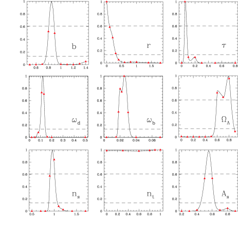
Figure 6 shows how the above-mentioned constraints tighten up when including the 2dF galaxy clustering data. The improvement comes mainly from breaking degeneracies involving curvature, dark energy, dark matter, baryons and tilt. The $\Omega_{\Lambda}$-measurement is seen to be nicely consistent with the many other pieces of evidence (SN Ia etc.) pointing towards $\Omega_{\rm m}\approx 0.7)$. The 2dF bias value $b\approx 0.87\pm 0.06$ (interpreted as the real-space bias at the effective survey redshift) is consistent with that found by the 2dF team [78, 79], although on the low side (since we are marginalizing over $b$, this has no impact on our constraints on other parameters such as $\sigma_{8}$). The most striking improvement is seen to be for the reionization optical depth $\tau$, hinting at a detection of reionization around $z\approx 8$. However, as we will discuss at length in Section V, the true significance of this detection is probably lower than Figure 6 suggests.

C From CMB, LSS and lensing data

1 One-Dimensional Constraints

FIG. 7.: Same as previous figure but combining CMB, LSS and lensing information.

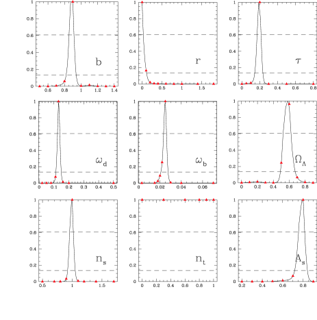
Above we saw that adding 2dF data to the CMB not only tightened parameter constraints, but also produced a consistent picture that agreed well with other measurements supporting the cosmological concordance model. Figure 7 shows that things are quite different when adding the RCS lensing data. Although the nominal constraints do get substantially sharper as predicted [54], most strikingly for the tensor-to-scalar ratio $r$, the harmonious consistency becomes clouded. Adding the 7 lensing data points raises $\chi^{2}$ by $22.5$ (from 38.7 to 61.2 for about 54 effective degrees of freedom). Although this per se might be considered acceptable, it is striking how much the lensing shifts the best-fit values of many parameters. Most notably, the reionization optical depth $\tau$ increases from $0.06\pm 0.03$ to $0.20\pm 0.03$ and the best fit cosmological constant $\Omega_{\Lambda}$ drops from $0.71$ to $0.55$, which sits uncomfortably with, e.g., SN Ia constraints. The cosmological model is pushed into an uncomfortably configuration by the lensing data, creaking and squeaking but refusing to outright collapse.

As we will see in Section V, this tension comes from the overall normalization of the power spectrum, with the RCS lensing data pushing the best-fit $\sigma_{8}$ value up from $0.71$ to $0.91$. This normalization agrees with that of some other cosmic shear surveys [47, 49, 50, 51], but not with that preferred by CMB and LSS data. In Section V, we will comment on uncertainties and other lensing data with different normalization.

2 Two-Dimensional Constraints

For more detailed insight into our parameter constraints and degeneracies, we now turn to joint constraints on pairs of parameters.

FIG. 8.: Constraints in the $(\tau,r)$-plane. The large pink/light grey region is ruled out by CMB alone at the 95% confidence level. The red/grey area shows the region excluded by adding additional constraints from 2dF. The black curve shows the allowed region when combine CMB, 2dF and RCS lensing.

FIG. 9.: Constraints in the $(n_{s},r)$ plane. The large pink/light grey region is ruled out by CMB alone. The red/grey region becomes ruled out when adding 2dF information. The black curve shows the allowed region when combine CMB, 2dF and RCS lensing.

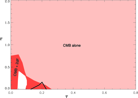
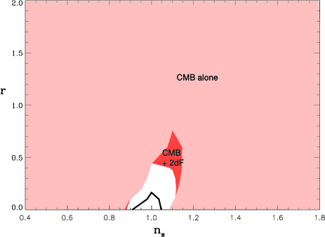
Figure 8 shows that 2dF breaks the CMB degeneracy between reionization and gravity waves and produces essentially independent (separable) constraints on $\tau$ and $r$. The gravity wave limits agree well with those found by [36] who also included 2dF and Archeops data. The fact that the allowed regions excluding and including lensing data have essentially no overlap illustrates the poor consistency between CMB+LSS and lensing data sets mentioned above.

Figure 9 shows constraints in the parameter space $(n_{s},r)$ where inflationary models can be tested. These limits from CMB only and from CMB+LSS are comparable with those in older work requiring stronger priors. For instance, comparison with a corresponding plot from a year ago [30] shows new data has squeezed the constraints substantially, particularly on the gravity wave amplitude. Now CMB data alone gives $r<0.48$ at 95% level, obtainable only be combining CMB and LSS data back then. Now CMB+2dF lowers the limit to $r<0.34$. The lensing data nominally helps even helps more, tightening the constraint to $r<0.13$ — we return to the issue of whether this is believable in Section V.

FIG. 10.: Constraints in the $(\omega_{\rm dm},\omega_{\rm b})$-plane. The large pink/grey region is ruled out by CMB data alone at 95% confidence. The smaller red/shaded region becomes excluded when imposing additional constraints from 2dF. The thick black curve shows the allowed region when combine CMB, 2dF and RCS. The rectangular band by the thin straight lines shows the BBN constraints from [87].

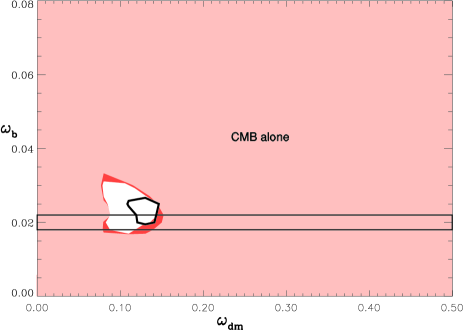
Let us now turn to the cosmic matter budget. A year ago [30, 23], the CMB+LSS constraints on the baryon density $\omega_{\rm b}$ were beautifully consistent with those from Big Bang Nucleosynthesis (BBN), $\omega_{\rm b}=0.02\pm 0.002$. Although the agreement is still acceptable, Figure 10 shows that the CMB+LSS baryon density is creeping back up again towards the higher range that was favored two years ago [1, 2]. This slight tension is reflected in $\chi^{2}$ increasing by 3 if we add a the BBN prior to our likelihood analysis.

V Discussion

Since cosmic shear measurements have now improved to the point where they deserve to be treated on par with CMB and galaxy clustering data, we have perform a detailed 9-parameter analysis of recent lensing, CMB and galaxy clustering data.

For the CMB part, we constructed and used a data set combining all available data taking calibration errors and beam uncertainties into account, effectively calibrating them off of each other. Using this combined power spectrum for a “MAP versus world” comparison next month will provide a powerful test of how realistic the error estimates have been in the CMB community.

Even though 2002 has added substantial amounts of information on the CMB power spectrum, e.g., from CBI and Archeops, the combined CMB and 2dF data remains comfortably consistent with a simple flat adiabatic scale-invariant concordance model with $\Omega_{\Lambda}=0.72\pm 0.09$, $h^{2}\Omega_{\rm cdm}=0.115\pm 0.013$ and $h^{2}\Omega_{\rm b}=0.024\pm 0.003$. The new data has added a hint of reionization around $z\sim 8$. These constraints assumed negligible contributions from spatial curvature and massive neutrinos.

Including the RCS lensing data in our analysis confirmed with real data what was predicted by Fisher matrix forecasts [54]: that lensing has the statistical power to substantially help with cosmological parameter constraints in two ways: by breaking degeneracies and by providing cross-checks. Intriguingly, one of the cross-checks failed, so let us now turn to this failure in more detail.

A The $\sigma_{8}$ problem

Our results suggest that the tension between the lensing and other data comes from the overall normalization of the power spectrum. We saw that the CMB+2dF data preferred $\sigma_{8}=0.74$, in good agreement with results from last year [78]. In contrast, the RCS lensing data prefers higher values [49] and pushed the normalization up to $\sigma_{8}=0.92$ in our joint analysis.

Physically, it is easy to see why this pushed other parameters in the way it did, notably increasing $\tau$ and decreasing $\Omega_{\Lambda}$. If we increase the value of $\sigma_{8}$, the CMB and galaxy power spectra will both increase in amplitude. This causes no problems for fitting the 2dF data, since our method can merely readjust their bias, but causes serious difficulties with the CMB. The acoustic peaks can be brought back down to acceptable heights by increasing $\tau$, but this provides only a partial solution to the problem, since it leaves the power on very large $\l\mathrel{\hbox to0.0pt{\lower 3.0pt\hbox{$\mathchar 536\relax$}\hss}\raise 2.0pt\hbox{$\mathchar 316\relax$}}10$ scales larger than observed by COBE DMR. Lowering $\Omega_{\Lambda}$ helps with this, since it increases the linear growth factor and thereby lowers the entire CMB power spectrum for fixed current matter clustering. $\Omega_{\Lambda}$ can only be lowered by a moderate amount, however, since the matter density $\Omega_{\rm m}\sim 1-\Omega_{\Lambda}$ will increase and give the galaxy power spectrum the wrong shape. The response of the parameter fitting algorithm is therefore to do a little bit of both tweaks, increasing $\tau$ and lowering $\Omega_{\Lambda}$. Indeed, similar results were obtained in a smalled parameter space by Hoekstra et al. [49], who found that they could only reconcile their lensing normalization with CMB for a rather large reionization optical depth $\tau=0.12\pm 0.04$.

To verify that this is the correct physical interpretation of what is going on, we repeated our entire analysis with the amplitude of the RCS data lowered by a factor of $(0.7/0.86)^{2}$, which is roughly the ratio of normalizations preferred by CMB+2dF and RCS respectively. This analysis gave results fully consistent with those from CMB+2dF alone, for example, $\tau=0.05\pm 0.03$, $\Omega_{\Lambda}=0.76\pm 0.13$, $\omega_{\rm dm}=0.11\pm 0.02$, $\omega_{\rm b}=0.024\pm 0.005$, $n_{s}=1.00\pm 0.04$, $A_{s}=0.52\pm 0.10$, $r=0.10+0.23$, $b=0.82\pm 0.09$, $z_{ion}=7.64\pm 3.18$ and $\sigma_{8}=0.70\pm 0.11$. These results not only demonstrate consistency, but also show that by combining lensing and CMB and LSS, we can get stronger constraints on parameters like $\Omega_{\Lambda}$, $n_{s}$, $\sigma_{8}$ and $z_{ion}$, just as had been predicted using information theory [54].

Table 3 – Recent measurements of the power spectrum normalization $\sigma_{8}$. For results quoted as fitting formulas involving $\Omega_{\rm m}$, we have set $\Omega_{\rm m}=0.3$. Error bars are $1\sigma$ — for [49] and [52], we have simply divided their quoted 95% errors by 2.

Analysis		$\sigma_{8}$
Clusters:
Pierpaoli et al. (2001)	[88]	$1.02^{+0.07}_{-0.08}$
Borgani et al. (2001)	[89]	$0.76^{+0.08}_{-0.05}$
Reiprich & Böhringer (2001)	[90]	$0.68^{+0.08}_{-0.06}$
Seljak et al. (2001)	[91]	$0.75\pm 0.06$
Viana et al. (2001)	[92]	$0.61\pm 0.05$
Bahcall et al. (2002)	[93]	$0.72\pm 0.06$
Pierpaoli et al. (2002)	[94]	$0.77^{+0.05}_{-0.04}$
Weak lensing:
Jarvis et al. (2002)	[52]	$0.71^{+0.06}_{-0.08}$
Brown et al. (2002)	[95]	$0.74\pm 0.09$
Hoekstra et al. (2002)	[49]	$0.86^{+0.04}_{-0.05}$
Van Waerbekeet al. (2002)	[51]	$0.97\pm 0.06$
Baconet al. (2002)	[47]	$0.97\pm 0.13$
Refregieret al. (2002)	[50]	$0.94\pm 0.14$
CMB:
Lahav et al. 2001	[78]	$0.73\pm 0.05$
Melchiorri & Silk 2002	[34]	$0.70\pm 0.05$
Lewis et al. 2002	[32]	$0.79\pm 0.06$
This work		$0.74\pm 0.06$

So is the CMB normalization too low or is the lensing normalization too high? As shown in Table 3, $\sigma_{8}$ is emerging as the currently most controversial cosmological parameter, and it will be crucial to use further cosmological data to get to the bottom of this issue. The table illustrates what has been emphasized by many authors, namely that the scatter between $\sigma_{8}$ measurements using different techniques is substantially larger than the formal error bars, triggering unpleasant flashbacks to the bimodal and bitter debate about the Hubble parameter $h$. Although much work clearly needs to be done to resolve this issue, there are some encouraging indications that the $\sigma_{8}$ gap may be closing. The CMB normalization has increased slightly in the last year, with the first acoustic peak growing by $10\%$ between [30] and our present compilation. CMB experiments can now be more effectively calibrated off of each other, and Archeops connects the calibration of DMR to that of the many experiments sensitive to the 1st acoustic peak and beyond. The cluster normalization has dropped somewhat because of recalibrations of the mass-temperature relation (see Table 3).

Although the lensing normalization has been uniformly high across groups [47, 49, 50, 51], the largest and most recent data set released has now produced the much lower normalization $\sigma_{8}\approx 0.71$ [52] (for $\Omega_{\rm m}=0.3$). Indeed, the Hoekstra et al. normalization may also be coming down by 5-10% (Hoekstra, private communication), partly because of a new and more accurate version of the Peacock & Dodds fitting formula [65].

Moreover, our analysis did not marginalize over the source redshift parameters $\alpha=4.7$, $\beta=1.7$ and $z_{0}=0.302$ from equation (9), but merely used the best fit values from [49]. Such marginalization would be expected to somewhat weaken the $\sigma_{8}$ constraints that we obtained from the RCS lensing data. As an extreme example, we recomputed the shear power spectrum $P_{\kappa}(\l)$ replacing the characteristic source redshift parameter $z_{s}=0.302$ with the $3-\sigma$ lower and upped limits on its value from [49]. These extreme values $z_{s}=z=0.274$ and $z_{s}=0.337$ made the shear fluctuation amplitude $10-15\%$ lower and higher, respectively, so lowering the source redshifts at the $2\sigma$ level would close approximately half of the $\sigma_{8}$ gap between the RCS and the CMB. Despite the current discord, there is thus real hope that a beautiful consistent picture of cosmology will eventually emerge.

B Are the constraints too good to be true?

In addition to the above-mentioned tension regarding the best fit values of some parameters, there is a slight puzzle regarding their error bars: some constraints seem a bit too good to be true. Specifically, the CMB error bars in Table 2 are in some cases comparable to those forecast for MAP [96] using the Fisher matrix technique [97]. This puzzling fact is not limited to the present paper, but appears rather generic. For instance, consider the scalar spectral index $n_{s}$. The forecast for MAP (2 years of data including polarization) is accuracy $\Delta n_{s}=0.11$ with no prior assumptions, $\Delta n_{s}=0.045$ assuming $\Omega_{\rm k}=0$ and $\Delta n_{s}=0.021$ when adding SDSS galaxy clusterinng data (the final luminous red galaxy sample) [96]. We found $\Delta n_{s}=0.06$ from current CMB alone (Table 2, assuming $\Omega_{\rm k}=0$), comparable to other studies in the recent literature. For instance, Lewis & Bridle [32] obtain $\Delta n_{s}=0.04$ including 2dF data, and the Boomerang team reports $\Delta n_{s}=0.06-0.08$ for various priors [70].

To gain insight into this puzzle, we compute the Fisher matrix [97] corresponding to the current data. In the approximation that all the CMB information is coming from the mean rather than the covariance of the power, the equations in [97] give

$${\bf F}_{\rm cmb}={\bf D}^{t}{\bf W}\SS^{-1}{\bf W}^{t}{\bf D},$$ (30)

where $\SS$ is the $28\times 28$ covariance matrix of our combined CMB power spectrum measurements from Section III A, ${\bf W}$ is the corresponding $\l_{\rm max}\times 28$ window matrix and the $\l_{\rm max}\times 28$ matrix

$${\bf D}_{\l i}\equiv{\partial\over\partial p_{i}}\delta T_{\l}^{2}$$ (31)

gives the derivatives of the power spectrum with respect to the cosmological parameters $p_{i}$. We compute an analogous Fisher matrix ${\bf F}_{\rm 2df}$ using the covariance matrix and window functions for the 2dF power spectrum from [73]. We then evaluate the attainable error bars from CMB alone as $\Delta p_{i}=({\bf F}_{\rm cmb}^{-1})_{ii}^{1/2}$ and from CMB+2dF as $\Delta p_{i}=([{\bf F}_{\rm cmb}+{\bf F}_{\rm 2df}]^{-1})_{ii}^{1/2}$. For the scalar spectral index with an $\Omega_{\rm k}=0$ prior, this gives $\Delta n_{s}=0.16$ from CMB alone and $\Delta n_{s}=0.13$ for from CMB+2dF, a factor 2-3 larger than the above-mentioned likelihood analysis results from us and others.

Comparing with our Fisher matrix results, the most suspicious error bar in Table 2 is that on the optical depth $\tau$, where we quoted $\Delta\tau=0.06$ from CMB alone and the Fisher matrix gives $\Delta\tau=0.18$. For the $\tau$ case, there is wide scatter in the literature. On the optimistic side, the CBI team reported $\tau=0.09^{+.14}_{-0.07}$[29], and a strong detection of reionization was claimed from earlier data [98]. On the pessimistic side, the 2dF and Boomerang teams report a $2\sigma$ limit $\tau<0.5$ [23, 70], in line with the Fisher forecast.

If our $\tau$ errors are indeed too small due to some artifact of our method, this would weaken the constraints on the normalization $\sigma_{8}$, since CMB constrains mainly the combination $\sigma_{8}e^{-\tau}$. However, the conclusion that $\sigma_{8}=0.9$ forces the uncomfortably high value $\tau\approx 0.2$ would still stand, since it follows directly from this scaling relation.

Efstathiou & Bond [99] have shown that there are physically understandable reasons why the Fisher matrix approach can significantly overestimate the errors on cosmological parameters, especially when strong degeneracies are present and that the curvature of a banana-shaped allowed region becomes important. This is indeed the case with $\tau$, with its strong degeneracy with the normalization parameter $A_{s}$, and a rigorous Bayesean confidence interval taking into account the asymmetry $\tau\geq 0$ (neglected in the Fisher treatment) also matters. “Weak” priors can also have a strong effect, notably on $h$ and gravity waves. Hopefully, our concerns will therefore go away when the MAP data arrives, in particular when all major degeneracies are broken with other datasets and priors. Since equation (30) is trivial to apply, it would be prudent to include a Fisher analysis of the data used in all future parameter constraint papers, as a reality check.

C Outlook

In conclusion, the pace at which new measurements have tightened up constraints on cosmological parameters is breathtaking. The constraints become particularly tight if one uses theoretical prejudice to impose spatial flatless $\Omega_{\rm k}=0$ like we have done, interpreting the CMB indication $\Omega_{\rm k}\approx 0$ as support for inflation and perfect flatness and thereby breaking the worst parameter degeneracy of all by fiat. It can be argued that precision cosmology is already here, before MAP, and now faces its first baptism of fire: will the current precision measurements of cosmological parameters agree with MAP? Next month we will know whether the whole edifice goes down in flames or stands stronger than ever.

The authors wish to thank Gary Bernstein, Karim Benabed and Roman Scoccimarro for helpful comments. This work was supported by NSF grants AST-0071213, AST-0134999, AST-0098606 and PHY-0116590, NASA grants NAG5-9194, NAG5-11099, NAG5-10923 and NAG5-10924 and a Keck foundation grant. MT and MZ are David and Lucile Packard Foundation Fellows MT is a Cottrell Scholar of Research Corporation.

REFERENCES

- [1] A. E. Lange et al., Phys. Rev. D 63, 042001 (2001).
- [2] M. Tegmark and M. Zaldarriaga, Phys. Rev. Lett. 85, 2240 (2000).
- [3] A. Balbi et al., ApJL 545, L1 (2000).
- [4] W. Hu, M. Fukugita, M. Zaldarriaga, and M. Tegmark, ApJ 549, 669 (2001).
- [5] A. Jaffe et al., Phys. Rev. Lett. 86, 3475 (2000).
- [6] T. Padmanabhan and S. K. Sethi, ApJ 555, 125 (2001).
- [7] C. H. Lineweaver, astro-ph/0011448 (2000).
- [8] M. Tegmark and M. Zaldarriaga, ApJ 544, 30 (2000).
- [9] M. Tegmark, M. Zaldarriaga, and A. J. S Hamilton, Phys. Rev. D 63, 43007 (2001).
- [10] W. H. Kinney, A. Melchiorri, and A. Riotto, Phys. Rev. D 63, 23505 (2001).
- [11] S. Hannestad, S. H. Hansen, F. L. Villante, and A. J. S Hamilton, Astropart. Phys. 17, 375 (2002).
- [12] S. Hannestad, Phys. Rev. D 64, 083002 (2001).
- [13] L. M. Griffiths, A. Melchiorri, and J. Silk, ApJ 553, L5 (2001).
- [14] J. Phillips, D. H. Weinberg, R. A. C Croft, L. Hernquist, N. Katz, M. Pettini, ApJ 560, 15 (2001).
- [15] J. R. Bond et al., astro-ph/0011378 (2000).
- [16] N. Bahcall, J. P. Ostriker, S. Perlmutter, and P. J. Steinhardt, Science 284, 1481 (1999).
- [17] B. Novosyadlyj, R. Durrer, S. Gottlöber, V. N. Lukash, and S. Apunevych, A&A 356, 418 (2000).
- [18] B. Novosyadlyj, R. Durrer, S. Gottlöber, V. N. Lukash, and S. Apunevych, astro-ph/0002522 (2000).
- [19] R. Durrer and B. Novosyadlyj, MNRAS 324, 560 (2001).
- [20] S. L. Bridle et al., MNRAS 321, 333 (2001).
- [21] M. S. Turner, ApJL 576, L101 (2002).
- [22] G. Holder, Z. Haiman, and J. Mohr, ApJ 560, L111 (2001).
- [23] G. Efstathiou et al., MNRAS 330, L29 (2002).
- [24] C. Pryke et al., ApJ 568, 46 (2002).
- [25] R. Stompor et al., ApJ 561, L7 (2001).
- [26] A. de Oliveira-Costa, M. Devlin, T. Herbig, A. D. Miller, C. B. Netterfield, L. A. Page, and M. Tegmark, ApJL 509, L77 (1998).
- [27] L. Knox and L. Page, Phys. Rev. Lett. 85, 1366 (2000).
- [28] J. A. Rubino-Martin et al., astro-ph/0205367 (2002).
- [29] J. L. Sievers et al., astro-ph/0205387 (2002).
- [30] X. Wang, M. Tegmark, and M. Zaldarriaga, Phys. Rev. D 65, 123001 (2002).
- [31] M. Tegmark and M. Zaldarriaga, astro-ph/0207047 (2002).
- [32] A. Lewis and S. Bridle, astro-ph/0205436 (2002).
- [33] A. Venkatesan, ApJ 572, 15 (2002).
- [34] A. Melchiorri and J. Silk, PRD 66, 041301 (2002).
- [35] A. Melchiorri, Bode P, Bahcall N A, and J. Silk, astro-ph/0212276 (2002).
- [36] A. Melchiorri and C. J. Ödman, astro-ph/0210606 (2002).
- [37] W. Saunders et al., MNRAS 317, 55 (2000).
- [38] W. J. Percival et al., MNRAS 327, 1297 (2001).
- [39] D. G. York et al., Astron.J. 120, 1579 (2000).
- [40] H. Hoestra, H. K. C Yee, and M. D. Gladders, New Astronomy Reviews 46, 767 (2002).
- [41] Waerbeke. L. van et al., A&A 358, 30 (2000).
- [42] D. Bacon, A. Refregier , and R. Ellis, MNRAS 318, 625 (2000).
- [43] D. M. Wittman et al., Nature 405, 143 (2000).
- [44] N. Kaiser, G. Wilson , and G. A. Luppino, astro-ph/0003338 (2000).
- [45] M. D. Gladders and H. K. C Yee, astro-ph/0011073 (2000).
- [46] H. K. C Yee and M. D. Gladders, astro-ph/0111431 (2001).
- [47] D. Bacon, R. Massey, A. Refregier , and R. Ellis, astro-ph/0203134 (2002).
- [48] Waerbeke. L. van et al., A&A 374, 757 (2001).
- [49] H. Hoestra, H. K. C Yee, and M. D. Gladders, ApJ 577, 595 (2002).
- [50] A. Refregier, J. Rhodes , and E. J. Groth, ApJ 572, L131 (2002).
- [51] Waerbeke. L. van et al., A&A 393, 369 (2002).
- [52] M. Jarvis et al., astro-ph/0210604 (2002).
- [53] W. Hu and T. Okamoto, ApJ 574, 566 (2002).
- [54] W. Hu and M. Tegmark, ApJ 514, L65 (1999).
- [55] W. Hu and M. White, ApJ 554, 67 (2001).
- [56] A. Taruya, H. Magara, Yi. P. Jing, and Y. Suto, PASJ 53, 155 (2001).
- [57] N. Kaiser, ApJ 999, L1 (2000).
- [58] P. Schneider, Waerbeke. L. van, B. Jain , and G. Kruse, MNRAS 296, 873 (1998).
- [59] B. Jain and U. Seljak, ApJ 484, 560 (1997).
- [60] N. Kaiser, ApJ 388, 272 (1992).
- [61] J. Carroll, W. Press, and E. Turner, ARAA 30, 499 (1992).
- [62] A. J. S Hamilton, P. Kumar, E. Lu, and A. Matthews, ApJ 374, L1 (1991).
- [63] B. Jain, H. J. Mo, and S. D. M White, MNRAS 276, L25 (1995).
- [64] J. A. Peacock and S. J. Dodds, MNRAS 267, 1020 (1994).
- [65] J. A. Peacock and S. J. Dodds, MNRAS 280, L19 (1996).
- [66] T. J. Pearson et al., astro-ph/0205388 (2002).
- [67] P. F. Scott et al., astro-ph/0205380 (2002).
- [68] A. Benoit et al., astro-ph/0210305 (2002).
- [69] B. S. Mason et al., astro-ph/0205384 (2002).
- [70] J. E. Ruhl et al., astro-ph/0212229 (2002).
- [71] C. L. Kuo et al., astro-ph/0212289 (2002).
- [72] M. Colless et al., MNRAS 328, 1039 (2001).
- [73] M. Tegmark, A. J. S Hamilton, and Y. Xu, MNRAS 335, 887 (2002).
- [74] A. J. S Hamilton, MNRAS 322, 419 (2001).
- [75] P. J. E Peebles, The Large-Scale Structure of the Universe (, Princeton University Press, 1980).Princeton
- [76] O. Lahav, P. B. Lilje, J. R. Primack, and M. J. Rees, MNRAS 251, 136 (1991).
- [77] P. J. E Peebles, Principles of Physical cosmology (, Princeton University Press, 1993).Princeton
- [78] O. Lahav et al., MNRAS 333, 961 (2002).
- [79] L. Verde, A. F. Heavens, W. J. Percival, and S. Matarrese, astro-ph/0212311 (2002).
- [80] R. H. Becker et al., Astro. J 122, 2850 (2001).
- [81] T. Theuns et al., ApJ 567, L103 (2002).
- [82] T. Theuns et al., ApJ 574, L111 (2002).
- [83] M. Kaplinghat et al., astro-ph/0207591 (2002).
- [84] S. Wyithe and A. Loeb, astro-ph/0209056 (2002).
- [85] J. Martin and D. Schwarz, Phys.Rev. D 62, 103520 (2000).
- [86] A. R. Liddle and D. H. Lyth, Phys. Lett. B 291, 391 (1992).
- [87] S. Burles, K. M. Nollett, and M. S. Turner, ApJ 552, L1 (2001).
- [88] E. Pierpaoli, D. Scott, , and M. White, MNRAS 325, 77 (2001).
- [89] S. Borgani et al., ApJ 561, 13 (2001).
- [90] T. H. Reiprich and H. Boehringer, astro-ph/0111285 (2002).
- [91] U. Seljak, MNRAS 337, 769 (2002).
- [92] P. T. P Viana, R. C. Nichol, and A. R. Liddle, ApJ 569, L75 (2002).
- [93] N. A. Bahcall and P. Bode, astro-ph/0212363 (2002).
- [94] E. Pierpaoli, S. Borgani, D. Scott, and M. White, astro-ph/0210567 (2002).
- [95] M. L. Brown et al., astro-ph/0210213 (2002).
- [96] D. J. Eisenstein, W. Hu, and M. Tegmark, ApJ 518, 2 (1999).
- [97] M. Tegmark, A. N. Taylor, and A. F. Heavens, ApJ 480, 22 (1997).
- [98] J. Schmalzing, J. Sommer-Larsen, and M. Goetz, astro-ph/0010063 (2000).
- [99] G. Efstathiou and J. R. Bond, MNRAS 304, 75 (1999).