Abstract

We review the ability of redshift surveys to provide constraints on the Dark Energy content of the Universe. The matter power spectrum and dynamics at the present epoch are nearly ‘blind’ to Dark Energy, but combined with the CMB they can provide a constraint on the Equation of State parameter $w$. A representative result from the 2dF galaxy redshift survey combined with the CMB is $w<-0.52$ (95% CL; with a prior of $w\geq-1$), consistent with Einstein’s Cosmological Constant model ($w=-1$). More complicated forms of Quintessence (e.g. epoch-dependent $w$ or $w<-1$) are not yet ruled out. At higher redshifts, the abundance of galaxies and clusters of galaxies, variants of the Alcock-Paczynski curvature test and cross correlation of the CMB with radio sources look potentially promising, but they suffer from degeneracy with other parameters such as the matter density and galaxy biasing.

Could Dark Energy be Measured from Redshift Surveys ?

¹Institute of Astronomy, University of Cambridge,
Madingley Road, Cambridge CB3 0HA
e-mail: lahav@ast.cam.ac.uk

1 Introduction

Recent cosmological observations suggest the existence of a Dark Energy component in the Universe (e.g. Bahcall et al. 1999; Efstathiou et al. 2002). However, the data still allow room for a complicated cosmic Equation of State $w=P/\rho$ which may vary with redshift, as proposed by models of ‘Quintessence’ (e.g. Sahni & Starobinsky 2000; Peebles & Ratra 2002 for a review).

We shall first clarify notation and convention in this field. The case $w=-1$ corresponds to Einstein’s Cosmological Constant. Then the only Dark Energy parameter is the present-epoch Dark Energy density $\Omega_{Q0}$, which commonly appears in the literature as $\lambda\equiv\Lambda/(3H_{0}^{2})$ or $\Omega_{\Lambda}$. If a general Equation of State is allowed then one has to solve for both $w(z)$ (parameterized e.g. as $w(z)=w=const.$ or $w(z)=w_{0}+w_{1}z$) as well as for $\Omega_{Q0}$ (see below). In quoting results from the literature we shall specify which model of Cosmological Constant or Quintessence is assumed and what is the prior on the allowed range of $w$. For example, $w\geq-1$ is expected for standard minimally coupled scaler fields (e.g. Sahni & Starobinsky 2000), although $w<-1$ is allowed in some scenarios (e.g. Melchiorri et al. 2002).

Here we discuss what can (or cannot) be learned from redshift surveys alone and with input from other cosmic probes such as the Cosmic Microwave Background (CMB). The methods we consider include galaxy clustering and dynamics, the Alcock-Paczynski curvature test, abundance of clusters and galaxies with redshift, and cross correlation of the galaxy surveys with the CMB to detect the integrated Sachs-Wolfe effect.

2 Clustering and Dynamics

It is worth emphasizing from the start that the fundamental function that controls the growth of structure is the epoch-dependent Hubble parameter:

$$H^{2}(z)/H^{2}_{0}=(1+z)^{3}\Omega_{m0}+(1+z)^{2}\Omega_{k0}+\Omega_{Q0}\exp[3X(z)]$$ (1)

where

$$X(z)=\int_{0}^{z}[1+w(z^{\prime})](1+z^{\prime})^{-1}dz^{\prime},$$ (2)

and $\Omega_{m0}$ and $\Omega_{Q0}$ are the present density parameter of matter and dark energy components and $\Omega_{k0}=1-\Omega_{m0}-\Omega_{Q0}$ is the present curvature.

2.1 Growth of Perturbations and Biasing

The growth of structure in the Universe is sensitive to the underlying cosmological model due to the dependence on $H(z)$. In linear theory the density contrast $\delta\equiv\frac{\delta\rho}{\rho}$ obeys

$${\ddot{\delta}}+2H{\dot{\delta}}={3\over 2}H_{0}^{2}\Omega_{m0}(1+z)^{3}\delta.$$ (3)

Starobinsky (1998) evaluated $H(z)$ for a given $\delta(z)$.

There are at least two problems in trying to deduce $w(z)$ from surveys at different redshifts: (i) The function $w(z)$ appears under an integral [eq. (2)], hence detailed information on the redshift dependence of $w$ is ‘washed out’. A similar problem exists in trying to deduce $w(z)$ from the luminosity distance of e.g. Supernova Ia (Maor et al. 2002); (ii) Ideally we would like to map the growth of structure by observing galaxy clustering at different redshifts. However, the relation between the galaxy density contrast $\delta_{g}(z)$ and the (growing mode) mass density contrast $\delta(z)$ is non-trivial, and is usually parameterized via the (linear) biasing parameter $b(z)=\delta_{g}(z)/\delta(z)$. Simple forms of redshift-dependent biasing exist, e.g. by assuming that galaxies follow the cosmic flow as test particles (Fry 1996):

$$b(z)=1+[b(0)-1]/\delta(z).$$ (4)

Note that even if biasing was large at high redshifts it would tend to unity at the present epoch ($b\sim 1$ is supported by measurement of the biasing of bright 2dF galaxies on large scales, e.g. Lahav et al. 2002; Verde et al. 2002). In reality it is more complex as galaxies of different types cluster differently on small scales, and hierarchical merging scenarios suggest a more complicated picture of biasing as it could be non-linear scale dependent and stochastic (e.g. Matarrese et al. 1997; Dekel & Lahav 1999; Blanton et al. 2000; Somerville et al. 2001).

Given two unknown functions, $w(z)$ and $b(z)$, we see that clustering of galaxies with redshift will not provide a clear test of Cosmology, unless $b(z)$ is specified a priori by other arguments (from galaxy formation scenarios).

2.2 The Present Epoch Growth Factor

At a given epoch (e.g. the present) the growth factor is nearly ‘blind’ to dark energy. In the case of Einstein’s Cosmological Constant $(w=-1)$ the linear theory relation is approximately (Lahav et al. 1991):

$$f\equiv{{d\ln\delta}\over{d\ln a}}\approx\Omega_{m0}^{0.6}+{1\over{70}}\Omega_{Q0}(1+\Omega_{m0}/2).$$ (5)

For an epoch-independent $w$ the growth factor (for a flat Universe) is approximately (Wang & Steinhardt 1998):

$$f\approx\Omega_{m0}^{\alpha(w)}.$$ (6)

with

$$\alpha(w)\approx\frac{3}{5-w/(1-w)}.$$ (7)

For a $\Lambda$CDM model ($w=-1$) it agrees reasonably well with eq. Eq. (5). The main implication of the weak dependence of $f$ on $w$ is that peculiar velocities and redshift distortion cannot constrain Dark Energy at all. The good news is that they can tell us about $\Omega_{m0}$ independently of any assumptions about the nature of the Dark Energy.

2.3 Virialization

A well known result for the spherical collapse in an Einstein- de Sitter Universe is that the radius $R_{vir}$ at virialization is half the turn-around radius $R_{ta}$. In the presence of a Cosmological Constant $\Omega_{Q0}$ (assuming $w=-1$) the relation is more complicated (Lahav et al. 1991):

$${R_{vir}\over R_{ta}}\approx{{1-\eta/2}\over{2-\eta/2}},$$ (8)

where $\eta\equiv{\Omega_{Q0}\over{4\pi G\rho_{ta}}}<1$ (the condition for turn around). The minimal possible ratio $\frac{R_{vir}}{R_{ta}}$ is about $\frac{1}{3}$ (compared with $\frac{1}{2}$ in the Einstein de Sitter case), so it is difficult to detect the effect observationally. Other details for spherical collapse in a Universe with $\Omega_{Q0}>0$ are given in Lilje (1992) and Lokas & Hoffman (2002), and a more general case of a spherical collapse in a Quintessence model is derived in Wang & Steinhardt (1998).

3 Dark Energy constraints from the 2dFGRS Power spectrum combined with the CMB

For conventional Dark Energy models (where the Dark Energy density was negligible at high redshift) the matter power spectrum of fluctuations is actually insensitive to Dark energy. On the other hand, the matter power spectrum derived e.g. from galaxy redshifts surveys can constrain other parameters such as the CDM shape parameter $\Omega_{m}h$. For example, the 2dF galaxy power spectrum based on 160K redshifts fits well a $\Lambda$-CDM model (Percival et al. 2001) with $\Omega_{m}h=0.20\pm 0.03$ and $\Omega_{b}/\Omega_{m}=0.15\pm 0.07$ (1-sigma errors) over the scales $0.02<k<0.15h$ Mpc^-1 (assuming a reasonable prior on the Hubble constant). Some deviations from this standard model are possible, e.g. a contribution of massive neutrinos with an upper limit of $\Omega_{\nu}/\Omega_{m}<0.13$ (95% CL) is still allowed by the current 2dFGRS data (Elgaroy et al. 2002).

To get interesting limits on Dark Energy the 2dFGRS power spectrum can be combined with the CMB. Efstathiou et al. (2002) showed that 2dFGRS+CMB provide evidence for a positive Cosmological Constant $\Omega_{Q0}\sim 0.7$ (assuming $w=-1$), independently of the studies of Supernovae Ia. As explained in Percival et al. (2002), the shapes of the CMB and the 2dFGRS power spectra are insensitive to Dark Energy. The main important effect of the Dark Energy is to alter the angular diameter distance to the last scattering, and thus the position of the first acoustic peak. For a flat model, the present day horizon size is given for a constant $w$ by:

$$r_{H}(z=0)=\frac{2c}{H_{0}}\Omega_{m0}^{\gamma(w)}$$ (9)

with

$$\gamma(w)\approx\frac{2w}{1-3.8w}.$$ (10)

It turns out that the CMB+2dFGRS constrain the combination of $w$ and the Hubble constant $h$, as shown in Figure 1 for the case of a flat Universe. With the extra HST constraint of $h=0.72\pm 0.08$ (Freedman et al. 2001) and a prior $w\geq-1$ Percival et al. (2002) find an upper limit

$$w<-0.52\;\;(95\%CL).$$

Lewis & Bridle (2002) combined the CMB, 2dFGRS, HST, BBN and SN Ia and found after marginalizing over 8 other free parameters $w<-0.68$ (95% CL) for a flat Universe with a prior of $w\geq-1$, and $-1.6<w<-0.73$ (95% CL) with no prior on $w$. Similar results for $w$ are given by Melchiorri et al. (2002) and others. The main conclusion so far is that $w=-1$ (Einstein’s Cosmological Constant) is consistent with all currently available data, but a slight deviation from it cannot yet be ruled out, including the possibility of $w<-1$.

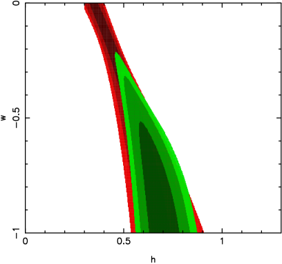
Figure 1: Likelihood contours for the (constant) Equation of State parameter $w$ (with prior $w\geq-1$) vs. the Hubble parameter $h$. The background set of contours are from using 2dFGRS+CMB and the foreground contours (at the levels of 1,2 and 3 sigma) are based on 2dFGRS+CMB+HST. From Percival et al. (2002).

4 The Alcock-Paczynski Curvature Test

Consider a spherical object at high redshift. If the wrong cosmology is assumed in interpreting the distance-redshift relation along the line of sight and in the transverse direction, the sphere will appear distorted. Alcock & Paczynski (1979) pointed out that this curvature effect could be used to estimate the cosmological constant. Phillips (1994) suggested that if the correlation function in real space is isotropic it could be used as a spherical object to measure the effect. Certain studies were less optimistic than others about the possibility of measuring this A-P effect. For example, Ballinger, Peacock and Heavens (1996) argued that the geometrical distortion could be confused with the dynamical redshift distortions caused by peculiar velocities and characterized by the linear theory parameter $\beta\equiv\frac{\Omega_{m}^{0.6}}{b}$. Their model for the distorted power spectrum $P^{S}(k_{\parallel},{\bf k}_{\perp})$ as a function of line of sight and perpendicular direction was applied by Outram et al. (2001) to a sample of 10,000 quasars from the 2dF quasar redshift survey. They found best fit values with relatively large error bars, $\beta=0.39^{+0.18}_{-0.17}$ and $\Omega_{m}=1-\Omega_{Q0}=0.23^{+0.44}_{-0.13}$ (assuming $w=-1$), and illustrated that an Einstein-de Sitter Universe can only marginally be rejected. See also Popowski et al. (1998).

Matsubara & Szalay (2002a,b) showed that the typical SDSS and 2dF samples of normal galaxies at low redshift ($\sim 0.1$) have sufficiently low signal-to-noise, but they are too shallow to detect the A-P effect. On the other hand, the quasar SDSS and 2dFGRS surveys are at a useful redshift, but they are too sparse. A more promising sample is the SDSS Luminous Red Galaxies survey (out to redshift $z\sim 0.5$) which turns out to be optimal in terms of both depth and density. Figure 2 shows the expected lowest error bounds (via Fisher matrix analysis) on the Dark Energy parameters for an Equation of State of the form $w(z)=w_{0}+w_{1}z$. This analysis is based on a galaxy counts in 15 $h^{-1}$Mpc spheres. While this analysis is promising, it remains to be tested if non-linear clustering and complicated biasing (which is quite plausible for red galaxies) would not ‘contaminate’ the measurement of the Equation of State. Even if the A-P test turns out to be less accurate than other cosmological tests (e.g. CMB and SN Ia) the effect itself is an important ingredient in analyzing the clustering pattern of galaxies at high redshifts.

A variant of the A-P method has been proposed by Hui et al. (1999) and McDonald et al. (1999) using observations of the Lyman-$\alpha$ forest in the spectra of close quasar pairs. The idea is to compare the auto-correlation along the line of sight with the cross-correlation between two (or more) close lines of sight to quasars. It has been estimated that 30 or so pairs of quasar spectra are needed to estimate of the Dark Energy parameters with reasonable accuracy, subject to modelling uncertainties.

Figure 2: Expected (minimal) error bounds on the dark energy parameters ($w_{0},w_{1},\Omega_{Q0}$) from the Luminous Red Galaxies SDSS survey. One of three parameters are held fixed. Inner ellipses represent the 1-sigma uncertainty level of one-parameter distribution function. Outer ellipses represent the 1-sigma of the joint probability distribution. The biasing parameter is held fixed (solid lines) or is marginalized over (dotted lines). From Matsubara & Szalay (2002b).

5 Abundance of Clusters and Galaxies with Redshift

A popular method for constraining cosmological parameters is to count the number $N(z)$ of clusters with redshift. Commonly the Press-Schechter mass function (or one of its variants) is used to predict the number of clusters with redshift. The Equation of State parameter is mainly sensitive to the growth rate $\delta(z)$ and the volume element (e.g. Wang & Steinhardt 1998; Weller et al. 2002). The main uncertainty is in relating the observed cluster quantities such as temperature, velocity dispersion or Sunyaev-Zeldovich effect to the cluster mass. While some empirical relations exist, they suffer from various systematic effects, e.g. evolution. The cluster abundance test is discussed in more detail by others in this Volume.

Another variant of this method has been suggested by Newman & Davis (2002) for the abundance of galaxies (e.g. in the DEEP2 survey, over the redshift range $0.7<z<1.5$ ) as a function of their circular velocity. Subject to possible systematic errors, this test can provide information about Dark Energy parameters, in particularly if extra constraints on $\Omega_{m}$ are available.

6 Cross Correlation of the CMB and Galaxy Surveys

An entirely different method to constrain Dark Energy, by cross correlating the CMB with tracers of the mass density at low redshift, has been proposed by Crittenden & Turok (1996). The idea is that in a Universe with a Cosmological Constant the gravitational potential is time dependent even on large scales (unlike in the Einstein de Sitter case, in which the potential is constant with time). Then CMB fluctuations can arise via the Integrated Sachs Wolfe (ISW) effect, as the photons travel through the time-dependent potentials. They can be observed by searching for spatial correlations between the CMB and the local matter density (e.g. from galaxy counts $N$), $<\delta N\delta T>$. Boughn & Crittenden (2002) crossed-correlated the CMB with distant radio sources, and could only place an upper limit on the cross-correlation signal. For a Cosmological Constant model ($w=-1$) they translated it to an upper limit of

$$\Omega_{Q0}\leq 0.74\;\;(95\%CL)\;.$$

This is actually the only measurement discussed in this review which argues marginally against a Dark Energy component (it is actually similar to the upper limit derived from the frequency of lensed quasars; Kochaneck 1996). However, this upper limit is still in accord with the concordance model, and systematic effects such as galaxy biasing may confuse the deduction of the cosmological parameters. If indeed a Dark Energy component does exist, it should be detectable with future CMB maps and galaxy surveys.

7 Conclusions

The main conclusions of this review are:

• The present epoch matter power spectrum and dynamics are almost ‘blind’ to a Dark Energy component. This is actually useful as these measurements can be used to deduce the matter density parameter $\Omega_{m}$ independent of any assumption on the nature of the Dark Energy, and then combined with other probes such as the CMB and Supernovae Ia.

• Geometrical tests and counts at high redshift are potentially useful, but they suffer from degeneracy with other parameters such as $\Omega_{m}$ and biasing.

• The current data are consistent with $w=-1$ (i.e. a Cosmological Constant), but other forms of Quintessence $w(z)$ are still possible.

8 Outlook

There is general acceptance (perhaps too strongly) of the ‘concordance’ model with the following ingredients: 4% baryons, 26% Cold Dark Matter (possibly with a small contribution of massive neutrinos) and the remaining 70% in the form of Dark Energy (the Cosmological Constant or ‘Quintessence’). Conceptually, it seems we have to learn to live in a multi-component complex Universe, which perhaps takes us away from an idealized model motivated by Occam’s razor.

While phenomenologically the $\Lambda$-CDM model has been successful in fitting a wide range of cosmological data, there are some open questions:

• Both components of the model, $\Lambda$ and CDM, have not been directly measured. Are they ‘real’ entities or just ‘epicycles’? Historically epicycles were actually quite useful in forcing observers to improve their measurements and theoreticians to think about better models!

• ‘The Old Cosmological Constant problem’: Why is $\Omega_{Q0}$ at present so small relative to what is expected from Early Universe physics?

• ‘The New Cosmological Constant problem’: Why is $\Omega_{m0}\sim\Omega_{Q0}$ at the present-epoch? Why is $w\approx-1$ ? Do we need to introduce new physics or to invoke the Anthropic Principle to explain it?

• There are still open problems in $\Lambda$-CDM on the small scales, e.g. galaxy profiles and satellites.

• The age of the Universe is uncomfortably close to some estimates for the age of the Globular Clusters, if their epoch of formation was late.

• Could other (yet unknown) models fit the data equally well?

• Where does the field go from here? Should the activity focus on refinement of the cosmological parameters within $\Lambda$-CDM, or on introducing entirely new paradigms?

Acknowledgements.  I am grateful to members of the 2dF galaxy redshift survey team and participants of the Leverhulme Quantitative Cosmology group in Cambridge for helpful discussions.

References

- [1] Alcock C., Paczynski B., 1979, Nature, 281, 358
- [2] Bahcall, N.A., Ostriker, J.P., Perlmutter, S., Steinhardt, P.J., 1999, Science, 284, 148
- [3] Ballinger, W.E., Peacock, J.A., Heavens, A.F., 1996, MNRAS, 292, 877
- [4] Benson A.J., Cole S., Frenk C.S., Baugh C.M., Lacey C.G., 2000, MNRAS, 311, 793
- [5] Blanton M., Cen R., Ostriker J.P., Strauss M.A., Tegmark M., 2000, ApJ, 531, 1
- [6] Boughn, S.P., Crittenden, R.G., 2002, Phys. Rev. Lett., 88, 021302
- [7] Crittenden R.G., Turok, N., 1996, Phys. Rev. Lett., 76, 575
- [8] Dekel A., Lahav O., 1999, ApJ, 520, 24
- [9] Efstathiou G. & the 2dFGRS team, 2002, MNRAS, 330, 29
- [10] Elgaroy O. & the 2dFGRS team, 2002, Phys. Rev. Lett., 89, 061301,
- [11] Freedman W.L., 2001, ApJ, 553, 47
- [12] Fry, J., 1996, ApJ, 461, L65
- [13] Hui L., Stebbins A., Burles A., 1999, ApJ, 511, 5
- [14] Kochaneck, C., 1996, ApJ, 466, 638
- [15] Lahav, O., Lilje, P.B., Primack, J.R., Rees, M.J., 1991, MNRAS, 251, 128
- [16] Lahav O. & the 2dFGRS team, 2002, MNRAS, 333, 961
- [17] Lewis A., Bridle S.L., 2002, astro-ph/0205436
- [18] Lilje, P.B., 1992, ApJ, 386, L33
- [19] Lokas, E., Hoffman, Y., 2002, astro-ph/0108283
- [20] Maor, I., Brustein, R., McMahon, J., Steinhardt, P.J., 2002, Phys. Rev. D, 65, 123003
- [21] Matarrese S., Coles P., Lucchin F., Moscardini L., 1997, MNRAS, 286, 95
- [22] Matsubara T., Szalay A., 2002a, ApJ, 574, 1
- [23] Matsubara T., Szalay A., 2002b, astro-ph/0208087
- [24] McDonald, P. et al., 1999, ApJ, 528, 24
- [25] Melchiorri, A., Mersini L., Odman C., Trodden, M., 2002, astro-ph/0211522
- [26] Newman, J.A., Davis, M. , 2002, 564, 567
- [27] Outram O.J. et al. 2001, MNRAS, 328, 174
- [28] Percival W.J. & the 2dFGRS team, 2001, MNRAS, 327, 1297
- [29] Percival W.J. et al. & the 2dFGRS team, 2002, MNRAS, 337, 1068
- [30] Phillipps, S., 1994, MNRAS, 269, 1077
- [31] Popowski, P.A. at al., 1998, ApJ, 498, 11
- [32] Peebles, P.J.E., Ratra, B., 2002, astro-ph/0207347
- [33] Sahni V., Starobinsky A., 2000, Int. J. Mod. Phys., 9, 373
- [34] Somerville R., Lemson G., Sigad Y., Dekel A., Colberg J., Kauffmann G., White S.D.M., 2001, MNRAS, 320, 289
- [35] Starobinsky A., 1998, astro-ph/9810431
- [36] Verde L. et al. & the 2dFGRS team, 2002, MNRAS, 335, 432
- [37] Wang L., Steinhardt, P.J., 1998, ApJ, 508, 483
- [38] Weller J., Battye, R., Kneissl, R., 2002, Phys Rev Lett, 88, 231301