Nanolensing of gamma-ray bursts

Abstract

All quasars vary in their optical flux on a time-scale of years, and it has been proposed that these variations are principally due to gravitational lensing by a cosmologically distributed population of planetary mass objects. This interpretation has implications for the observable properties of gamma-ray bursts (GRBs) – as a source expands across the nano-arcsecond caustic network, variability is expected – and data on GRBs can be used to test the proposed model of quasar variability. Here we employ an ultra-relativistic blast-wave model of the source, with no intrinsic variations, to study the effects of nanolensing on GRBs. Taken in isolation the light-curves of the caustic crossings are predictable, and we find that a subset of the predicted light-curves (the image-annihilating fold crossings) resemble the “pulses” which are commonly seen in long GRBs. Furthermore, for sources at high redshift the expected time between caustic crossings is of order seconds, comparable to the observed time between pulses. These points suggest that it might be possible to model some of the observed variations of GRBs in terms of nanolensing; however, our simulated light-curves exhibit a small depth of modulation compared to what is observed. This means that the GRB data do not significantly constrain the quasar nanolensing model; it also means that the simplest nanolensing model cannot explain the observed GRB “pulses”. Viable nanolensing models for pulses probably require a large external beam shear. If a viable model can be constructed it would effect a considerable simplification in source modelling and, ironically, it would explain why no macro-lensed GRBs have been identified to date.

Independent of the particular theoretical model, we can test for the presence of nanolensing in GRB data because any variability due to nanolensing should manifest parallax: the timing of caustic crossings, and hence the temporal substructure of bursts should be different as seen by separated observers. Parallax therefore shifts triangulated burst locations away from their true positions; this displacement is typically expected to be at the few arcminute level, and existing astrometry is not good enough to reveal the predicted effects. Useful constraints can, however, be obtained by comparing the relative timing of individual peaks in the light-curves recorded by spacecraft in the Inter-Planetary Network; published data show hints of the predicted temporal shifts, but the photon counting statistics are not good enough to categorically decide the matter. There is no plausible alternative interpretation for this phenomenon, and if it is confirmed as a real effect then it compels acceptance of a cosmology that is very different from the currently popular model.

1 Introduction

At present we do not know what constitutes the bulk of the material Universe, i.e. the dark matter. Many dark matter candidates have been proposed, ranging from elementary particles to macroscopic objects such as black holes – see, e.g., Trimble (1987), Ashman (1992), Carr (1994). To date it has been possible to eliminate some suggestions (e.g. brown dwarfs: Tinney 1999), by virtue of a clear conflict between models and data, but a positive identification has not been achieved. One proposal whose implications have not yet been thoroughly explored is that of Hawkins (1993, 1996), who argued, on the basis of photometric monitoring of quasars, that the Universe contains a near-critical density of planetary-mass objects (cf. Press and Gunn 1973). Gravitational lensing by such a population is capable of explaining much of the observed variability (see also Schneider and Weiß 1987; Schneider 1993) — though this should not be taken to imply that intrinsic variations are absent. This suggestion is a radical departure from the now-standard picture of a universe dominated by elementary particles (i.e. Cold Dark Matter – see, e.g., Peebles 1993; Blumenthal et al 1984; Davis et al 1985), and has received little theoretical attention. Building on earlier work (Schneider and Wagoner 1987; Rauch 1991; Seljak and Holz 1999; Metcalf and Silk 1999), Minty, Heavens and Hawkins (2001) described a statistical test of the model based on the light-curves of distant supernovae, but existing data do not allow these ideas to be usefully implemented. A test based on surface brightness variability in low-redshift galaxies has been described by Lewis and Ibata (2001), but this idea also requires data which are not yet available, as does the test based on monitoring quasars seen through low-redshift clusters of galaxies (Walker and Ireland 1995; Tadros, Warren and Hewett 1998). Data from the MACHO and EROS experiments exclude planetary-mass compact objects as a significant contributor to the Galactic dark matter (Alcock et al 1998). However objects which are sufficiently compact that they qualify as strong gravitational lenses at cosmological distances are not necessarily strong gravitational lenses when they are located in the Galactic halo (Walker 1999; see also Draine 1998, Rafikov and Draine 2001). The Galactic microlensing experiments therefore do not directly test the quasar nanolensing hypothesis.

It is obvious that one could attempt to devise further, more sophisticated tests of the nanolensing interpretation based on existing quasar data, but it is a priori unlikely that any such test will yield a definitive result. The main reason for this is source size: the low amplitude of variations seen in quasar optical light-curves means that these sources are necessarily larger than the scale-size of the hypothesised caustic structure, thus smoothing the magnification pattern, and in the process destroying the high spatial-frequency information. (This would be less of a barrier to progress if we had a reliable model for the physical structure of quasars, so that detailed predictions for their lensed appearance could be given with some confidence.) For example the approach of Dalcanton et al (1994; see also Canizares 1982), based on the statistics of equivalent widths of quasar emission lines, is quite insensitive in this regime where the continuum source is resolved by the lenses. To make progress we therefore require a numerous population of small, highly-luminous sources at large distances; gamma-ray bursters constitute such a population. Gravitational lensing of gamma-ray bursts has previously been considered by a number of authors (e.g. Paczyński 1986b; McBreen and Metcalfe 1988; Mao 1992; Gould 1992; Blaes and Webster 1992; Nemiroff and Gould 1995), but their considerations are relevant to lenses which are either much more massive, or much less massive than the planetary-mass range which we consider here. The present work also differs substantively from previous investigations in that the evolution (expansion) of the source structure plays a critical role in our analysis.

Following the launch of the Compton Gamma-Ray Observatory, BATSE (Burst And Transient Source Experiment) soon discovered that gamma-ray bursts are isotropically distributed on the sky, and that they depart from Euclidean source counts at low flux levels (Fishman et al 1994). These discoveries immediately shifted attention away from interpretations based on Galactic neutron stars, which had previously been popular, towards a variety of models in which energies amounting to a significant fraction of $\mathrm{M_{\odot}}c^{2}$ are rapidly released by sources at cosmological distances (see Paczyński 1995). Discovery of X-ray afterglows from these transient events (Costa et al 1997) by BeppoSAX allowed the sources to be accurately positioned, and thus led to the discovery of optical and radio afterglows (van Paradijs et al 1997; Djorgovski et al 1997; Frail et al 1997). Spectroscopy of these optical transients has in some cases revealed absorption lines from gas at redshifts $z_{s}\gtrsim 1$, thus firmly establishing the distance scale of the bursters to be cosmological (Metzger et al 1997; van Paradijs, Kouveliotou and Wijers 2000).

Although we still do not know what process injects the burst energy, it is broadly agreed that the radiation observed from GRBs arises from a relativistically expanding source. Relativistic expansion is required in order that we should see gamma-rays at all – at least at energies $\gtrsim$ MeV – otherwise the inferred source-size is so small, and the photon energy density so high, that two-photon pair-production converts essentially all the gammas into material particles (Cavallo and Rees 1978; Fenimore, Epstein and Ho 1993; Baring and Harding 1997). These considerations require expansion with Lorentz factors of at least $\Gamma\sim 10^{2}$.

At an early stage in the modelling of gamma-ray bursts in a cosmological context, it was pointed out that gamma-ray emission should arise as the the ambient medium undergoes shock compression by the expanding material (Rees & Mészáros 1992). This picture – the “blast-wave”, or “external shock” model – now provides the accepted context for modelling the broad-band (X-ray, optical and radio) afterglows of bursts (Paczyński and Rhoads 1993; Mészáros and Rees 1997; Granot, Piran and Sari 1999), but has fallen into disfavour as an interpretation of the prompt gamma-ray burst. The reason for the demise of this model is simply that it cannot, in itself, accommodate the rapid, large-amplitude variability which is manifest in the gamma-ray data (Fenimore, Madras and Nayashkin 1996; Sari and Piran 1997; see also Dermer and Mitman 1999; Fenimore, Ramirez-Ruiz and Wu 1999). This point has promoted the idea that the gamma-rays arise from internal shocks within the relativistic outflow, so that the temporal variations of the burst reflect the input power variations of the source (e.g. Rees and Mészáros 1994; Kobayashi, Piran and Sari 1997).

Because we are investigating an hypothesis in which apparent variability arises external to the source, as a result of gravitational lensing, arguments which assume that the observed variations are intrinsic immediately lose most, if not all of their force. Given this there are at least three motivations to return to the blast-wave interpretation of the prompt gamma-ray emission: first, this picture allows the initial deposition of energy to be impulsive, and is therefore suitable for a broad range of source models (independent of the specific physics of the energy input) with no fine-tuning required; secondly, the low radiative efficiency of internal shocks (Spada, Panaitescu and Mészáros 2000) appears to be inconsistent with the event energetics in at least some cases (Paczyński 2001); and thirdly, gamma-ray emission from an external shock ought to be present at some level. This emission can be sensibly described by a self-similar, decelerating blast-wave model, similar to those developed for the afterglow emission (e.g. Granot, Piran and Sari 1999), but radiative rather than adiabatic. Such a description leads us to expect a circular source with very strong limb brightening and consequently we anticipate significant flux variations if the limb crosses a caustic. This thin, bright and rapidly expanding ring is a near-perfect instrument for revealing any caustic structure that might be present along the line-of-sight to the source — see also Loeb and Perna (1998), and Mao and Loeb (2001), who considered microlensing of optical afterglows by stellar-mass objects in the low optical-depth limit.

In this paper we use the source model just described to explore the hypothesis that the Universe contains a high density of planetary-mass objects, with an optical depth to gravitational lensing of order unity. Often the characteristic angular scale of the lenses (in arcseconds) is indicated in the nomenclature given to associated phenomena (e.g. microlensing), and following this convention dictates the name “nanolensing” for the effects discussed herein. Although gravitational lensing is the main focus of our attention here, in studying the variations which might be introduced by this process we are also implicitly addressing the physics of the sources themselves. We start by presenting our source model in §2, and in §3 we turn to aspects of the gravitational lensing; light-curves which result from the marriage of these elements are presented and compared with data in §4. The role of parallax is explored in §5, followed by a discussion of related issues concerning both the lenses and the sources (§6), and our conclusions are given in §7.

2 Source model

Following Rees and Mészáros (1992), we adopt a spherically-symmetric, ultra-relativistic blast-wave model of the gamma-ray burst phenomenon, in which a total energy of $10^{52}\,E_{52}\;{\rm erg}$ resides in ejecta which expand with an initial Lorentz factor $\gamma=10^{3}\gamma_{3}\gtrsim 10^{3}$ into a homogeneous medium of density $n\;{\rm cm^{-3}}$. At first the ejecta coast ($\gamma\simeq$ constant), but this lasts only for a brief period $\sim 0.1\;\gamma_{3}^{-8/3}(E_{52}/n)^{1/3}\;{\rm s}$, and subsequently the ejecta decelerate, with some fraction of the thermalised power appearing as radiation. We will treat these as distinct, self-similar phases of evolution, characterised by the index $m$, where

$$\Gamma^{2}=\Gamma_{0}^{2}\left({{R_{0}}\over{R}}\right)^{m}$$ (1)

at radius $R$, and $\Gamma=\sqrt{2}\gamma$ is the Lorentz factor of the shock-wave which precedes the ejecta (Blandford and McKee 1976). In the coasting phase we evidently have $m=0$; while $m=3$ for adiabatic evolution, and $m=12$ for a fully radiative blast-wave – i.e. one in which all of the thermalised energy is promptly radiated away (Cohen, Piran and Sari 1998). The adiabatic approximation is appropriate for the afterglow, when the radiation time-scale is much longer than the expansion time-scale; for the gamma-ray burst itself we adopt the fully radiative solution, $m=12$. In this circumstance the gamma-rays arise from a thin shell immediately behind the shock front.

It is convenient to take $R_{0}$ as the radius at which the transition between coasting and semi-radiative solutions takes place, and to model the evolution of the blast wave as if there were an instantaneous transition between these solutions, as the shock crosses this radius. We can estimate the value of $R_{0}$ by noting that the shock will start to decelerate when a significant fraction of the initial energy of the blast has been thermalised (Rees and Mészáros 1992):

$$R_{0}\simeq 1.2\times 10^{16}\left({{E_{52}}\over{n\Gamma_{3}^{2}}}\right)^{1/3}\qquad{\rm cm}.$$ (2)

Where numerical estimates are required we adopt the values $E_{52}=\Gamma_{3}=n=1$ throughout. For some estimates we need to know, in addition, the Hubble constant, which we take to be $H_{0}=70\;{\rm km\,s^{-1}\,Mpc^{-1}}$.

In this paper we consider only bolometric radiation properties, so that it is not necessary to specify the radiation mechanism.

2.1 Kinematics

Because the expansion is spherically-symmetric, the observed source structure is axisymmetric, and at any given time it can be expressed as a function of a single variable, such as the apparent radius, $r$, as measured by a distant observer, relative to the line-of-sight to $R=0$. Because the expansion is relativistic, it is essential to incorporate light travel-time in any computation of the appearance of the source. In terms of the time, $t$, measured by a distant observer at the same redshift (with $t=0$ corresponding to the start of the expansion), there is a maximum apparent radius, $r_{max}$, from which photons can be received by the observer:

$$r_{max}^{2m+2}=\Gamma_{0}^{2}R_{0}^{m}\left[\left({{2m+2}\over{m+2}}\right)ct\right]^{m+2},$$ (3)

and this defines the limb of the source at any time. In general we expect the source to be at non-zero redshift, $z_{s}$, and to allow for this one simply makes the replacement $t\rightarrow t/(1+z_{s})$, both here and in subsequent formulae. In cases where a numerical estimate is required, we adopt the value $z_{s}=5$ throughout this paper; this corresponds to the median redshift in the GRB source population model of Bromm and Loeb (2002). The radius at $r=r_{max}$ is given by $R_{max}$:

$$R_{max}^{m+1}=2ct\,\Gamma_{0}^{2}R_{0}^{m}\left({{m+1}\over{m+2}}\right),$$ (4)

and if we define $q\equiv R/R_{max}$, then for any point on the emitting surface, at any given time, we have

$$\tilde{r}^{2}={q\over{m+1}}\left[(m+2)-q^{m+1}\right],$$ (5)

where $\tilde{r}\equiv r/r_{max}$. Notice that there are two values of $q$ which correspond to each value of $\tilde{r}$ (other than $\tilde{r}=1$); one of these values lies in the range $0\leq q<1$, while the other lies in the range $1<q\leq Q$, with $Q^{m+1}=m+2$.

Knowing the apparent size of the source as a function of time, we can easily find the apparent expansion speed, $\beta_{ap}$ (in units of $c$), just by differentiating equation 3:

$$\beta_{ap}^{2m+2}=\Gamma_{0}^{2}\left[{{(m+2)R_{0}}\over{(2m+2)ct}}\right]^{m}.$$ (6)

2.2 Intensity profile

By virtue of being almost coincident with the shock front, the emitting surface exhibits the geometry of a shell moving with Lorentz factor $\Gamma$, as described in §2.1. However, the emitting particles are part of the post-shock flow so their bulk Lorentz factor is $\gamma=\Gamma/\sqrt{2}$, and in consequence the limb of the source ($\tilde{r}=1$) does not correspond to the peak of the observed intensity. This point does not appear to have been recognised previously (cf. Granot and Loeb 2001; Gaudi, Granot and Loeb 2001). For a thin emitting shell, the peak surface brightness corresponds to polar angle $\psi=\pi/2$ (as measured in the co-moving frame) relative to the surface normal. For an emitting shell of fractional radial thickness $\Delta\ll 1$, the bolometric surface brightness can be described by

$$I(r,t)={{{\cal D}^{4}\,{\cal I}}\over{\sqrt{\cos^{2}\psi+\Delta/4}}},$$ (7)

with ${\cal I}$ being the bolometric intensity emitted normal to the surface, as measured in the rest frame of the emitting shell, and ${\cal D}$ the Doppler factor. (Recall that $q(\tilde{r})$ is double-valued, so that there are implicitly two contributions to the right-hand-side of equation 7.) It is easy to show that rays reaching the observer at a given instant satisfy

$$\cos\psi={{(2m+3)q^{m+1}-(m+2)}\over{(2m+1)q^{m+1}+(m+2)}},$$ (8)

and that the ratio of observed-to-emitted photon energies is

$${\cal D}={{4(m+1)\gamma_{max}q^{(m+2)/2}}\over{(2m+1)q^{m+1}+(m+2)}},$$ (9)

where $\gamma_{max}\sqrt{2}:=\Gamma_{0}(R_{0}/R_{max})^{m/2}$. Now the total energy density in the post-shock gas is just $4\gamma^{2}n\,m_{p}c^{2}$ (Blandford and McKee 1976), and in the frame of this material the shock itself moves at speed $c/3$, so if all of this power is promptly radiated, the emergent normal intensity (i.e. at $\psi=0$) is

$${\cal I}\simeq{1\over{3\pi}}\gamma^{2}n\,m_{p}c^{3}.$$ (10)

The above set of equations provides a complete prescription for calculation of the bolometric intensity profile; the fully radiative case, corresponding to $m=12$, is shown in figure 1 for a fractional shell thickness of $\Delta=4\times 10^{-3}$. This choice for $\Delta$ is appropriate to, for example, synchrotron emission at $\sim 200$ keV if the magnetic field energy-density is 10% of the equipartition value. The essential feature of this profile is that it is very strongly limb-brightened, with a sharp peak at $r\simeq 0.99295\,r_{max}$ (corresponding to $q^{m+1}:=(m+2)/(2m+3)$, i.e. $\psi=\pi/2$). Source intensity profiles for any index $3\leq m\leq 12$ exhibit this limb-brightening effect, but as $m$ increases the limb-to-centre intensity ratio grows according to $(32/27)(m+2)^{3m/(m+1)}$, and the peak-to-centre intensity ratio equals $(2m+3)^{3m/(m+1)}/8\sqrt{\Delta}$; the peak also shifts to larger radii with increasing $m$.

The received flux is computed in the usual way, i.e.

$$F=\int\!\!{\rm d}\Omega\,I\quad\propto\quad 2\pi r_{max}^{2}\int_{0}^{1}\!\!{\rm d}\tilde{r}\,\tilde{r}\,I.$$ (11)

Using equation 5 it is straightforward to rewrite the integral over $\tilde{r}$ as an integral over $q$ such that $0\leq q\leq Q$. In this way we find that the observed flux should vary as $F\propto t^{(2-m)/(m+1)}$, so that $F$ grows as $t^{2}$ during the early, coasting phase ($m=0$), and then declines as $t^{-10/13}$ during the self-similar radiative ($m=12$) evolution. A simple model light-curve can thus be constructed by applying these two solutions in their appropriate regimes (small/large $t$, respectively), and switching between the two at the point where they cross. That is the procedure we shall follow here — our calculations are intended to be illustrative and high precision is not needed. One important point to note is that the luminosity in the self-similar deceleration phase declines too slowly to yield a finite radiated energy at late times, and so the model clearly has a limited range of applicability.

Figure 1: The radial distribution of bolometric intensity, for a blast-wave in self-similar, fully-radiative ($m=12$) evolution. The emitting shell is assumed to have a fractional radial thickness $\Delta=4\times 10^{-3}$. The intensity is normalised to the central intensity, and declines monotonically beyond the left-hand edge of the plot. The location of the peak ($\tilde{r}\simeq 0.993$) corresponds to $\psi=\pi/2$, i.e. tangent to the emitting shell.

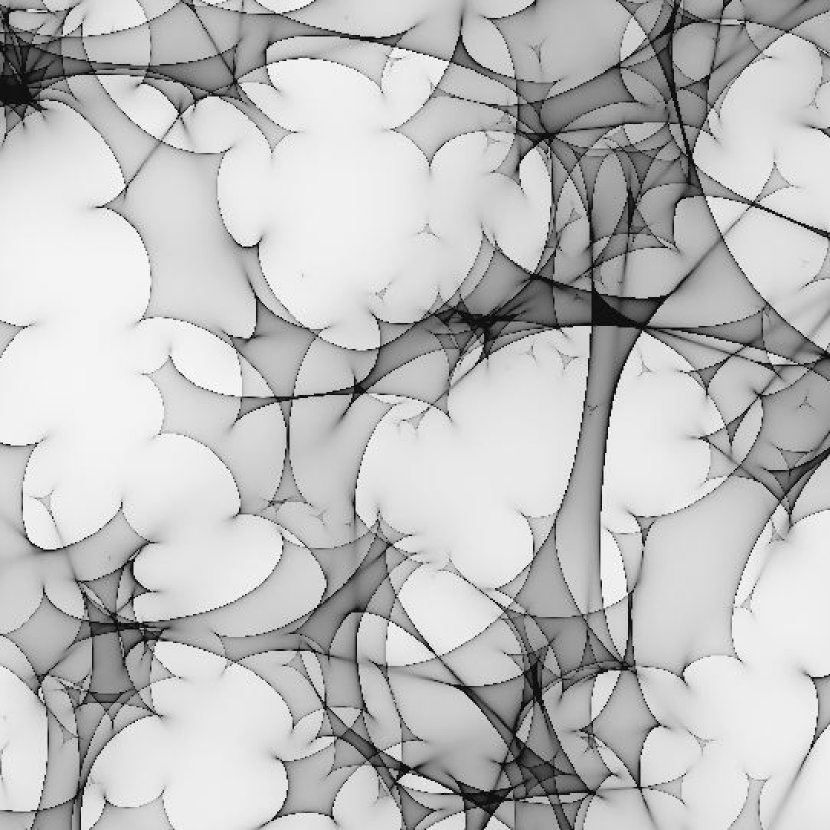
Figure 2: One realisation of a magnification pattern appropriate to a source at redshift $z_{s}=5$, in a universe populated with point-mass lenses such that $\Omega_{lens}=\Omega=1$. This pattern is derived from a simulation in which the locations of the lenses are chosen randomly within a single plane, having a total optical depth of 0.6. The rays are chosen to have a uniform density across the image plane; this figure shows their density across the source plane; regions of high ray density in this figure are therefore areas of high magnification, and most of these regions correspond to fold caustics. Our simulations utilised code from Wambsganss, Paczyński & Katz (1990).

Figure 3: The images (solid lines) of two thin (10% fractional width), annular sources (dashed curves), on either side of a fold caustic (dotted line). For convenience the critical curve ($X=0$) has been superimposed on the caustic ($x=0$). The upper half of this figure is the three-image region, and the lower half is the single-image region. In each case the inner boundary of the annulus just touches the caustic, and the centre of each source is assumed to lie at a distance of $s=\pm 1/a$ from the fold.

3 Lens model

If the Universe contains a mean mass density in lenses $\Omega_{lens}$ (in units of the critical density), then the optical depth to gravitational lensing is $\tau\simeq 0.11\,\Omega_{lens}$ for a source at redshift $z_{s}=1$, and $\tau\simeq 0.62\,\Omega_{lens}$ for a source at redshift $z_{s}=5$ (Turner, Ostriker and Gott 1984). These results are for a universe with a mean total density of $\Omega=1$ (the Cosmological Constant, $\Lambda=0$), and for a given redshift the ratio $\tau/\Omega_{lens}$ increases as $\Omega$ decreases. The study by Schneider (1993) demonstrated that $\Omega_{lens}\sim 0.5$ is required (see his figure 6b) if the variability reported by Hawkins (1993) is attributed to gravitational lensing. The nanolensing interpretation of quasar variability is also consistent with the currently favoured combination of cosmological model parameters ($\Lambda\simeq 0.7$, $\Omega\simeq 0.3$) provided that essentially all of the matter is in the form of lenses, i.e $\Omega_{lens}\simeq 0.3$ (Minty 2001). The details of the cosmological model are unimportant here; for simplicity of calculation we have therefore adopted a model universe with $\Omega_{lens}=\Omega=1$.

The magnification pattern which is introduced by the lenses takes the form of a caustic network, in which the appearance of any source is influenced by a large number of lenses (Paczyński 1986a); an example of such a network is shown in figure 2. In this figure we see a large number of fold caustics – a fold is the lowest order catastrophe, at which two images merge – joined by cusps (catastrophes where three images merge). In the present paper we illustrate the effects of GRB nanolensing through analytic and numerical calculations of a source crossing a single fold caustic (this section). We then (§4) simulate the global lightcurves expected for a source expanding across a caustic network such as that shown in figure 2.

In the immediate vicinity of a fold caustic the mapping between rectangular source coordinates $(x,y)$, and image coordinates $(X,Y)$, is well approximated by a quadratic form (see Schneider, Ehlers & Falco 1992):

$$x={1\over 2}aX^{2},\qquad y={1\over 2}Y,$$ (12)

with the $x$ axis oriented perpendicular to the caustic, and the curvature, $a$, being a positive constant. Here the factor $1/2$ in the $x\leftrightarrow X$ mapping is arbitrary (because $a$ remains unspecified), but the factor of $1/2$ in the $y\leftrightarrow Y$ mapping is required in order that the fold be convergence free – a pure shear lens mapping – as all empty-beam lens mappings must be in General Relativity. There are two solutions (images) to these equations for any source located at $x>0$, and it is straightforward to determine their magnifications:

$$\mu_{\pm}=\pm{{1}\over{2\sqrt{2ax}}}.$$ (13)

In addition to this image pair, there will typically be a large number of other images present, but the observed flux variations around the time of caustic crossing are completely dominated by the two very bright images which are described by equations 12 and 13. If a burst occurs at any location $x<0$, then neither of these two images will be present until the source expands so as to touch the caustic, at which point the observed flux will rise abruptly. On the other hand, if a burst occurs at $x>0$ then both images will be present at all times.

There are two separate cases which we must consider, depending on which side of the caustic the burst occurs. For a point source at $x<0$ there are $2n+1$ images, whereas for $x>0$ there are $2n+3$; we therefore denote these two regions as the one-image and three-image regions, respectively, with the understanding that there are many more images present, but only the pair created/annihilated at $X=0$ is of interest here. If the source takes the form of a thin ring, as is approximately the case for the model we have adopted (§2; see figure 1), then the lensed images appear as shown in figure 3. In our subsequent development we denote the $x$ coordinate of the origin of the burst by $s$, so that the sign of $s$ determines whether one or three images are initially present.

3.1 Burst in single-image region ($s<0$)

Because the source intensity distribution is axisymmetric, it is useful to consider the properties of an infinitesimally-thin ring, radius $r$, of uniform surface-brightness, under the mapping given by equation 12. If the burst occurs at $s<0$, then images of the source first appear when the source reaches a radius $r=|s|$, and for $r>|s|$ the total magnification of the ring (summed over both images) is given by

$$\mu_{1}={{1}\over{\pi}}\sqrt{{u}\over{ar}}\;{\cal F}(\phi|u)$$ (14)

where ${\cal F}$ denotes the Incomplete Elliptic Integral of the first kind; $\cos 2\phi:=-s/r$, and $u\equiv 2r/(r+s)$. Here “magnification” means the total area occupied by the two images of the annulus, divided by the area of the annulus itself. Simple approximations to this exact result are available: $\mu_{1}\simeq(1-3\epsilon/8)/2\sqrt{a|s|}$ for $0<\epsilon\ll 1$, where $\epsilon\equiv r/|s|-1$; and $\mu_{1}\rightarrow{\cal K}(1/2)/\pi\sqrt{ar}$ for $r\rightarrow\infty$, where ${\cal K}$ is the Complete Elliptic Integral of the first kind, and ${\cal K}(1/2)\simeq 1.8541$. The exact form of the magnification, given by equation 14, is graphed in figure 4 for the case $s=-1/a$.

3.2 Burst in three-image region ($s>0$)

For a burst which occurs in the three-image region ($s>0$), the total magnification of an annulus is given by

$$\mu_{3}={{1}\over{\pi}}\sqrt{{u}\over{ar}}\;{\cal K}(u)$$ (15)

for $r<s$. On the other hand for $r>s$ we have (as with eq. 14)

$$\mu_{3}={{1}\over{\pi}}\sqrt{{u}\over{ar}}\;{\cal F}(\phi|u).$$ (16)

Simple approximations can be found for these expressions in the following regimes: $\mu_{3}\simeq 1/\sqrt{2as}$, for $r\ll s$; $\mu_{3}\simeq\ln(32/|\epsilon|)/2\pi\sqrt{as}$, where $|\epsilon|\ll 1$ (and $\epsilon=r/s-1$); and $\mu_{3}\simeq{\cal K}(1/2)/\pi\sqrt{ar}$ for $r\rightarrow\infty$. The exact results are shown in figure 4, for the case where $s=1/a$, alongside the corresponding magnification curve for a burst occurring in the single image region.

3.3 The median lens

For some purposes (e.g. estimating a characteristic length scale in the source plane) it is important to know whereabouts on the line-of-sight the typical lens is located. This need is most sensibly addressed by determining the redshift at which the optical depth to gravitational lensing is one half of the total optical depth for the source under consideration. Using equation 2.13b of Turner, Ostriker and Gott (1984) this can be quite straightforwardly achieved, and the result is that for a source at redshift $z_{s}$ the median lens is located at redshift $\langle z\rangle$:

$$\langle 1+z\rangle=\sqrt{1+z_{s}}.$$ (17)

Thus for a source at redshift $z_{s}=3$ the median lens redshift is unity, and at low redshift ($z_{s}\ll 1$) the median lens is located half-way to the source.

One application of the foregoing is the relationship between transverse dimensions measured in the source plane and in the observer’s plane. Appropriate angular-diameter distances for our circumstance are evidently “empty-beam”, distances (for $\Omega=1$), and these are given in table 1 of Turner, Ostriker and Gott (1984). Denoting observer-lens and lens-source angular-diameter distances by $D_{d}$ and $D_{ds}$, respectively, we introduce the “lever arm”, $\varpi\equiv D_{ds}/D_{d}$. It is this ratio which, for any given lens, determines the relationship of a transverse distance in the source plane to the corresponding distance in the observer’s plane. It is straightforward to show that the median lever arm (i.e. the lever arm of the median lens) is

$$\langle\varpi\rangle=(1+z_{s})^{-3/4},$$ (18)

and we will make use of this result in §5.

3.4 Variability time-scale

In combination with our kinematic model of the source structure (§2.1), the statistical properties of the caustic network determine the predicted variability time-scale of GRBs as a function of source redshift and lens mass. At each occasion when the limb of the source crosses a caustic, a peak is introduced into the light-curve, so the characteristic time-scale between peaks is just the time taken by the source to expand in area by $1/\Sigma$, where $\Sigma$ is the number of caustics per unit area in the source plane. In the low optical depth regime there are four folds in each projected Einstein Ring. At high optical depth, where a caustic network develops, the caustic density is higher by a factor equal to the mean magnification, $(1-\tau)^{-2}$, and we therefore estimate the caustic density by $\Sigma\sim 4\tau/(1-\tau)^{2}$ per unit Einstein Ring area in the source plane. The circumstance $\tau=1$ corresponds to $z_{s}\simeq 10.7$ in our model universe, and the caustic density becomes very large, and variability time-scale correspondingly short, for sources around this redshift.

Using our self-similar ($m=12$) source model, we can now estimate the expected variability time-scale, $t_{var}$ via

$$t_{var}^{-1}\sim\Sigma{{\rm d\ }\over{{\rm d}t}}\;\pi r_{max}^{2}.$$ (19)

It is worth noting that $r_{max}^{2}\propto t^{(m+2)/(m+1)}$ (see eq. 3), so that the apparent area of the source increases nearly linearly with time, and the variability time-scale is thus not expected to evolve significantly during a burst. The results are shown in figure 5 as a function of lens mass, for two different values of the source redshift ($z_{s}=1,5$), and an initial Lorentz factor $\Gamma_{0}=10^{3}$. Considering that bursts may last up to several hundred seconds, and that the available temporal resolution is below 100 ms in existing data, almost the entire temporal range in figure 5 is open to study. We thus recognise that a cosmological population of planetary-mass lenses should introduce variability to gamma-ray burst profiles, suggesting a powerful test of the nanolensing interpretation of quasar variability.

The model does not make a precise prediction for the time-interval between caustic crossings, because the appropriate lens mass is not tightly constrained (nor indeed are the parameters of the source, such as $\Gamma_{0}$). Hawkins (1993) initially gave an estimate of $10^{-3}\mathrm{M_{\odot}}$, but Schneider’s (1993) analysis clearly favours $10^{-4}\mathrm{M_{\odot}}$ or even smaller values. Using three-dimensional ray shooting simulations, Minty (2001) finds that these data suggest lens masses of $10^{-5}-10^{-4}\mathrm{M_{\odot}}$. Referring to figure 5, if we adopt $\Gamma_{0}=10^{3}$ and lens masses of order $10^{-5}\mathrm{M_{\odot}}$, then the variability time-scale is expected to be $\sim 60$ seconds for a source at redshift $z_{s}\simeq 1$, and $\sim 4$ seconds for a source at $z_{s}\simeq 5$.

4 Light curves

We have taken two distinct approaches to the study of lensed light-curves: detailed calculation of the behaviour around the time of a fold-caustic-crossing event, exhibiting the type of profiles which are expected for individual “pulses” (cf. Norris et al 1996); and simulation of light-curves for GRBs seen through a caustic network. For any given burst the latter reflects the random structure of the caustic network in the vicinity of the source. We note here that the propagation times for the various images in our model differ only by amounts $\lesssim 1$ ns, and this is negligible for our purposes.

4.1 Individual “pulses”

Making use of the source intensity profile computed in §2, and the magnification curves derived in the previous section, it is now a straightforward exercise to compute the flux history, $F(t)$, from

$$F(t)\propto\int\!\!{\rm d}r\,2\pi\,r\,I(r,t)\,\mu,$$ (20)

where the total magnification, $\mu$, can be written as the sum of the “unlensed” images (actually, a large number of lensed images whose total flux is roughly constant over the time-scale of the caustic crossing), plus the bright pair of images associated with the fold caustic under consideration: $\mu=1+\mu_{1,3}$. (The choice of unity for the constant term in this relation is somewhat arbitrary.) As with equation 11, this formula can easily be rewritten as an integral over the variable $q$. After substituting for $I(r,t)$ (equations 7–10) and $\mu_{1,3}$ (equations 14–16) it is straightforward to evaluate equation 20 numerically; to do this we used the Mathematica software package. The results are shown in figure 6, for bursts occurring in both one- and three-image regions. For these calculations we have assumed $|s|=1/a$, and we have taken the fractional radial thickness of the emitting shell to be $\Delta=4\times 10^{-3}$. For each light-curve, the limb of the source first touches the caustic at $t=1.5$ seconds (an arbitrary choice).

Figure 4: The magnification of an infinitesimally-thin, annular source, of radius $r$, centred on $x=s$, under the mapping given in equation 12; this mapping describes a pure shear fold caustic at $x=0$. Here we have assumed that the curvature of the lens mapping near the fold is $a:=1/|s|$. The upper curve corresponds to $s>0$ (burst occurs in three-image region), and the lower curve corresponds to $s<0$ (burst in single-image region).

Figure 5: The nanolensing variability time-scale, in a Universe with $\Omega_{lens}=\Omega=1$, as a function of lens mass. The source is assumed to be in self-similar, fully-radiative ($m=12$) evolution with initial Lorentz Factor $\Gamma_{0}=10^{3}$; other parameters characterising the expansion have been fixed at $E_{52}=1$, and $n=1$. The solid line corresponds to a source at redshift $z_{s}=1$, while the dashed line is for $z_{s}=5$.

Figure 6: Bolometric $\gamma$-ray light-curves for a relativistic, fully-radiative ($m=12$), self-similar blast-wave seen expanding across a fold caustic. The thickness of the radiating shell is taken to be $\Delta=4\times 10^{-3}$, and the centre of expansion of the burst is assumed to be a distance $1/a$ from the fold, where $a$ is the curvature of the lens mapping. The upper curve corresponds to a burst in the three-image region, while the lower curve is for an event in the single-image region; caustic crossing occurs at $t\simeq 1.5$ s.

Some aspects of figure 6 require immediate comment. The difference in overall normalisation of the two curves at early times simply reflects the ratio of total magnifications at the onset of the burst – see figure 4 – roughly $(1+1/\sqrt{2})/(1+0)\simeq 1.7$. This property is a direct result of the simple lens model we have adopted (i.e. the quadratic relationship between source and image coordinates), and it should be remembered that this approximation is accurate only in the immediate vicinity of the caustic. Consequently it is the behaviour seen in the light-curves around $t=1.5$ s which is of prime interest, rather than the global properties. The essential features to note are, therefore, that: (i) the presence of a fold caustic introduces a significant peak into the light-curve, close to the time at which the limb of the source first touches the caustic, and (ii) this peak can be either cuspy, and approximately time-symmetric, or rounded and asymmetric. These features could, in fact, have been anticipated simply by examining the magnification profiles shown in figure 4, bearing in mind that the source structure is basically just a thin ring (figure 1).

4.2 Simulated light-curves

Although the circumstance we are considering is one in which a population of gravitational lenses is distributed along the entire line-of-sight, we have made use of simulations which are two-dimensional, with all of the lenses located in a single plane. This is partly because three-dimensional ray-tracing simulations are much slower than their two-dimensional counterparts, but mainly because a well-tested two-dimensional code was available to us (Wambsganss, Paczyński & Katz 1990). Two extensions of this code were required for our purposes: convolution of the magnification map with our model source intensity profile (§2); and a progressive “zoom” which recomputes the magnification map on larger scales as the source expands. The latter feature was implemented with an incremental “zoom” factor of 1.2, and our computational grid was 2048 pixels on a side, so that our source radius was in the range 800 to 1000 pixels. Despite this our resolution is only just adequate for the task, as the reader can easily verify by examining the radial width of the source intensity distribution (figure 1). An estimate of the Full-Width at Half-Maximum (FWHM) of the source intensity peak can be obtained from

$${\rm FWHM}\;\simeq\left({{m+2}\over{2m+3}}\right)^{(m+2)/(m+1)}{{2\sqrt{3\Delta}}\over{2m+3}},$$ (21)

and for $m=12$, $\Delta=4\times 10^{-3}$ this yields (coincidentally) ${\rm FWHM}\simeq 4\times 10^{-3}$. With a source radius of 800 pixels the intensity profile is thus 1.5 times over-sampled.

Figure 7: Simulations of the mean magnification (panel a) and resulting light-curve (panel b) for a GRB occurring at redshift $z_{s}=1$, in a universe full of nanolenses ($\Omega=\Omega_{lens}=1$); each lens is assumed to have a mass of $10^{-8}\;{\rm M_{\odot}}$. The apparent time-scale of the transition between coasting and radiative phases is given by $(1+z_{s})\,R_{0}/c\Gamma_{0}^{2}$, and for our adopted burst parameters ($E_{52}=n=\Gamma_{3}=1$) this corresponds to $0.39\,(1+z_{s})$ s. This time-scale defines the location of the peak of the burst in panel (b). Note that the magnification is in units of the theoretical average, $\left<\mu_{th}\right>=(1-\tau)^{-2}$, which, for this case, is 1.26.

Figure 8: As figure 7, but for a source redshift of $z_{s}=5$ (corresponding to the burst peak at $t=2.3$ s), and lenses of mass $10^{-5}\;{\rm M_{\odot}}$. Again, the magnification is in units of the theoretical average, $\left<\mu_{th}\right>=6.9$.

To illustrate the type of lightcurves which might be expected, we have undertaken simulations for sources at redshift $z_{s}=1$ and $z_{s}=5$, corresponding to optical depths to gravitational nanolensing of $\tau=0.11$ and $\tau=0.62$, respectively. The results of these simulations are shown in figures 7 and 8, for lenses of mass $10^{-8},10^{-5}\;{\rm M_{\odot}}$, respectively. Because the source evolves in a self-similar (scale-free) manner, it is not necessary to recompute magnification curves when the adopted lens mass is changed: different lens masses simply require a rescaling of the time axis in panel (a) of these figures, thus changing the characteristic time-scale of any variability, but not its amplitude. The choice of lens mass was made, for each of the two redshifts, so as to maximise the variability within each of the synthetic bursts.

All of our simulations follow the same basic pattern: starting from an initial magnification which is below unity, the mean magnification (i.e. average magnification over the whole source) exhibits rapid variability, the amplitude of which decreases as the source expands. These features are readily understood. Initially the source is likely to be demagnified, because most of the area of the source plane is occupied by regions with magnification below unity. Subsequently, as the source expands across the caustics, variability is seen. However, accompanying the increase in source radius, is an increase in the thickness of the high intensity ring and the modulation of the mean magnification of the source is consequently reduced. Simultaneously the time-averaged magnification trends towards its large-scale average value as the source covers an increasing area.

There are two important points which are evident on examining figures 7 and 8. First, the time-scale of the variations in the simulated light-curves is in broad agreement with the rough estimates given in §3.4 (see figure 5). Secondly, the depth of modulation seen in our simulated magnification curves is quite small, being typically of order 10%, and in the light-curves themselves, where the secular evolution is strong, it is not always apparent that the flux is varying on short time-scales.

4.3 Comparison with observations

Many high-quality gamma-ray burst light-curves were acquired by the BATSE experiment on the Compton Gamma-Ray Observatory (e.g. Fishman et al 1994), and the substructure within these light-curves has been analysed by Norris et al (1996: N96), in the case of long, bright bursts. The principal conclusion of this analysis was that these bursts can be regarded as being made up of a number of “pulses” having a typical separation of order one second (but which are not periodic). N96 found that the typical pulse shape is cuspy, similar to the peak near $t\simeq 1.5$ s in the top curve in figure 6.

Comparing these findings to the results of §§3,4, we can identify three key points. First, the observed time-scale of order one second between “pulses” is comparable to the predicted time-scale (§§3.4,4), but only if the lenses have low mass ($\sim 10^{-8}\;{\rm M_{\odot}}$), or the sources are at high redshift. Secondly, the typical “pulse” shape observed by N96 is similar to the $3\rightarrow 1$, i.e. image-annihilating, caustic crossing discussed in §3.2, and shown in figures 4 and 6. However, the theory presented earlier in this paper gave no reason to suppose that $3\rightarrow 1$ crossings should be preferred over $1\rightarrow 3$ crossings, and in fact one does expect both to be present. Both are present in the simulated light-curves shown in figures 7 and 8. One could appeal to an observational bias which favours $3\rightarrow 1$ caustic crossings over their $1\rightarrow 3$ counterparts, because the high and cuspy peaks of the former render them more visible in the light-curves (see, particularly, figure 4). However, this does not seem to us to be a strong argument. Finally, although the single fold-crossing events modelled in §3 are obvious in the light-curves, it is plain that the simulations in §4 do not yield sufficient modulation to be able to explain the profound variations seen in the data.

On the last of the above points we note that there is no discrepancy between the calculations undertaken in §3 and the simulations of §4. The difference between the computed modulation depth in the two cases simply reflects the fact that the caustics present in the simulations exhibit more curvature in the lens mapping than was assumed in §3.

5 Parallax

A key aspect of the lensing model we are investigating here is that of parallax. The importance of parallax phenomena depends on the spatial separation of the detectors which are employed, in comparison with the spatial scale on which the magnification pattern changes. In the low optical depth regime, the latter scale is given by

$$\left[4{{GM}\over{c^{2}}}{{D_{s}D_{d}}\over{D_{ds}}}\right]^{1/2}\simeq 60\sqrt{M_{-4}}\quad{\rm AU},$$ (22)

where $D_{s}$ is the angular-diameter distance of the source from the observer, and to arrive at the numerical result we have assumed $z_{s}=3$ and considered the median lens. Hence for detectors separated by a few Astronomical Units, parallax might be expected to show up only for lenses of mass $M\lesssim 10^{-7}\mathrm{M_{\odot}}$ (Nemiroff and Gould 1995). However, in the model we are considering the expanding source crosses caustics, and in the vicinity of caustics the magnification pattern varies significantly on spatial scales much smaller than given by equation 22. Indeed at caustic crossings the transverse flux gradient is limited only by the source structure, and parallax may be observable even over very modest baselines. Specifically, if the width of the high intensity ring of the source is taken to be $4\times 10^{-3}$ of the apparent radius (see §4.2), and the latter is approximately 6 AU at $t=10$ seconds ($E_{52}=n=\Gamma_{3}=1$), then parallax may be evident over transverse length scales as small as $4\times 10^{11}$ cm. In this circumstance the main instrumental requirement is for good temporal resolution in the detectors, and high signal-to-noise ratio, so that the times at which caustic crossings occur can be precisely determined (Grieger, Kayser and Refsdal 1986; Hardy and Walker 1996). Gamma-ray bursts are typically recorded with temporal resolution of tens of milliseconds, or better, often at high signal-to-noise, so that the available timing precision is generally rather good. Moreover, we wish to emphasise that, provided there are significant increases in flux associated with a caustic crossing, the ability to precisely time such an event is essentially independent of lens mass and this parameter does not influence the detectability of the two parallax phenomena we shall describe.

5.1 Displaced burst locations

Suppose we observe a burst with a pair of identical detectors whose spatial separation is small in comparison with the scale on which the lens magnification pattern changes. The caustic network will appear very similar as seen from the two different locations, but with a slight shift on the sky in a direction parallel to the sky-projection of the vector separation between the detectors, $\vec{b}_{12}=\vec{x}_{1}-\vec{x}_{2}$, and by an amount proportional to $b_{12}$. Consequently the two light-curves are almost identical in structure, but the caustic-crossings are seen to occur at slightly different times at the two detectors. Thus if burst time-of-arrival is used to determine which direction the wavefront has arrived from, then the present model predicts that the inferred location of the source is shifted from the true location (cf. McBreen and Metcalfe 1988).

In the absence of any lensing phenomena, under the assumption of a source at infinity (plane wavefront), a measured difference in arrival time, $\Delta t_{12}=t_{2}-t_{1}$, between detectors tells us that the burst came from a direction defined by the unit vector $\hat{n}$, such that $\hat{n}\cdot\vec{b}_{12}=c\,\Delta t_{12}$. Thus the source is constrained to lie on a circle of angular radius $\alpha:=\cos^{-1}(c\,\Delta t_{12}/b_{12})$, centred on the direction $\hat{b}_{12}$. If a timing offset, $\delta t_{12}$, is introduced then the corresponding angular offset, $\delta\alpha$, is given by $\sin\alpha\,\delta\alpha=-c\,\delta t_{12}/b_{12}$. The timing difference which is expected as a result of parallax, in our model, is roughly $\delta t_{12}\lesssim\varpi\sin\alpha(b_{12}/\beta_{ap}c)$, for any given caustic crossing. (The precise value of $\delta t_{12}$ depends, of course, on the orientation of $\vec{b}_{12}$ relative to the orientation of the caustic.) Thus, for a burst which exhibits only a single caustic crossing event, the expected angular offset is

$$|\delta\alpha|\lesssim{{\langle\varpi\rangle}\over{\beta_{ap}}}.$$ (23)

Some caution should be exercised in applying this result, because in our case, where a network of caustics is present, the folds cannot be readily associated with individual lenses, and because the lenses are distributed along the whole line of sight it is not clear how the effective value of $\varpi$ should be estimated. We shall nevertheless employ equation 23 as if the values of $\varpi$ were in one-to-one correspondence with lenses, and use the median value of $\varpi$ as given in eq. 18. For a source at redshift $z_{s}=3$, at an observed time $t\sim 10$ s after the start of the burst, equation 6 leads us to expect an apparent expansion speed of $\beta_{ap}\simeq 320$, and projecting this into the observer’s plane yields the result $|\delta\alpha|\lesssim 4$ arcmin. This estimate is valid for a burst which exhibits only a single caustic crossing; if the burst has temporal substructure with $N_{p}$ peaks in the light-curve, then we expect $|\delta\alpha|$ to be smaller by a factor of order $\sqrt{N_{p}}$. We now turn to the question of whether such systematic errors are either evident in existing data, or are significantly constrained by them.

Comparing burst arrival times between three spacecraft localises any source to one of two possible intersections between three separate loci (one locus derived from each spacecraft pair). Because the observable quantity is the burst arrival time, and each locus reflects the difference between a pair of arrival times, only two of these loci provide independent information on the burst location; in other words the location is not determined with any redundancy if only three spacecraft are employed. If four or more interplanetary spacecraft are available for burst triangulation, then redundant positioning is possible, and systematic errors can therefore be revealed using only the triangulation data. Many bursts were redundantly positioned using the first generation of interplanetary gamma-ray burst detectors (Atteia et al 1987), and in two of these cases there were highly significant discrepancies (ten standard deviations) between the localisations. However, in at least one of these two cases (GRB 790329) the cause of the discrepancy appears to be understood (Laros et al 1985), and we adopt the conservative assumption that the other discrepant burst (GRB 790116) is also attributable to effects other than the parallax phenomenon under discussion here. The typical level of agreement between redundantly determined burst locations excludes errors at the level $|\delta\alpha|\gtrsim 1^{\circ}$ (Laros et al 1985), but this result does not strongly constrain the model we have presented because offsets as large as this are expected only in exceptional circumstances. Specifically, offsets larger than a degree can only occur if the apparent expansion speed is $\beta_{ap}<60$ and the source is at low redshift ($z_{s}<1$) and a caustic crossing event occurs.

There are no four-spacecraft triangulations available from the modern (BATSE and post-BATSE) era of gamma-ray burst studies, and we have therefore searched the literature for bursts which have been accurately located both by triangulation and by an independent method. The best sample of this type that we found is comprised of nine gamma-ray bursts which were observed by BATSE, Ulysses and either the Pioneer Venus Orbiter (Laros et al 1998) or the Mars Observer (Laros et al 1997) – for which triangulated positions are therefore available – all of which were independently positioned by the rotation modulation collimator of the WATCH experiment (Sazonov et al 1998). The smallest error associated with the triangulated positions ($1\sigma$ statistical plus systematic) for these bursts is 20 arcseconds, while the median error is close to 3 arcminutes. Moreover the WATCH error circles all have radii exceeding 14 arcminutes ($1\sigma$ statistical plus systematic). Considering that we expect deviations of order an arcminute the WATCH error circle, in particular, is so large that at first sight it seems hopeless to attempt to constrain the model via astrometry. The situation is not quite as bad as it first appears because pairs of Inter-Planetary Network (IPN) loci sometimes intersect at a very acute angle, in which case the location of the intersection point is very sensitive to any errors in $\alpha$, thus allowing us to gauge the magnitude of the IPN errors. There are four examples of this type of configuration amongst our sample of bursts. However, none of the implied errors is highly significant, when compared to the estimated measurement error, nor do these results provide any powerful constraints on the theoretical model. We have therefore relegated the details of our astrometric analysis of this sample to an appendix, and in the present section we confine ourselves to a brief discussion of the outcome.

For the four bursts for which we could gauge the actual error in $\alpha$, the mean error value is only $1.2$ times the estimated error ($1\,\sigma$ statistical-plus-systematic), and is thus consistent with expectations. It is therefore appropriate to quote the results of our analysis in the form of upper limits. To do this we take an upper limit of $3\,\sigma$ in each of the four cases; in order to compare with our theoretical prediction (equation 23) we then convert to an upper limit on the typical parallax error on each caustic crossing, by multiplying the $3\,\sigma_{\alpha}$ limit by $\sqrt{N_{p}}$. The values of $N_{p}$ for BATSE451 and BATSE1698 were taken from Norris et al (1996): $N_{p}=4$ and $N_{p}=7$, respectively. For BATSE2387 and BATSE907, examination of the archival light-curves (http://cossc.gsfc.nasa.gov) reveals that $N_{p}=1$, and $N_{p}\simeq 5$, respectively. The resulting limits on parallax for a single caustic crossing are thus deduced to be $|\delta\alpha|<2.7,\,37,\,2.6,\,37$ arcmin, from BATSE451, 907, 1698 and 2387, respectively. Even the lowest of these limits is only comparable to the predicted value ($\lesssim 4$ arcmin for a caustic crossing occurring at $t=10$ s, and a source at redshift $z_{s}=3$), and so we conclude that existing gamma-ray burst astrometry does not significantly constrain the model we have presented.

Figure 9: The effect of parallax on the nanolensing magnification curve of an expanding, self-similar ($m=12$) blast-wave ($\Delta=4\times 10^{-3}$). Time is shown here in units of the time taken for the source to expand to an apparent radius equal to the Einstein Ring radius. The two curves differ in respect of the apparent source location, which is shifted by 1.4% of the Einstein Ring radius (and the upper curve has been displaced by 0.1 in magnification, for clarity). This is equivalent to shifting the observer’s location by an amount 1 AU, transverse to the line-of-sight, if the lens mass is $10^{-4}\;{\rm M_{\odot}}$ and the source redshift is $z_{s}=5$.

Figure 10: The Ulysses data for GRB920622 (BATSE1663; Greiner et al 1995), together with the light-curve derived from the sum of count rates from BATSE channels 1 and 2. The BATSE data have been background subtracted, then aligned and scaled appropriately by cross-correlating with the Ulysses data, as described in §5.2. The BATSE data have been rebinned to match the binning of the Ulysses data, and have been offset by $-100$ counts/bin for clarity of presentation. The signal-to-noise ratio of the BATSE data is very high, and all of the features visible in the BATSE light-curve are real. The flux scale is appropriate to the Ulysses data.

Figure 11: A portion of the two light-curves shown in figure 10. Here the BATSE high energy channels are shown (bottom curve) in addition to the low energy data (middle curve), and the Ulysses data (top curve); both BATSE light-curves are shown at their original resolution (64 ms). The low-energy and high-energy light-curves have been offset by $-70$ and $-130$ counts/bin, relative to their modelled location, for clarity of presentation.

5.2 Burst profiles

For bursts lasting a few seconds or more it is usually the case that the light-curves contain several peaks. In a nanolensing model these would be identified with caustic crossings, with each peak marking the time at which the limb of the expanding source first touches the caustic. Now the relative timing offsets introduced by parallax are, of course, different for different caustics, so we expect that parallax should alter the time-interval between the peaks of a given burst, as measured by physically separated (but otherwise identical) detectors. The effect is evident in figure 9, which shows two simulations of an expanding source, as described in §4.2, having slightly different initial burst locations. (In respect of the actual calculations undertaken this is equivalent to displacing the observer, and thus simulates the effect of parallax.) One of the caustic crossings visible in figure 9 is seen at almost the same time ($t\simeq 0.013$) in both light-curves, whereas the other is seen at different times in the two simulations. The expected timing difference is simply the quantity $\delta t_{12}$, estimated in §5.1, and this evaluates to $|\delta t_{12}|\sim 1$ s, for $z_{s}\simeq 3$, $b_{12}\sin\alpha\simeq 3$ AU and $t\sim 10$ s. This value is much larger than the limiting time-resolution of the Ulysses and BATSE instruments (Hurley et al 1992; Fishman et al 1994) and should therefore be detectable if the signal-to-noise ratio of the data is sufficiently high. Such measurements offer a very powerful test of the model we are proposing, both because the anticipated size of the effect should render it measurable, and because no other model mimics this behaviour. In particular, the test is more powerful than one based on apparent burst locations (§5.1), because there is no requirement for absolute timing information; only relative timing is important and essentially all spacecraft yield relative timing information with high accuracy.

To emphasise the clarity of this test let us review what should be seen in the absence of any parallax effects. Two detectors observing in the the same energy band should record source flux variations which, once the light-curves have been shifted so as to align the times of burst onset, are in direct proportion to each other. Detector efficiency and spacecraft geometry ordinarily do not change significantly on time-scales $\lesssim 100$ s, so a single constant of proportionality should hold throughout each burst. In the case of spacecraft in low Earth orbit, such as the Compton Gamma-Ray Observatory, some fraction of the sky is occulted by the Earth, and it is possible for ingress/egress to occur during a burst. But this is a rare phenomenon; moreover it is easily recognised, and therefore not a concern in the present context. Particle backgrounds, and their trends with time, inevitably differ between any two detectors, but in normal circumstances they also change relatively little on the time-scale of a gamma-ray burst and a linear trend in the background over the duration of the burst is a suitable model for most purposes. Electron precipitation events constitute a variable particle background in low Earth-orbit which in some respects can mimic a gamma-ray burst (Horack et al 1992); however, these events are readily distinguished from gamma-ray bursts by comparing count rates amongst the BATSE detectors. Finally, detector dead-time introduces non-linearity (different for different detectors) which can significantly affect the recorded light-curve, causing the count-rate to saturate if the burst is bright. Saturation will not affect the peak location, because the recorded count-rate is a monotonic function of the flux, but will displace the burst centroid; however, saturation can be recognised trivially, from the count rate, and affected bursts can be excluded from consideration. In summary, none of the effects described above should be confused with the parallax signal we have discussed.

In practice, testing for parallax effects will not be done with a pair of matched detectors, but with whatever instrumentation is available in the IPN, so we will be comparing data from detectors with different energy responses. This presents us with a potential problem in that many of the “pulses” which are seen in GRB light-curves exhibit spectral evolution (N96), and therefore have different shapes in different energy bands. Consequently, with imperfect knowledge of the (evolving) burst spectrum or the energy response of either of the detectors, the pulse will appear to be slightly shifted in time, and this effect can mimic a parallactic timing offset. Fortunately, not all pulses are of this type (N96); a good fraction of pulses are narrow, time-symmetric events, whose peak and centroid locations are insensitive to photon energy (N96). This subset of pulses allows parallax searches to be attempted even with detectors which are not closely matched in their energy response.

A large number of GRB light-curves are freely available at http://cossc.gsfc.nasa.gov/batse (the BATSE archive) with 64 ms resolution in each of four energy bands. For comparison with these data we have searched the literature for published GRB light-curves from the Ulysses spacecraft (Hurley et al 1992). This comparison offers very large baselines (up to 6.3 AU), for which the timing offsets should be correspondingly large. Although Ulysses has detected a large number of GRBs, including hundreds which were also detected by BATSE (Hurley et al 1999a,b), we were able to find only 3 published Ulysses light-curves for GRBs in the BATSE catalogue. Two of these – BATSE2151 (GRB930131, the “Superbowl Burst”, Hurley et al 1994), and BATSE143 (GRB910503; Hurley 1992) – have very modest projected separations between the spacecraft (1.4 AU and 1.6 AU, respectively). We have therefore focussed our attention on BATSE1663 (GRB920622), for which the Ulysses-BATSE projected separation (i.e. transverse to the line-of-sight to the burst) was 3.8 AU. This burst has been analysed in detail by Greiner et al (1995).

We digitised the Ulysses light-curve directly from figure 1 of Greiner et al (1995) and this light-curve is reproduced in figure 10, together with the BATSE light-curve for the same interval. The BATSE data we plot here are the sum of the two lowest energy channels only, corresponding to the photon energy range 25–100 keV; this range is similar to the sensitive range of the Ulysses detector (15–150 keV; Hurley et al 1992). The BATSE data have had a linear background subtracted from them; the background model was determined by taking the median values of 1 minute intervals starting 3 minutes before and 4 minutes after burst onset. (This procedure could not be used for the Ulysses data because the published light-curve does not span a large enough time interval.) The two light-curves were then aligned in time such that their cross-correlation is maximised, and an estimate of the Ulysses detector background was made by maximising the cross-correlation as a function of assumed background, at constant temporal offset. (We note that varying the assumed background yielded insignificant changes in the temporal alignment.) The estimated Ulysses background was in this way found to be 107 counts/bin; the peak value of the normalised cross-correlation between light-curves is 0.974.

Although the temporal alignment between the two spacecraft was determined to a precision of 10 ms, the accuracy of the procedure is poorer than this. We estimated the uncertainties associated with our method by cross-correlating the Ulysses data with the two highest energy BATSE channels. These data are for the same burst, but represent photons of energies higher than those to which Ulysses is sensitive. This procedure yielded an alignment which differed by 70 ms, and a background rate which differed by 2 counts/bin, when referred to the results of the cross-correlation with the lowest energy BATSE data. Our method can be reasonably expected to be in error by less than the shifts exhibited here.

The flux scale in figure 10 is chosen to be that of the Ulysses data, and the BATSE count rates have been rescaled accordingly (and we have then added a constant background of 107 counts/bin to the scaled BATSE data). This choice is appropriate because the BATSE data are of much higher signal-to-noise ratio than the Ulysses data, and the Ulysses flux scale is thus germane to the statistical significance of any comparison between the two. We have also rebinned the BATSE data from the original value of 64 ms to the 250 ms of the Ulysses data, and for clarity we have offset the BATSE data by $-100$ counts/bin. It can be seen from figure 10 that the BATSE and Ulysses light-curves are very similar, as expected, although there some evident differences in the $t=16-19$ s region, and the Ulysses light-curve seems to manifest more fluctuations in the region $t>20$ s than would be expected on the basis of the BATSE light-curve. Quantitatively we can say that the BATSE data form an acceptable model of the Ulysses data, with a $\chi^{2}$ statistic of 76 for the difference between the two, over the first 19 seconds of the burst, with $(19/0.25)-3=73$ degrees of freedom.

However, the key question for us here is not the overall similarity of the two light-curves, but whether or not the temporal substructure occurs at different times at the two spacecraft. In figure 11 we concentrate our attention on the central region of the burst, where the BATSE light-curve manifests obvious substructure. In particular the regions $t=7.5-12$ s and $t=14.5-19$ s show a number of peaks which one can use to test the model. We can compute the combined $\chi^{2}$ of these intervals: it is $\chi^{2}=48.5$, with 36 degrees of freedom. Clearly the BATSE-derived model does not perform as well in these intervals with temporal substructure as it does elsewhere; however, the model is still acceptable, with this value of $\chi^{2}$ being realised by chance in 8% of trials. Moreover, a simple $\chi^{2}$ test does not reveal whether the model is performing poorly because the temporal substructure is shifted in time, or for some other reason such as the different energy response of the Ulysses detector compared to the combination of BATSE channels 1 and 2.

Examination of figure 11 suggests that both of these effects may play a role. In particular we note that the feature in the low-energy BATSE light-curve just after $t=18$ s is clearly chromatic, with a centroid which occurs earlier at higher energies, and we must therefore allow that in the Ulysses data this feature may exhibit a profile different from the BATSE model. By contrast, at $t=15$ s, the BATSE model shows a well-defined event, for which we can tentatively identify a counterpart peak in the Ulysses light-curve, but this counterpart occurs 0.4 s later. Although there is some difference in the profiles of this event between high- and low-energy BATSE light-curves, it does not seem reasonable to attribute the BATSE-Ulysses shift to chromatic effects because the differences are modest whereas the shift is comparable to the width of the feature. Another case where the data suggest a temporal offset occurs around $t=11$ s. Here we find two narrow, approximately time-symmetric peaks in the BATSE model. In the Ulysses data there is no question about which peaks to identify as their counterparts – the two unresolved peaks either side of $t=11$ s – but the second peak appears earlier in the Ulysses data than in the BATSE model. It does not seem reasonable to attribute this to chromatic effects because the profiles of the low- and high-energy BATSE data are quite similar. However, we still cannot be confident of having found an example of the effect we are looking for, because (i) the peak is so narrow that it is undersampled in the Ulysses light-curve, and (ii) the modest signal-to-noise ratio of these peaks in the Ulysses data mean that any comparison cannot yield highly statistically significant results.

In summary, we have compared published Ulysses data with archival BATSE data for a single burst having a large projected separation between spacecraft. This comparison yielded some hints of parallax, but the evidence is of low statistical significance and therefore not compelling. By reprocessing the raw Ulysses data – which have a temporal resolution eight times finer than the published light-curve – it should be possible to make a more meaningful comparison between the two datasets. In particular the higher temporal resolution would be valuable in studying the peaks close to $t=11$ s, which are unresolved in the published Ulysses light-curve. A further improvement on our analysis would be to derive a model light-curve using the point-by-point spectral data (“colours”) derived from BATSE, together with the spectral response matrices of the two spacecraft.

6 Discussion

Although the burst (BATSE1663) studied in §5.2 was chosen for its relatively large projected separation between the spacecraft, it is not extreme in this respect, and there are $\sim 80$ instances (Hurley et al 1999a,b) of larger projected separations amongst the bursts detected by both BATSE and Ulysses. Indeed the principal criterion for using the BATSE1663 data was that the data are published. This burst merited detailed study, and hence publication of the light-curve, because it happened to occur within the COMPTEL field-of-view (Greiner et al 1995). Amongst the many other bursts in which one might consider searching for parallax, how is one to choose? The expected temporal offset is large (see §5.1) if (i) the projected baseline $b_{12}\sin\alpha$ between spacecraft is large, and (ii) the source redshift is low (hence $\varpi\simeq 1$), and (iii) the apparent expansion speed of the source ($\beta_{ap}$) is low. Unfortunately only the first of these criteria can be securely determined directly from the data at hand. However, if all other parameters are held fixed, then we expect that high expansion speed and high source redshift would both lead to large numbers of caustic crossing events, so it makes sense to select bursts which exhibit a small number of peaks in their light-curves. Ideally the overlap amongst these peaks should be small, so that the properties of each peak can be characterised more-or-less independently of the others. These criteria also help to avoid the potential problem of peak confusion: if parallax displaces a burst peak by an amount comparable to the separation between peaks in one of the light-curves, then it becomes difficult to identify counterparts between the light-curves from the different spacecraft. Finally, and most obviously, a significant detection absolutely requires high signal-to-noise ratio, so bright bursts are strongly preferred.

If we could increase the baseline between the two detectors beyond the few AU which characterises interplanetary spacecraft, our model predicts that the amplitude and location of the substructure peaks would differ more and more as the baseline increased, and it would eventually become difficult to identify counterpart peaks between the two profiles. Ultimately, if the separation were to reach values $\gtrsim 60\sqrt{M_{-4}}$ AU, the entire caustic pattern would differ as seen from the two locations, and there would consequently be little resemblance between the recorded burst profiles. Although there seems to be no immediate prospect of separating a pair of detectors by such a large distance, it is nevertheless possible to reach this regime, and thus to observe completely different profiles, if a gamma-ray burst is “macroscopically” gravitationally lensed. More specifically, if a gravitational lens forms multiple images which are split by an angle very much greater than $15\sqrt{M_{-4}}$ nano-arcseconds, then the caustic crossings seen in each image will bear little resemblance to one another. This, of course, would be true even for micro(arcsecond)lensing due to stars at cosmological distances. Thus in the case of lensing by galaxies, and aggregates of larger mass, any lensed “echo” should exhibit a different temporal profile to that of the counterpart signal which arrives first (cf. Williams and Wijers 1997; Paczyński 1986b; Blaes and Webster 1992). It is expected that gravitational lensing by galaxies should yield echoes of roughly 0.1% of bursts (Paczyński 1986b; Mao 1992), but this effect has never been clearly detected. The null results to date (Nemiroff et al 1994; Marani et al 1999) are not highly statistically significant, nor is it trivial to recognise echoes even if they are simply scaled copies of the “original” – see Wambsganss (1993), and Nowak and Grossman (1994). This means that the lack of any identified echoes, while consistent with the present model, is not a decisive argument in its favour. On the other hand, if examples were found with complex temporal substructure faithfully reproduced in an echo, then it follows that the observed substructure is not due to gravitational nanolensing.

It has previously been noted that if the Universe is populated with low mass lenses then interference phenomena may manifest themselves in gamma-ray burst data (Gould 1992; Stanek, Paczyński and Goodman 1993; see also Deguchi and Watson 1986). The lens masses for which this effect is relevant are usually thought to be many orders of magnitude smaller than the planetary-mass bodies considered here. In the case of lensing by a fold, where the angular splitting of the images vanishes for a source located precisely on the caustic, interference fringes can be realised for larger masses than in the case of isolated gravitational lenses. However, strong interference fringes also require that the source be at most comparable in size to the Fresnel scale – $\sqrt{D_{s}\lambda}$ for wavelength $\lambda$ – otherwise the fringe patterns from different regions of the source manifest their maxima at quite different locations, and the fringe visibility (contrast) is much reduced. We have already estimated (§5) the thickness of the high intensity limb of the source to be $\sim 4\times 10^{11}$ cm, so with $D_{s}\sim 4$ Gpc we can expect interference phenomena to be important only for $\lambda\gtrsim 10^{-5}$ cm, i.e. longward of the far ultraviolet region, for the source model we have employed.

It is worth noting that the presence of a caustic network on nano-arcsecond scales has no immediate implications for the observable properties of the GRB afterglow, because at this late stage in its evolution the observable emission from the blast-wave extends over angular scales which are so large that the net magnification is very close to the mean magnification. Microlensing of the afterglow is, however, possible (Loeb & Perna 1998; Mao & Loeb 2001), because the characteristic angular scale of the magnification pattern is much larger in this case.

The two main discrepancies, which we noted in §4, between the modelled nanolensing variations and the observed temporal structure in GRB light-curves are the small amplitude and long time-scale of the nanolensing fluctuations. Given that the model parameters appropriate to real sources are typically not known with any accuracy, one could try to evade the second of these discrepancies by considering sources at high redshift. Specifically, as the source redshift approaches $z_{s}=10.6$, corresponding to nanolensing optical depth $\tau=1$, the caustic density becomes very large indeed, and the variability time-scale correspondingly decreases (§3.4). Thus the observed characteristic time-scale of order one second between “pulses” (N96) matches the nanolensing variability time-scale only for very low mass lenses ($\sim 10^{-8}\;{\rm M_{\odot}}$) at $z_{s}=1$, but for sources at $z_{s}\sim 10$ the implied lens mass would correspond to that ($\sim 10^{-4}\;{\rm M_{\odot}}$) deduced from the data on quasars (Schneider 1993; Minty 2001). This idea is, however, quickly disposed of because as the angular scale of the caustic network shrinks so does the width of the high magnification regions close to the caustics. In turn this means that a source of given size will exhibit smaller variations as it crosses the caustics, exacerbating the other notable discrepancy between the nanolensing simulations and the observed variability. This aspect of gravitational lensing at high optical depth, where the depth of modulation vanishes for non-point-like sources as $\tau\rightarrow 1$, is well known (Deguchi and Watson 1987).

We wish to draw attention to the fact that all of the results reported in the present paper are for shear-free environments, and if a large external beam shear is present then the properties of any nanolensing can be quite different. High shear is expected if, for example, nanolensing occurs close to a microlensing caustic. Calculations appropriate to this circumstance will be reported elsewhere (Walker and Lewis 2003).

7 Conclusions

Motivated by an existing interpretation of quasar variability in terms of gravitational nanolensing, we have examined the implications of this model for the observed properties of GRBs. Using a self-similar blast-wave model to represent the source (no intrinsic variability) we find that the light-curves of some of the caustic crossings resemble those of the “pulses” commonly seen in GRBs, and for high redshift sources the time-scale of the predicted nanolensing variations is consistent with the GRB data. However, the predicted depth of nanolensing modulation is far too small to explain the deep variations observed in GRBs, and this problem is exacerbated if the GRBs are at high redshift. These results mean that the GRB data do not exclude the nanolensing interpretation of quasar variability; conversely, the simplest (shear free) nanolensing model cannot explain the observed GRB variability. Despite this failure, there are weak indications in the published InterPlanetary Network data that nanolensing may actually be responsible for some of the observed variations of GRBs: the light-curves for one GRB show hints of parallax. This effect is uniquely associated with lens-induced variations, and thus motivates a careful examination of existing IPN data.

Appendix A Gamma-ray burst astrometry

In this Appendix we give details of the astrometric analysis of the sample of bursts referred to in §5.1. The sample was drawn from the nine bursts observed by BATSE, Ulysses and the Mars Observer spacecraft (Laros et al 1997), plus the 37 bursts observed by BATSE, Ulysses and Pioneer Venus Orbiter (Laros et al 1998). BATSE was capable of localising sources in its own right, by comparing the count rates recorded in different detectors, each pointing in a different direction. This was not, however, a simple facility to implement in practice (Pendleton et al 1999) and the resulting localisations are only accurate to a few degrees — this point has been directly verified by comparing the positions of solar flares, as located by BATSE, with the position of the Sun (Brock et al 1992). Consequently although BATSE localisations are useful in lifting the degeneracy between the two intersection points of the IPN loci, they are not accurate enough to reveal systematic errors in the triangulation procedure at the arcminute level we are interested in. To constrain any such errors we therefore employed the localisations which were obtained by the WATCH experiment, quite independently of the triangulated positions. This experiment employed a rotation modulation collimator to locate sources, typically with accuracies better than half a degree (at the $1\sigma$ level; Sazonov et al 1998). The additional requirement that each burst have been observed by WATCH necessarily decreases the sample size and we are left with only nine bursts in our final sample; these bursts and the corresponding astrometric information are listed in table A1, while the localisations themselves are presented graphically in figure 12.

It is immediately apparent from table A1 that the WATCH error circles are too large to determine positional errors at the level of a few arcminutes (which is the upper end of the range expected for $\delta\alpha$ in the blast-wave model — see §5.1). However, as can be seen from figure 12, there are a number of instances in this sample where the loci derived from burst timing intersect at a very acute angle, and in these cases the intersection point of the loci is displaced on the sky by an amount $\gg\delta\alpha$, so that errors of the anticipated size might possibly be revealed by comparison with the WATCH localisations. To test this possibility we have employed a penalty, $\Pi(\delta\alpha)$, which is a function of the offset, $\delta\alpha$, in the radius, $\alpha$, of one of the loci:

$$\Pi(\delta\alpha)=\left({{\delta\alpha}\over{\sigma_{\alpha}}}\right)^{2}+\left({{\xi}\over{\sigma_{w}}}\right)^{2},$$ (A1)

where $\xi=\xi(\delta\alpha)$ is the angular separation between the intersection of the IPN loci and the WATCH location; $\sigma_{w}$ is the estimated error in the WATCH location (one third of the $3\,\sigma$ statistical error, plus the systematic error, as quoted by Sazonov et al 1998), and $\sigma_{\alpha}$ is the estimated error in the determination of $\alpha$ (one third of the $3\,\sigma$ statistical-plus-systematic error quoted by Laros et al 1997, 1998). The location ($\delta\alpha_{min}$) of the minimum value, $\Pi_{min}$, of this penalty function can, in some cases, give us an estimate of the value of $\delta\alpha$. One point to note is that the WATCH error distribution is ellipsoidal, but we are approximating it by a circular distribution.

Generally speaking, of the three loci derived from burst timing, one (corresponding to the BATSE-Ulysses baseline) has by far the smallest errors and our adopted procedure is therefore to treat this locus as an absolute constraint on the burst location. We then discard the annulus with the largest estimated error, and use the remaining locus to determine the intersection point. The radius of this second locus is then allowed to vary by an amount $\delta\alpha$, over a range $\pm 5\,\sigma_{\alpha}$, and for each value of $\delta\alpha$ we compute the separation, $\xi$, and thus the value of the penalty, $\Pi(\delta\alpha)$. In general the value of $\Pi_{0}\equiv\Pi(0)$ will not coincide with the minimum value of the function, $\Pi_{min}=\Pi(\delta\alpha_{min})$, and if $\Pi_{0}-\Pi_{min}\gg 1$ then it is clear from the definition of $\Pi$ that this means $\delta\alpha_{min}$ is distinguishable from zero. The ratio $\delta\alpha_{min}/\sigma_{\alpha}$ tells us whether the actual error which we have detected is significantly larger than the expected error in $\alpha$. The results of this procedure are given in table A1, where it can be seen that there are four bursts (BATSE 451, 907, 1698 and 2387) for which $\Pi_{0}$ is significantly greater than $\Pi_{min}$. With the possible exception of BATSE 2387, the errors which we measure in these cases (i.e. $\delta\alpha_{min}$) are only as large as one would expect, given the estimated error, $\sigma_{\alpha}$, in each case. Of course it remains possible that the systematic error we are looking for is in fact a major contribution to the estimated value of $\sigma_{\alpha}$, and we are unable to exclude this possibility with the information at hand.

Table 1: Astrometry of gamma-ray burst sources

BATSE	R.A.	Dec.	$\alpha$	$3\,\sigma_{\alpha}$	R.A.	Dec.	$\sigma_{w}$	$\Pi_{0}$	$\Pi_{min}$	$\delta\alpha_{min}$	$|\delta\alpha_{min}|$
Trigger #	(deg)	(deg)	(deg)	(deg)	(deg)	(deg)	(deg)			($\sigma_{\alpha}$)	(arcmin)
451	134.8255	18.4232	66.8162	0.0119
	133.5243	18.7903	68.0884	0.0226	199.60	–02.60	0.41	44	1.56	1.07	0.48
907	342.4405	–08.6911	44.1528	0.0641
	342.9264	–08.8461	44.5370	0.2785	297.37	–04.71	0.56	944	3.03	1.09	6.0
1141	168.0347	06.4847	30.0358	0.0472
	160.4516	09.2822	34.6366	0.2360	171.97	–22.59	0.57	2.74	2.39	–0.50	2.3
1473	155.1400	10.0896	51.2649	0.0096
	157.1525	08.8837	51.0046	0.0100	132.25	–36.39	0.22	0.09	0.08	–0.07	0.01
1538	332.4865	–09.1834	32.9477	0.0137
	338.9289	–07.6437	33.7998	0.0189	323.07	22.53	0.29	1.01	1.00	0.10	0.04
1698	152.2635	05.1023	74.4660	0.0099
	161.6670	–00.9283	63.3050	0.0164	221.43	–30.75	0.26	7.14	4.19	0.32	0.11
1712	152.9064	04.6545	17.1004	0.2556
	130.6922	19.5520	33.6130	0.3669	145.67	–11.20	0.41	1.45	1.34	0.31	2.3
2387	143.9743	–11.1837	63.9320	0.0520
	141.8929	–23.8803	51.5670	0.6170	109.24	–71.20	0.30	1195	5.75	–2.24	28
2431	326.3289	11.8938	54.6810	0.0060
	317.3416	23.2362	55.8180	0.0120	281.42	–20.18	0.24	0.58	0.58	0.04	0.01

Figure 12: Positions for a sample of 9 bursts which were located by both the WATCH instrument – crosses, with $1\sigma$ (statistical plus systematic) error circles – and the Inter-Planetary Network (Ulysses plus BATSE and either PVO or MO). IPN loci are shown (solid), with $\pm 1\sigma$ errors (statistical plus systematic: dashed). A diamond marks the intersection of the IPN loci in each case.

References

- (1)
- (2) Alcock C. et al 1998 ApJL 499, L9
- (3) Ashman K.M. 1992 PASP 104, 1109
- (4) Atteia J.L. et al 1987 ApJS 64, 305
- (5)
- (6) Baring M.G. & Harding A.K. 1997 ApJ 491, 663
- (7) Blaes O.M. & Webster R.L. 1992 ApJL 391, L63
- (8) Blumenthal G. et al 1984 Nature 311, 527
- (9) Brock M.N., Meegan C.A., Roberts F.E., Fishman G.J., Wilson R.B. Paciesas W.S. & Pendleton G.N. 1992 AIP Conf. Proc 265, 383
- (10) Bromm V. & Loeb A. 2002 ApJ 575, 111
- (11)
- (12) Canizares C.R. 1982 ApJ 263, 508
- (13) Carr B. 1994 ARAA 32, 531
- (14) Cavallo G. & Rees M.J. 1978 MNRAS 183, 359
- (15) Cohen E., Piran T. & Sari R. 1998 ApJ 509, 717
- (16) Costa E. et al 1997 Nature 387, 783
- (17)
- (18) Dalcanton J.J., Canizares C.R., Granados A., Steidel C.C. & Stocke J.T. 1994 ApJ 424, 550
- (19) Davis M. et al 1985 ApJ 292, 371
- (20) Deguchi S. & Watson W.D. 1986 ApJ 307, 30
- (21) Deguchi S. & Watson W.D. 1987 Phys.Rev.Lett 59, 2814
- (22) Dermer C.D. & Mitman K.E. 1999 ApJ 513, L5
- (23) Djorgovski S.G. et al 1997 Nature 387, 876
- (24) Draine B.T. 1998 ApJL 509, L41
- (25)
- (26) Fenimore E.E., Epstein R.I & Ho C. 1993 A&AS 97, 59
- (27) Fenimore E.E., Madras C.D. & Nayashkin S. 1996 ApJ 473, 998
- (28) Fenimore E.E., Ramirez-Ruiz E. & Wu B. 1999 ApJ 518, L73
- (29) Fishman G.J. et al 1994 ApJS 92, 229
- (30) Frail D.A., Kulkarni S.R., Nicastro L., Feroci M. & Taylor G.B. 1997 Nature 389, 261
- (31)
- (32) Galama T. et al 1998 ApJL 497, L13
- (33) Gaudi B.S., Granot J. & Loeb A. 2001 ApJ 561, 178
- (34) Gould A. 1992 ApJL 386, L5
- (35) Granot J. & Loeb A. 2001 ApJL 551, L63
- (36) Granot J., Piran T. & Sari R. 1999 ApJ 513, 679
- (37) Greiner J. et al 1995 A&A 302, 121
- (38) Grieger B., Kayser R. & Refsdal S. 1986 Nature 324, 126
- (39)
- (40) Hardy S.J. & Walker M.A. 1995 MNRAS 276, L79
- (41) Hawkins M.R.S. 1993 Nature 366, 242
- (42) Hawkins M.R.S. 1996 MNRAS 278, 787
- (43) Horack J.M., Fishman G.J., Meegan C.A., Wilson R.B. & Paciesas W.S. 1992 AIP Conf. Proc 265, 373
- (44) Hurley K. 1992 AIP Conf. Proc. 265, 3
- (45) Hurley K. et al 1992 A&AS 92, 401
- (46) Hurley K., Sommer M., Fishman G., Kouveliotou C., Meegan C., Cline T., Boër M., Niel M. 1994 AIP Conf. Proc. 307, 369
- (47) Hurley K., Briggs M.S., Kippen R.M., Kouveliotou C., Meegan C. Fishman G., Cline T., Boer M. 1999a ApJS 120, 399
- (48) Hurley K., Briggs M.S., Kippen R.M., Kouveliotou C., Meegan C. Fishman G., Cline T., Boer M. 1999b ApJS 122, 497
- (49)
- (50) Kobayashi S., Piran T. & Sari R. 1997 ApJ 490, 92
- (51)
- (52) Laros J.G. et al 1985 ApJ 290, 728
- (53) Laros J.G. et al 1997 ApJS 110, 157
- (54) Laros J.G. et al 1998 ApJS 118, 391
- (55) Lewis G.F. & Ibata R.A. 2001 ApJ 549, 46
- (56) Loeb A. & Perna R. 1998 ApJ 495, 597
- (57)
- (58) Mao S. 1992 ApJL 389, L41
- (59) Mao S. & Loeb A. 2001 ApJL 547, L97
- (60) Marani G.F., Nemiroff R.J., Norris J.P., Hurley K. & Bonnell J.T. 1999 ApJL 512, L13
- (61) McBreen B. & Metcalfe L. 1988 Nature 332, 234
- (62) Meegan C.A. et al 1996 ApJS 106, 65
- (63) Mészáros P. & Rees M.J. 1997 ApJ 476, 232
- (64) Metcalf R.B. & Silk J. 1999 ApJL 519, L1
- (65) Metzger M.R., Djorgovski S.G., Kulkarni S.R., Steidel C.C., Adelberger K.L., Frail D.A., Costa E. & Frontera F. 1997 Nature 387, 878
- (66) Minty E.M. 2001 PhD Thesis, University of Edinburgh
- (67) Minty E.M., Heavens A.F. & Hawkins M.R.S. 2002 MNRAS 330, 378
- (68)
- (69) Nemiroff R.J., Wickramasinghe W.A.D.T, Norris J.P., Kouveliotou C., Fishman G.J., Meegan C.A., Paciesas W.S. & Horack J. 1994 ApJ 432, 478
- (70) Nemiroff R.J. & Gould A. 1995 ApJL 452, L111
- (71) Norris J.P., Nemiroff R.J., Scargle J.D., Kouveliotou C., Fishman G.J., Meegan C.A., Paciesas W.S. & Bonnell J.T. 1994 ApJ 424, 540
- (72) Norris J.P., Nemiroff R.J., Bonnell J.T., Scargle J.D., Kouveliotou C., Paciesas W.S. & Fishman G.J. 1996 ApJ 459, 393
- (73) Nowak M.A. & Grossman S.A. 1994 ApJ 435, 557
- (74)
- (75) Paczyński B. 1986a ApJ 301, 503
- (76) Paczyński B. 1986b ApJL 308, L43
- (77) Paczyński B. 1995 PASP 107, 1167
- (78) Paczyński B. & Rhoads J.E. 1993 ApJL 418, L5
- (79) Paczyński B. 2001 “Supernovae and gamma-ray bursts: the greatest explosions since the Big Bang” Eds. M. Livio, N. Panagia & K. Sahu (CUP: Cambridge)
- (80) Peebles P.J.E. 1993 “Principles of physical cosmology” (PUP: Princeton)
- (81) Pendleton G. et al 1999 ApJ 512, 362
- (82) Press W.H. & Gunn J.E. 1973 ApJ 185, 397
- (83)
- (84) Rafikov R.R. & Draine B.T. 2001 ApJ 547, 207
- (85) Rauch K.P. 1991 ApJ 374, 83 (Erratum: 1991 ApJ 383, 466)
- (86) Rees M.J. & Meszáros P. 1992 MNRAS 258, L41
- (87) Rees M.J. & Meszáros P. 1994 ApJL 430, L93
- (88)
- (89) Sari R. & Piran T. 1997 ApJ 485, 270
- (90) Sazonov S.Y., Sunyaev R.A., Terekhov O.V., Lund N., Brandt S., & Castro-Tirado, A.J. 1998 A&AS 129, 1
- (91) Schild R.E. 1996 ApJ 464, 125
- (92) Schneider P. 1987 ApJ 319, 9
- (93) Schneider P. 1993 A&A 279, 1
- (94) Schneider, P., Ehlers, J. & Falco, E. E. 1992, Gravitational Lenses, Springer-Verlag Berlin Heidelberg New York.
- (95) Schneider P. & Wagoner R.V. 1987 ApJ 314, 154
- (96) Schneider P. & Weiß A. 1987 A&A 171, 49
- (97) Seljak U. & Holz D.E. 1999 A&A 351, L10
- (98) Spada M., Panaitescu A. & Mészáros P. 2000 ApJ 537, 824
- (99) Stanek K.Z., Paczyński B. & Goodman J. 1993 ApJL 413, L7
- (100)
- (101) Tadros H., Warren S. & Hewett P. 1998 NewAR 42, 115
- (102) Tinney C.G.T. 1999 “The Third Stromlo Symposium: the Galactic halo” ASP Conf. Ser. 165, 419
- (103) Trimble V. 1987 ARAA 25, 425
- (104) Turner E.L., Ostriker J.P. & Gott J.R. 1984 ApJ 284, 1
- (105)
- (106) van Paradijs J. et al 1997 Nature 386, 686
- (107) van Paradijs J., Kouveliotou C. & Wijers R.A.M.J. 2000 ARAA 38, 379
- (108)
- (109) Walker M.A. 1999 MNRAS 306, 504
- (110) Walker M.A. & Ireland P.M. 1995 MNRAS 275, L41
- (111) Walker M.A. & Lewis G.F. 2003 In preparation
- (112) Wambsganss J. 1993 ApJ 406, 29
- (113) Wambsganss, J., Paczyński, B., & Katz, N. 1990 ApJ, 352, 407
- (114) Williams L.L.R. & Wijers R.A.M.J. 1997 MNRAS 286, L11
- (115)