Luminosity function and density field of the Sloan and Las Campanas Redshift Surveys

We calculate the luminosity function of galaxies of the Early Data Release of the Sloan Digital Sky Survey (SDSS) and the Las Campanas Redshift Survey (LCRS). The luminosity function depends on redshift, density of the environment and is different for the Northern and Southern slice of SDSS. We use luminosity functions to derive the number and luminosity density fields of galaxies of the SDSS and LCRS surveys with a grid size of 1 $h^{-1}$ Mpc for flat cosmological models with $\Omega_{m}=0.3$ and $\Omega_{\Lambda}=0.7.$ We investigate the properties of these density fields, their dependence on parameters of the luminosity function and selection effects. We find that the luminosity function depends on the distance and the density of the environment. The last dependence is strong: in high-density regions brightest galaxies are more luminous than in low-density regions by a factor up to 5 (1.7 magnitudes).

1 Introduction

The study of the distribution of matter on large scales is usually based on the distribution of individual galaxies or clusters of galaxies. An alternative is to use the density field applying smoothing of galaxy or cluster distribution with a suitable kernel and smoothing length. This approach is customary in N-body simulations, where in each step a smoothed density field is evaluated. To the real cosmological data the smoothed density method has been applied in the study of the topology of the galaxy distribution by Gott et al. (gmd86 (1986)). The IRAS redshift survey was used by Saunders et al. (sfr91 (1991)) to calculate the density field up to a distance 140 $h^{-1}$ Mpc. Recently Basilakos et al. (bpr00 (2000)) applied the same method using the PSCz-IRAS redshift survey by Saunders et al. (s00 (2000)). In all three studies a 3-dimensional spatial distribution was found. Due to the small volume density of galaxies with known redshifts a rather large smoothing length was used. This was sufficient to investigate topological properties of the galaxy distribution in the first case, and to detect superclusters of galaxies and voids in other cases.

In this paper, we shall calculate the number and luminosity density fields based upon the Early Data Release (EDR) of the Sloan Digital Sky Survey (SDSS) by Stoughton et al. (s02 (2002)) and the Las Campanas Redshift Survey (LCRS) by Shectman et al. (Shec96 (1996)). The SDSS Early Data Release consists of two slices of about 2.5 degrees thickness and $65-90$ degrees width, centred on celestial equator, LCRS consists of six slices of 1.5 degrees thickness and about 80 degrees width. The number of galaxies observed per slice (over 10.000 in the SDSS slices and about 4,000 in LCRS slices) and their depth (almost 600 $h^{-1}$ Mpc) are sufficient to calculate the 2-dimensional density fields with a high resolution (here $h$ is the Hubble constant in units of 100 km s^-1 Mpc^-1). Using high-resolution number or luminosity density maps with smoothing scale of the order of 1 $h^{-1}$ Mpc it is possible to find density enhancements in the field, which correspond to groups and clusters of galaxies. Using a larger smoothing length we can extract superclusters of galaxies as done by Basilakos et al. (bpr00 (2000)). In calculating the density fields we can take into account most of the known selection effects, thus we hope that the density field approach gives additional information on the structure of the Universe on large scales. Clusters of galaxies from the SDSS were extracted previously by Goto et al. (2002) using the cut and enhance method. Loose groups of galaxies from LCRS were found by Tucker et al. (Tucker00 (2000)). In accompanying papers by Einasto et al. (e02a (2002), e02b (2003), papers II and III, respectively) we use the density fields of SDSS and LCRS galaxies to derive catalogues of clusters and superclusters and to compare samples of density-field defined clusters and superclusters with clusters and superclusters found with conventional methods.

In the next section we describe the Early Data Release of the SDSS, and the LCRS samples of galaxies used. In section 3 we derive the luminosity function for the SDSS and LCRS galaxies using distances found for a cosmological model with dark matter and energy. In section 4 we calculate the density fields using SDSS and LCRS galaxy samples. We analyse our results in section 5, section 6 brings conclusions.

2 The data

2.1 Early Data Release of the SDSS

The Early Data Release (EDR) of SDSS consists of two slices about 2.5 degrees thick and $65-90$ degrees wide, centred on celestial equator, one in the Northern, and the other in the Southern Galactic hemisphere (Stoughton et al. s02 (2002)), and contains about 35,000 galaxies with measured redshifts. SDSS Catalogue Archive Server was used to extract angular positions, Petrosian magnitudes, and other available data for all EDR galaxies. From this general sample we obtained the Northern and Southern slice samples using redshift interval $1000\leq cz\leq 60000$ km s^-1, and Petrosian $r^{*}-$magnitude interval $13.0\leq r^{*}\leq 17.7$.

2.2 LCRS

The LCRS is an optically selected galaxy redshift survey which extends to a redshift of $z\sim 0.2$ and is composed of 6 $1.5^{\circ}\times 80^{\circ}$ slices, 3 in the Northern and 3 in the Southern Galactic hemisphere. The survey contains 26,418 galaxy redshifts, measured via a 50-fibre or 112-fibre Multi-Object Spectrograph. The 50-fibre fields have nominal apparent magnitude limits of $16.0\leq R<17.3$, and the 112-fibre fields $15.0\leq R<17.7$). A galaxy was included in the calculation of the density fields if its flux and surface brightness lie within the official survey limits (see Lin et al. lks96 (1996) or Tucker et al. Tucker00 (2000) for details). Differences in sampling density and magnitude limits were taken into account using statistical weighting of galaxies, as will be explained in section 4.

3 The luminosity function of the SDSS and LCRS samples

Luminosity function is one of the basic characteristics of galaxy population which gives us the co-moving number density of galaxies per magnitude interval and it is certainly necessary to determine it in order to understand selection effects in large scale studies. In this section we are going to estimate luminosity function for the above mentioned SDSS and LCRS samples.

For the LCRS this analysis has been done for the critical matter density case by Lin et al. (lks96 (1996)) (L96) but here we are going to reconsider it in case $\Omega_{m}=0.3$, $\Omega_{\Lambda}=0.7.$ Luminosity function for the SDSS galaxies in all filters ($u^{*},g^{*},r^{*},i^{*},z^{*}$) has been determined by Blanton et al. (b01 (2001), hereafter B01) using the commissioning phase data which covered approximately $230$ square degrees of the sky along the Celestial Equator in the region bounded by $145^{\circ}<\alpha<$ $236^{\circ}$ and $<$ $1.25^{\circ}$. Here we shall calculate it for the SDSS EDR data which covers $\sim 400$ square degrees of the sky and thus contains approximately twice as much information.

There exists a variety of methods to estimate luminosity function e.g. ’$1/V_{\max}$ method’ by Schmidt (s68 (1968)), parametric maximum likelihood method by Sandage et al.(sty79 (1979)) (STY79), ’$C^{-}$ method’ by Lynden-Bell (lb71 (1971)), stepwise maximum likelihood method by Efstathiou et al. (eep88 (1988)) etc. In our case we follow the STY79 approach which assumes special parametric type for the differential luminosity function $\phi\left(M\right)$, namely the one in the form of Schechter function (Schechter Schechter76 (1976))

$$\phi\left(M\right)dM = 0.4\ln\left(10\right)\phi^{*}F\left(M\right)^{\alpha+1}\exp\left[-F\left(M\right)\right]dM,$$

$$F\left(M\right) = 10^{-0.4\left(M-M^{*}\right)},$$ (1)

and finds maximum likelihood estimates for the free parameters $M^{*}$ and $\alpha$. Once we have fixed the form for the luminosity function we can immediately write down the probability that galaxy $i,$ that is observed at the redshift $z_{i},$ has absolute magnitude $M_{i}$ as

$$P_{i}\equiv P\left(M_{i}\mid z_{i}\right) = \frac{P\left(M_{i},z_{i}\right)}{P\left(z_{i}\right)}=P\left(M_{i}\right)=$$ (2)

$$= \frac{\phi\left(M_{i}\right)}{\int\limits_{M_{\min}\left(z_{i}\right)}^{M_{\max}\left(z_{i}\right)}\phi\left(M\right)dM},$$

where the third equality follows from the usual and rather crude assumption that luminosity function is independent of the spatial location. Here $M_{\max}\left(z_{i}\right)$ and $M_{\min}\left(z_{i}\right)$ determine the observational window in absolute magnitude at redshift $z_{i}$ that corresponds to the surveys limiting apparent magnitudes $m_{\max}$ and $m_{\min}$, so

$$\left\{\begin{array}[]{c}M_{\min}\left(z_{i}\right)\\ M_{\max}\left(z_{i}\right)\end{array}\right\}=\left\{\begin{array}[]{c}m_{\min}\\ m_{\max}\end{array}\right\} - 25-5\log d_{L}\left(z_{i}\right)-$$ (7)

$$- k\left(z_{i}\right)-A\left(l,b\right),$$ (8)

where as usual $d_{L}\left(z_{i}\right)$ denotes the luminosity distance, $k\left(z_{i}\right)$ is the k-correction and $A\left(l,b\right)$ is the absorption term. Now we can immediately express the likelihood function $\mathcal{L}$ for finding $N$ galaxies with absolute magnitudes $M_{i}$ ($i=1\ldots N$) as

$$\mathcal{L} = \prod\limits_{i=1}^{N}P_{i}\left(\alpha,M^{*}\right)\Rightarrow\ln\mathcal{L}\left(\alpha,M^{*}\right)=$$ (9)

$$= \sum\limits_{i=1}^{N}\left[\ln\phi\left(M_{i}\right)-\ln\int\limits_{M_{\min}\left(z_{i}\right)}^{M_{\max}\left(z_{i}\right)}\phi\left(M\right)dM\right],$$

and the best fitting values for $M^{*}$ and $\alpha$ are found by maximising $\ln\mathcal{L}\left(\alpha,M^{*}\right)$. Assuming Gaussianity, the corresponding error ellipses are found as usual

$$\ln\mathcal{L}=\ln\mathcal{L}_{\max}-\frac{1}{2}\Delta\chi^{2},$$ (10)

where $\Delta\chi^{2}$ is the critical value for the desired confidence level for the $\chi^{2}$ distribution with two degrees of freedom (Press et al. ptv92 (1992)). Let us now discuss some pros and cons for the STY79 method.

Pros:

• as maximum likelihood method it gives us optimal estimates (i.e. the ones with the minimum variance) for the parameters $M^{*}$ and $\alpha,$

• STY79 method is insensitive to galaxy clustering and density evolution

… and cons:

• the goodness of fit of the proposed parametric luminosity function (i.e. Schechter function) cannot be assessed,

• the normalisation $\phi^{*}$ has to be determined using other methods.

The first of these two problems is not really very serious since it is well known that the Schechter function has almost always served as a very good approximation and in our case it is important to mention that earlier studies of the SDSS and LCRS data have certainly demonstrated this fact (B01, L96). Since our main task here is to estimate the selection function, which certainly doesn’t depend on the absolute normalisation of the luminosity function, we are going to determine $\phi^{*}$ and its uncertainty only for the SDSS data using rather simple arguments. Namely $\phi^{*}$ is obtained so as to produce the observed number counts and its error is estimated using re-sampling techniques (to be more precise, ”Jackknife” method). Here we must also correct for the fact that some galaxies are missing due to lack of fibres in dense regions, due to spectroscopic failures as well as fibre collisions. These effects together give an average sampling rate of 92% (B01).

In order to calculate the luminosity distance, $d_{L}(z)=r(z)(1+z)$ (for coordinate distance $r(z)$ see equation (13)) as well as to estimate k-corrections, we have to fix the cosmological model. As already mentioned, we take spatially flat model with $\Omega_{m}=0.3$ and $\Omega_{\Lambda}=0.7$. To estimate k-corrections

$$k(z) = 2.5\log\left(1+z\right)+$$ (11)

$$+2.5\log\left[\frac{\int\limits_{0}^{\infty}F\left(\lambda\right)R\left(\lambda\right)\lambda d\lambda}{\int\limits_{0}^{\infty}F\left(\frac{\lambda}{1+z}\right)R\left(\lambda\right)\lambda d\lambda}\right],$$

we use spectral templates $F\left(\lambda\right)$ obtained from Shimasaku (s98 (1998)) and SDSS filter response curves $R\left(\lambda\right)$ (which include atmospheric and CCD responses) as compiled by Strauss and Gunn. For these template spectra we first calculate $g^{*}-r^{*}$ colours for a range of redshifts. Now, for each observed galaxy, we interpolate on this grid to find the intrinsic $g^{*}-r^{*}$ colours (according to which we classify our objects) that correspond to the observed colours and redshifts. For the same template spectra we calculate k-corrections for different redshifts, and now taking into account the obtained intrinsic $g^{*}-r^{*}$ colours, we can interpolate to find the desired k-corrections for each galaxy. Finally, we used the Schlegel et al. (sfd98 (1998)) maps to obtain the reddening-corrected absolute magnitudes.

We are going to estimate the luminosity function of the SDSS galaxies only for the $r^{*}$ band (i.e. the one with the highest sensitivity) using the following constraints for the apparent magnitude and recession velocity:

• $m_{r^{*}}:14.5\ldots 17.5,$

• $v_{rec}:1000\ldots 60000$ km/s.

Since for the LCRS we have apparent magnitudes only in the ”hybrid” Kron-Cousins R filter i.e. there is not any colour information, we are going to approximate (as was also done by L96) spectral energy distributions by power law $F\left(\nu\right)\propto\nu^{-\alpha},$ assuming average spectral index $\alpha\simeq 2.$ The filter is ”hybrid” since the LCRS photometry was obtained through a Gunn r filter, although the calibration was done relative to standard stars in the Kron-Cousins R-band (for more information on LCRS see e.g. Tucker t94 (1994)). In this case equation (11) can be trivially integrated to give us

$$k(z)=2.5\left(\alpha-1\right)\log\left(1+z\right)\stackrel{{\scriptstyle\left(\alpha\simeq 2\right)}}{{\simeq}}2.5\log\left(1+z\right).$$ (12)

To estimate Galactic extinction effects for the LCRS magnitudes we use directly dust maps by Schlegel et al. (sfd98 (1998)) assuming that these ”hybrid” magnitudes differ only negligibly from ”true” Kron-Cousins R magnitudes (see e.g Tucker t94 (1994)) in which case absorption $A_{R_{KC}}$ is related to the colour excess $E\left(B-V\right)$ through a relation $A_{R_{KC}}=2.673E\left(B-V\right).$ Magnitude limits for the LCRS were quoted in the previous section and for the recession velocity we take an interval $1000\ldots 45000$ km/s. Here, as the photometry is not so precise as in the case of the SDSS, we take into account that the observed luminosity function is a convolution of the ’true’ luminosity function with the magnitude errors which we assume to be Gaussian distributed with the variance $\sigma=0.1$ magnitude (L96). Since in the LCRS first 20% of data was obtained using 50-fibre spectrograph and the rest using 112-fibre system, one must take into account field-to-field variations in the sampling ratio. Also we correct for the surface brightness selection effects and for the apparent magnitude and surface brightness incompletenesses. For more detailed information on these issues we again refer to L96.

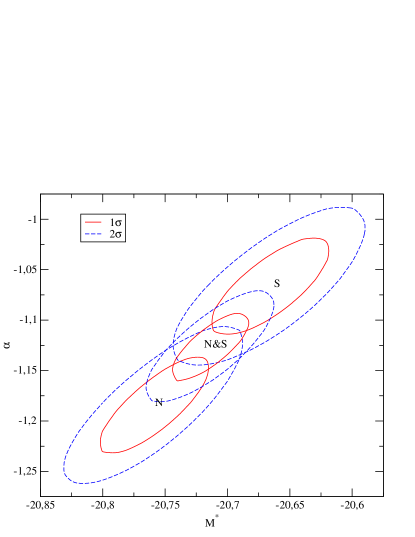
Figure 1: $1\sigma$ and $2\sigma$ error ellipses for the SDSS Northern, Southern and total samples.

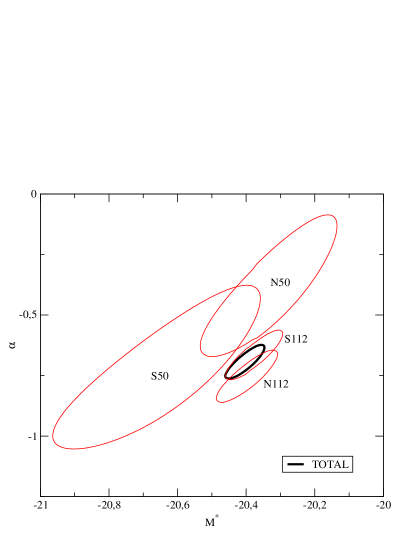
Figure 2: $1\sigma$ and $2\sigma$ error ellipses for the LCRS N50, S50, N112, S112 and total samples.

The results for the STY79 maximum likelihood method are given in Tables 1 and 2 and in Figures 1 and 2 for the SDSS and LCRS samples, respectively. Slices that are located in the Northern and Southern Galactic hemispheres are denoted by N and S, and for the LCRS the numbers 50 and 112 denote the number of fibres used. For the LCRS this kind of division is the same as used by L96 and so their Figure 4 (which was obtained assuming critical matter density) can be compared directly to Figure 2 (which assumes $\Omega_{m}=0.3,\ \Omega_{\Lambda}=0.7$). As already mentioned, luminosity function normalisation $\phi^{*}$ was calculated only for the SDSS data, giving us the value $\phi^{*}=\left(151\pm 6\right)\cdot 10^{-4}\ h^{3}$ Mpc${}^{-3}.$ If the analysis was performed separately for the Northern (N) and Southern (S) slices, then the values $0.0140\ h^{3}$ Mpc^-3 and $0.0158\ h^{3}$ Mpc^-3 were obtained for N and S, respectively. If we assumed the best values for $M^{*}$ and $\alpha$ obtained for the whole sample (i.e. $M^{*}=-20.71,\ \alpha=-1.12$) then normalisations for N and S were $0.0152\ h^{3}$ Mpc^-3 and $0.0149\ h^{3}$ Mpc^-3, respectively. Our results for $\alpha$ and $\phi^{*}$ for the SDSS N slice (which covers the commissioning phase data analysed by B01) agree well with the values quoted by B01, although for the Schechter parameter $M^{*}$ our value $-20.76$ is somewhat lower, agreeing only marginally with their result.

In Figure 3 we compare the best fitting Schechter function obtained via STY79 method with the results of the simple ’$1/V_{\max}$ method’ along with the corresponding Poissonian error-bars. This serves just as an independent cross-check of our results, although it is of course well known that ’$1/V_{\max}$ method’ gives unbiased results only for a homogeneous distribution (Felten f76 (1976)).

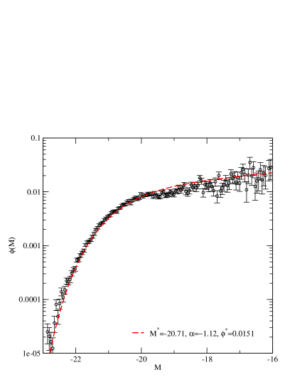
Figure 3: Results of the ’$1/V_{\max}$ method’ for the total SDSS sample with the corresponding Poissonian error-bars. The best fitting Schechter function obtained via STY79 maximum likelihood method is also given by a dashed line.

Table 1: Best fitting $M^{*}$ and $\alpha$ for the SDSS samples

Sample	$M^{*}-5\log h$	$\alpha$
N	$-\left(20.76\pm 0.04\right)$	$-\left(1.19\pm 0.05\right)$
S	$-\left(20.67\pm 0.05\right)$	$-\left(1.07\pm 0.05\right)$
TOTAL	$-\left(20.71\pm 0.03\right)$	$-\left(1.12\pm 0.03\right)$

Table 2: Best fitting $M^{*}$ and $\alpha$ for the LCRS samples

Sample	$M^{*}-5\log h$	$\alpha$
N50	$-\left(20.33\pm 0.12\right)$	$-\left(0.40\pm 0.18\right)$
S50	$-\left(20.64\pm 0.18\right)$	$-\left(0.74\pm 0.21\right)$
N112	$-\left(20.40\pm 0.05\right)$	$-\left(0.76\pm 0.07\right)$
S112	$-\left(20.40\pm 0.05\right)$	$-\left(0.70\pm 0.07\right)$
NS112	$-\left(20.38\pm 0.04\right)$	$-\left(0.70\pm 0.04\right)$
TOTAL	$-\left(20.40\pm 0.03\right)$	$-\left(0.69\pm 0.04\right)$

4 Density field

We have extracted from the SDSS and LCRS catalogues subsamples of galaxies with redshifts $z\leq 0.2$. The calculation of the density fields consists of three steps: 1) calculation of the distance, absolute magnitude, and weight factor for each galaxy of the sample; 2) calculation of rectangular coordinates of galaxies and rotation of coordinate axes in order to minimise projection effects; and 3) smoothing of the density field using an appropriate kernel and smoothing length.

Observed redshifts were first corrected for the motion relative to the CMB dipole (Lineweaver et al. lts96 (1996)). Co-moving distances of galaxies were calculated as follows (e.g. Peacock p99 (1999)):

$$r(z)=\frac{c}{H_{0}}\int\limits_{0}^{z}\left\{1+\Omega_{m}\left[\left(1+x\right)^{3}-1\right]\right\}^{-\frac{1}{2}}dx.$$ (13)

As already mentioned, we used a cosmological model with density parameters: matter density $\Omega_{m}=0.3$, dark energy density $\Omega_{\Lambda}=0.7$, total density $\Omega_{0}=\Omega_{m}+\Omega_{\Lambda}=1.0$, all in units of the critical cosmological density. With these parameters the limiting redshift $z_{lim}=0.2$ corresponds to co-moving distance $r_{lim}=571$ $h^{-1}$ Mpc. Because both surveys cover relatively thin slices on sky, we shall calculate in the following 2-dimensional density fields, projecting all galaxies to a plane through the slice. A 2-dimensional density field of SDSS EDR was calculated also by Hoyle et al. (h02 (2002)), who compared the geometry of the large-scale matter distribution with $\Lambda$CDM simulations.

Our redshift surveys cover a fixed interval in apparent magnitude which corresponds to a certain range in luminosity, $L_{1}$ and $L_{2}$, depending on the distance of the galaxy. This range, and the observed luminosity of the galaxy, $L_{obs}$, were found as described in the previous section.

We regard every galaxy as a visible member of a density enhancement (group or cluster) within the magnitude window of the group. Further we suppose that the luminosity function, calculated for the whole sample, can be applied also for individual groups and clusters. We shall discuss in Paper II problems associated with the calculation of the density field and properties of clusters and superclusters, found from density field. Based on these assumptions we calculate the number and luminosity density fields. In case of the number density the weighting factor is proportional to the inverse of the selection function,

$$w\equiv\frac{1}{n^{\mathrm{exp}}(f,D)},$$ (14)

where $n^{\mathrm{exp}}(f,D)$ is the expected number of galaxies in the whole luminosity range

$$n^{\mathrm{exp}}(f,D)=F{\frac{\int_{0}^{\infty}\phi(L)dL}{\int_{L_{1}}^{L_{2}}\phi(L)dL}}.$$ (15)

Here $F$ is the field-to-field sampling fraction, $\phi(L)$ is the luminosity function, and luminosities $L_{1}$ and $L_{2}$ correspond to the observational window of apparent magnitudes at the distance of the galaxy. The fraction $F$ takes into account the difference between 50-fibre and 112-fibre data and other effects, for details see L96. We assume that galaxy luminosities are distributed according to the Schechter function (Schechter Schechter76 (1976)):

$$\phi(L)\propto(L/L^{*})^{\alpha}\exp{(-L/L^{*})}d(L/L^{*}),$$ (16)

where $\alpha$ and $L^{*}$ are parameters. The values of these parameters used in our calculations are given in Table 3 for each of the slices. For the LCRS $-6^{\circ}$ N slice we have taken different values for $\alpha$ and $L^{*}$ since this slice was covered entirely with 50-fibre measurements.

In the case of luminous density every galaxy represents a luminosity

$$L_{tot}=L_{obs}W_{L},$$ (17)

where $L_{obs}=L_{\odot}10^{0.4\times(M_{\odot}-M)}$ is the luminosity of the visible galaxy of absolute magnitude $M$, $M_{\odot}$ is the absolute magnitude of the Sun in an appropriate filter. In the SDSS $r^{*}$ filter $M_{\odot}=4.62$ (B01) and in the Kron-Cousins R-band $M_{\odot}=4.47$ (Binney & Merrifield bm98 (1998)). The weight (the ratio of the expected total luminosity to the expected luminosity in the visibility window) is

$$W_{L}={\frac{\int_{0}^{\infty}L\phi(L)dL}{\int_{L_{1}}^{L_{2}}L\phi(L)dL}}.$$ (18)

We calculated expected luminosities by numerical integration using a finite total luminosity interval, low limit $L_{0}$ corresponds to absolute magnitude $M_{0}=-13.0$, and upper limit $L_{lim}$ to magnitude $M_{lim}=-24.5$. In the case of SDSS we adopt the apparent magnitude window $m_{1}=17.70$, $m_{2}=13.0$ in $r^{*}$-band; in the case of LCRS the apparent magnitude window is different for various fields and is taken into account using corresponding tables.

This weighting procedure was used also by Tucker et al. (Tucker00 (2000)) in the calculation of total luminosities of groups of galaxies. A different procedure was applied by Moore, Frenk & White (moore93 (1993)) (adding the expected luminosity of faint galaxies outside the observational window). We assume that density and luminosity distributions are independent, which leads to a multiplicative correction.

Table 3: Data on SDSS and LCRS slices

Sample	$\delta$	$\left\langle R.A.\right\rangle$	$\Delta\delta$	$\Delta R.A.$	$\alpha$	$M^{*}$	$N_{gal}$
SDSS	$0^{\circ}$N	$190.25^{\circ}$	$2.5^{\circ}$	$90.5^{\circ}$	$-1.12$	$-20.71$	$15221$
SDSS	$0^{\circ}$S	$23.25^{\circ}$	$2.5^{\circ}$	$65.5^{\circ}$	$-1.12$	$-20.71$	$11864$
LCRS	$-3^{\circ}$N	$191.4^{\circ}$	$1.5^{\circ}$	$81.0^{\circ}$	$-0.69$	$-20.40$	$3726$
LCRS	$-6^{\circ}$N	$189.8^{\circ}$	$1.5^{\circ}$	$77.9^{\circ}$	$-0.40$	$-20.33$	$2132$
LCRS	$-12^{\circ}$N	$191.4^{\circ}$	$1.5^{\circ}$	$81.1^{\circ}$	$-0.69$	$-20.40$	$3961$
LCRS	$-39^{\circ}$S	$12.1^{\circ}$	$1.5^{\circ}$	$113.8^{\circ}$	$-0.69$	$-20.40$	$3390$
LCRS	$-42^{\circ}$S	$12.2^{\circ}$	$1.5^{\circ}$	$112.5^{\circ}$	$-0.69$	$-20.40$	$3610$
LCRS	$-45^{\circ}$S	$12.3^{\circ}$	$1.5^{\circ}$	$114.1^{\circ}$	$-0.69$	$-20.40$	$3289$

To find the number and luminosity density fields we calculated for all galaxies rectangular equatorial coordinates as follows:

$$x = r(z_{c})\cos\delta\cos\alpha,$$

$$y = r(z_{c})\cos\delta\sin\alpha,$$ (19)

$$z = r(z_{c})\sin\delta,$$

here $z_{c}$ is the redshift, corrected for the motion relative to CMB dipole. Next we rotated this coordinate system around the $z$-axis to obtain a situation where the new $y$-axis were oriented toward the average right ascension of each slice (see Table 3) and finally we rotated this new system around its $x$-axis so as to force the average $z$-coordinate to be zero in order to minimise projection effects.

In Table 3 we also present some of the characteristic parameters for each of the studied slice as the average declination $\left\langle\delta\right\rangle$ and right ascension $\left\langle R.A.\right\rangle$, the number of galaxies, $N_{gal}$, included in the calculations of the density fields etc.

The EDR of SDSS and LCRS consists of essentially 2-dimensional slices of about $80^{\circ}$ wide and about 450 $h^{-1}$ Mpc depth. The width of slices is $1.5-2.5^{\circ}$, thus in space slices form thin conical (wedge-like) volumes; the thickness of the cones at a characteristic distance 300  $h^{-1}$ Mpc from the observer is only $8-12$ $h^{-1}$ Mpc. Due to the thin shape of slices we shall calculate only a 2-dimensional density fields.

Figure 4: Density fields of the SDSS EDR Southern slice, smoothed with $\sigma=0.8$ $h^{-1}$ Mpc dispersion. Densities are expressed in units of the mean density. Upper panel shows the number density field, lower panel the luminosity density field.

To smooth the density field two approaches are often used. The first one uses top-hat smoothing as customary in N-body calculations. In this case the density in grid corners is found by linear interpolation where the ’mass’ of the particle is divided between grid corners according to the distance from the respective corner. Variable smoothing length can be obtained by changing the size of the grid cell. A better and smoother density field can be obtained when we use Gaussian smoothing. In this case the ’mass’ of the particle is distributed between neighbouring cells using the Gaussian smoothing

$$W_{jg}=\left(2\pi\sigma_{\mathrm{sm}}^{2}\right)^{-\frac{1}{2}}\ \exp\left(-\frac{|\mathbf{x}_{j}-\mathbf{x_{g}}|^{2}}{2\sigma_{\mathrm{sm}}^{2}}\right),$$ (20)

here $\mathbf{x}_{j}$ and $\mathbf{x_{g}}$ are positions of the galaxy and the grid cell, respectively, and $\sigma_{\mathrm{sm}}$ is the smoothing length.

To calculate the density fields, we have formed a grid of cell size 1 $h^{-1}$ Mpc. On farther part of the survey only very bright galaxies can be observed, the weight factor becomes large and the fields are noisy. To decrease this effect we have calculated the density fields for the LCRS only for co-moving distance up to $r_{lim}\leq 450$ $h^{-1}$ Mpc. Very close to the observer the density fields are also noisy. Here slices become very thin in real space, and only galaxies of low luminosity fall into the window of apparent magnitudes observed. For nearby region the density fields were calculated but density enhancements were not considered as clusters if $r\leq 50$ $h^{-1}$ Mpc.

In calculations we have used several smoothing lengths. First, we tried a smoothing length $\sigma_{\mathrm{sm}}=2$ $h^{-1}$ Mpc. This smoothing yields a very smooth field where density enhancements (clusters and groups of galaxies) can be easily identified. However, the size of these enhancements clearly exceeds the size of real clusters of galaxies. Thus we have used a smaller smoothing length, $\sigma_{\mathrm{sm}}=0.8$ $h^{-1}$  Mpc, to calculate a density field which can be considered as an approximation to the true density field of dark matter associated with luminous galaxies.

To identify superclusters of galaxies we have used a larger smoothing length, $\sigma_{\mathrm{sm}}=10$ $h^{-1}$ Mpc. Experience with numerical simulations has shown that this smoothing length is suitable to select supercluster-size density enhancements (Frisch et al. f95 (1995)). To take into account the thickness of the slice, the smoothed density fields were divided by the volume of the column at the location of the particular cell in the real 3-D space, covered by observations of the slice. In this way the density fields are reduced to a plane parallel sheet of constant thickness.

The high-resolution number and luminosity density fields for the SDSS EDR Southern slice are shown in Figure 4. The density fields of all EDR SDSS slices are presented in Einasto et al. (e02a (2002)), the fields of LCRS slices are presented in Einasto et al. (e02b (2003)).

5 Analysis

So far we have determined the number and luminosity density fields for the SDSS EDR and LCRS samples. In order to estimate the selection effects we have calculated the luminosity function assuming Schechter type of parametrisation.

To be sure that we are not grossly under- or overestimating the statistical weights we are applying to visible objects (in order to take account their invisible companions), we perform some simple calculations. Namely, we calculate the number and luminosity density averaged over thin shells as a function of the coordinate distance. What concerns the number density, then we expect it to fall in the distant part of the samples since there we miss some of the faintest systems totally. The same need not be true for the luminosity density since even the modest amount of luminosity evolution could compensate the decrease in the number density. The results for the number and luminosity density for the SDSS EDR data are given in Figure 5. We see that indeed the number density starts to decline at the largest distances, as expected, indicating that we are at the right track. Contrary to the number density the luminosity density is almost constant for the Northern slice, but shows a slightly increasing trend in the Southern slice on large distances. This is also evident from the Figure 4 where densities are colour coded. For the LCRS slices we get essentially the same results and for the brevity we are not going to present them here. All this suggests that our statistical weighting scheme looks quite reasonable for such a preliminary study.

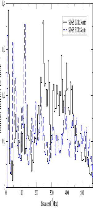
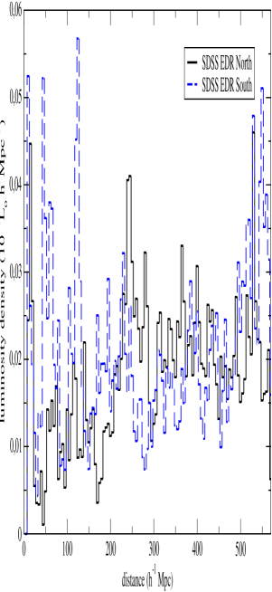
Figure 5: Upper and lower panels show respectively the number and luminosity density as a function of coordinate distance for the SDSS Northern and Southern slices using the best fitting Schechter parameters for the total sample as given in Table 1. Densities were calculated using the high-resolution field.

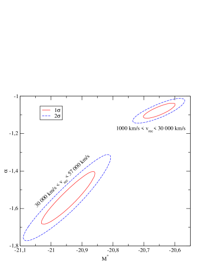
Figure 6: $1\sigma$ and $2\sigma$ error ellipses for the SDSS data divided into low $z$ and high $z$ subsamples.

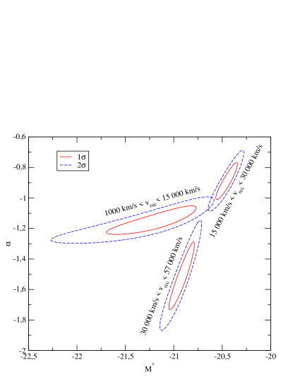
Figure 7: $1\sigma$ and $2\sigma$ error ellipses for the SDSS EDR Southern slice data divided into three $z$ intervals.

The second thing we want to mention is the fact that we have assumed that the same Schechter parameters $M^{*}$ and $\alpha$ apply for the whole sample. In order to study the possible evolution with redshift $z$ we have divided our SDSS EDR sample into two parts: low $z$ part ($v_{rec}=1000\ldots 30000$ km/s) and high $z$ part ($v_{rec}=30000\ldots 57000$ km/s) and performed the STY79 maximum likelihood analysis for both of these separately. The results that are given in Figure 6 probably suggest that $M^{*}$ and $\alpha$ are evolving in time. From this figure we obtain a simple linear approximation

$$M^{*} = -4.2z-20.37,$$

$$\alpha = -6.7z-0.63,$$ (21)

where we have taken into account the fact that the average $z$ for the low $z$ sample is 0.067 and for the high $z$ one 0.136. If we assume this kind of $M^{*}$ and $\alpha$ dependences on $z$ for the whole sample and calculate the number and luminosity densities as above then we get pretty bad results. So certainly this kind of big linear variation with $z$ makes things worse.

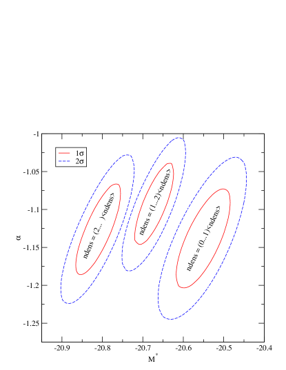
Figure 8: $1\sigma$ and $2\sigma$ error ellipses for the SDSS EDR Southern slice data divided into three global density $\delta$ intervals.

Table 4: Luminosity function parameters in different environment

Sample	$M^{*}-5\log h$	$\alpha$
$0<\delta_{0}\leq 1.0$	$-20.55\pm 0.07$	$-1.14\pm 0.06$
$1.0<\delta_{0}\leq 2.0$	$-20.67\pm 0.07$	$-1.09\pm 0.05$
$2.0<\delta_{0}$	$-20.81\pm 0.07$	$-1.13\pm 0.05$

Next we divide the SDSS EDR Southern sample into three parts: $v_{rec}=1000\ldots 15000$ km/s, $v_{rec}=15000\ldots 30000$ km/s and $v_{rec}=30000\ldots 60000$ km/s. In this case we get non-monotonic dependences for $M^{*}$ and $\alpha$ on $z$ (see Figure 7). We also notice that variations in $M^{*}$ and $\alpha$ are correlated with the density of the surroundings: due to the effects of the nearby dense regions the value for $M^{*}$ is smaller than on average; as we move further away $M^{*}$ gets bigger, which is caused by the large void at distances $\sim 200\ldots 350\ h^{-1}$ Mpc (see Figure 4). In distant parts, as the density rises again, $M^{*}$ gets accordingly smaller. This suggests that environmental effects are more important than evolutionary ones (which we expect to be monotonic in $z$), and so the usual assumption in determining the luminosity function $\phi\left(M\right)$ that it is independent of the spatial position cannot be strictly correct.

Figure 9: Luminosities of Southern slice galaxies as a function of the global relative density $\delta$ smoothed with 2 $h^{-1}$ Mpc dispersion. Luminosities are expressed in units of $10^{10}$ Solar luminosities, global density $\varrho$ in units of the mean density. The Northern slice has similar dependence on the environmental density.

To study this aspect in more detail we calculated the dependence of luminosity function parameters on the density of the environment. We calculated for every galaxy the global density $\delta_{0}$ (with 10 $h^{-1}$ Mpc smoothing) and used this value as environmental parameter. Galaxies were divided into three types according to density (expressed in units of the mean density). Parameters of the luminosity function are given in Table 4 and Figure 8. We see that parameter $M^{*}$ changes considerably with density: in high-density regions its value is more negative, i.e. galaxies are brighter. A similar tendency has been recently observed in other surveys (Bromley et al. (1998), Beisbart & Kerscher (2000), Norberg et al. (2001)).

The density field with 10 $h^{-1}$ Mpc smoothing characterizes the density on supercluster scales. The dependence of galaxy luminosity on density has been found also on smaller scales. In Figure 9 we plot luminosities of galaxies of the Southern SDSS EDR slice as a function of the density smoothed on 2 $h^{-1}$ Mpc scale. This smoothing is sensitive to density changes within clusters of galaxies and in galaxy filaments. We see a strong dependence of the upper end of luminosities: brightest galaxies in low-density regions are about 5 times less luminous than in high-density regions. This difference in luminosity corresponds to a difference 1.7 magnitudes, much more than expected from the analysis based on larger smoothing length. We plan to address all these issues in more detail in the forthcoming papers. Physical interpretation of these phenomena needs theoretical studies.

We repeat that all the density fields (see Figure 4) compiled in this paper refer to the redshift space.

6 Conclusions

In this paper we have calculated the galaxy luminosity function for the SDSS EDR and LCRS samples and used it to construct the number and luminosity density fields (smoothed on $0.8\ h^{-1}$ Mpc scale) assuming flat underlying cosmologies with $\Omega_{m}=0.3$ and $\Omega_{\Lambda}=0.7.$ The analysis presented here is rather simple and serves as a first step in the study of the distribution of galaxies in SDSS and LCRS samples. The principal conclusion from our study is: parameters of the galaxy luminosity function depend on the distance from the observer, density of the environment, they are different for the Northern and Southern slice. The largest effect is the dependence on the density of the environment: in high-density regions brightest galaxies are more luminous than in low-density regions by a factor up to 5 (1.7 magnitudes). Some of these effects suggest that it is not yet possible to find an universal set of parameters of the luminosity function valid for a fair sample of the Universe. In other words, presently available samples are still too small to be considered as candidates for the fair sample.

References

- (1) Basilakos, S., Plionis, M., & Rowan-Robinson, M., 2001, MNRAS, 323, 47
- Beisbart & Kerscher (2000) Beisbart, C. & Kerscher, M., 2000, ApJ, 545, 6
- (3) Binney, J., & Merrifield, M., 1998, Galactic Astronomy (Princeton: Princeton University Press)
- (4) Blanton, M.R., Dalcanton, J., Eisenstein, D. et al., 2001, AJ, 121, 2358 (B01)
- Bromley et al. (1998) Bromley, B. C., Press, W. H., Lin, H. & Kirshner, R. P., ApJ, 505, 25
- (6) Einasto, J., Hütsi, G., Einasto, M., Saar, E., Tucker, D. L., Müller, V., Heinämäki, P., & Allam, S. S., 2002, A&A, (submitted) (Paper II)
- (7) Einasto, J., Einasto, M., Hütsi, G., Saar, E., Tucker, D. L., Jaaniste, J., Müller, V., Heinämäki, P., & Allam, S. S., 2003, A&A, (in preparation) (Paper III)
- (8) Efstathiou, G., Ellis, R.S., & Peterson, B.A., 1988, MNRAS, 232, 431
- (9) Felten, J.E., 1976, ApJ, 207, 700
- (10) Frisch, P., Einasto, J., Einasto, M., Freudling, W., Fricke, K. J., Gramann, M., Saar, V. & Toomet, O., 1995, A&A, 296, 611
- Goto et al. (2002) Goto T., Okamura S., McKay T. A., et al., 2002, PASJ, 54, 515
- (12) Gott, J.R., Melott, A.L., & Dickinson, M., 1986, ApJ, 306, 341
- (13) Hoyle, F., Vogeley, M.S., Gott, J.R. et al., 2002, MNRAS (submitted), astro-ph/0206146
- (14) Lin, H., Kirshner, R.P., Shectman, S.A., Landy, S.D., Oemler, A., Tucker, D.L., & Schechter, P.L., 1996, ApJ, 464, 60 (L96)
- (15) Lineweaver, C.H., Tenorio, L., Smoot, G.F., Keegstra, P., Banday, A.J., & Lubin, P., 1996, ApJ, 470, 38
- (16) Lynden-Bell, D., 1971, MNRAS, 155, 95
- (17) Moore, B., Frenk, C. S. & White, S.D.M., 1993, MNRAS, 261, 827
- Norberg et al. (2001) Norberg, P., Baugh, C.M., Hawkins, E. et al. (2001), MNRAS, 328, 64
- (19) Peacock, J.A., 1999, Cosmological Physics (Cambridge: Cambridge University Press)
- (20) Press, W.H., Teukolsky, S.A., Vetterling, W.T., & Flannery, B.P., 1992, Numerical Recipes (Cambridge: Cambridge University Press)
- (21) Sandage, A., Tammann, G.A., & Yahil, A., 1979, ApJ, 232, 352 (STY79)
- (22) Saunders, W., Frenk, C., Rowan-Robinson, M., Lawrence, A., & Efstathiou, G., 1991, Nature, 349, 32
- (23) Saunders, W., Sutherland, W. J., Maddox, S. J. et al., 2000, MNRAS, 317, 55
- (24) Schechter, P., 1976, ApJ, 203, 297
- (25) Schmidt, M., 1968, ApJ, 151, 393
- (26) Schlegel, D.J., Finkbeiner, D.P., & Davis, M., 1998, ApJ, 500, 525
- (27) Shectman, S.A., Landy, S.D., Oemler, A., Tucker, D.L., Lin, H., Kirshner, R.P., & Schechter, P. L., 1996, ApJ , 470, 172
-
(28)
Shimasaku, K.,
http://www.astron.s.u-tokyo.ac.jp/~shima/
sed.tar.Z - (29) Stoughton, C., Lupton, R. H., Bernardi, M. et al., 2002, AJ, 123, 485
- (30) Tucker, D.L., 1994, Ph.D. Thesis, Yale University
- (31) Tucker, D.L., Oemler, A.Jr., Hashimoto, Y., Shectman, A., Kirshner, R.P., Lin, H., Landy, S.D., Schechter, P.L., & Allam, S.S., 2000, ApJS, 130, 237