Cosmic Shear with Next Generation Redshift Surveys as a Cosmological Probe

Abstract

The expansion of the universe causes spacetime curvature, distinguishing between distances measured along and transverse to the line of sight. The ratio of these distances, e.g. the cosmic shear distortion of a sphere defined by observations of large scale structure as suggested by Alcock & Paczyński, provides a method for exploring the expansion as a function of redshift. The theoretical sensitivity to cosmological parameters, including the dark energy equation of state, is presented. Remarkably, sensitivity to the time variation of the dark energy equation of state is best achieved by observations at redshifts $z\mathrel{\mathchoice{\lower 3.6pt\vbox{\halign{$\mathsurround=0pt\displaystyle\hfil#\hfil$\cr<\crcr\sim\crcr}}}{\lower 3.6pt\vbox{\halign{$\mathsurround=0pt\textstyle\hfil#\hfil$\cr<\crcr\sim\crcr}}}{\lower 3.6pt\vbox{\halign{$\mathsurround=0pt\scriptstyle\hfil#\hfil$\cr<\crcr\sim\crcr}}}{\lower 3.6pt\vbox{\halign{$\mathsurround=0pt\scriptscriptstyle\hfil#\hfil$\cr<\crcr\sim\crcr}}}}1$. While systematic errors greatly degrade the theoretical sensitivity, this probe may still offer useful parameter estimation, especially in complementarity with a distance measure like the Type Ia supernova method implemented by SNAP. Possible future observations of the Alcock-Paczyński distortion by the KAOS project on a 8 meter ground based telescope are considered.

I Introduction

We now have strong evidence that the expansion of the universe is accelerating, from the original method of Type Ia supernova distance-redshift measurements perl99 ; riess98 and concordant observations of the cosmic microwave background (CMB) power spectrum and of large scale structure bond ; perc . Understanding the nature of the dark energy responsible for the acceleration will have profound implications for cosmology, high energy physics, and fundamental physics. Mapping the expansion history of the universe offers a way to gain insights into the dark energy and the fate of the universe, for example by characterizing the equation of state behavior which is directly related to properties of the scalar field potential.

Distance measures, notably the supernova method, have proved useful at constraining the energy density and equation of state of the dark energy, with great improvements expected in the next decade. But these involve an integration over the expansion rate behavior $H(z)$, which itself involves a redshift integral over the equation of state $w(z)$. We can ask whether we can devise a more direct probe of the acceleration. In fact one such, the redshift drift test, was proposed by Sandage san61 in 1961 and developed further by Linder lin97 .

The redshift of a source is a central astrophysical observable. It is directly related to the change in time intervals due to the cosmic expansion between a photon’s emission and observation, $z=dt_{o}/dt_{e}-1=a_{o}/a_{e}-1$, where $a(t)$ is the scale factor of the universe. But obviously one could consider a second derivative term, a time dependence of the redshift itself as the universe ages:

$${dz\over dt_{o}} = {d\over dt_{o}}\left[{a(t_{o})\over a(t_{e})}\right]=[\dot{a}(t_{o})-\dot{a}(t_{e})]/a(t_{e})$$ (1)

$$= H_{0}(1+z)-H(z).$$ (2)

This provides a direct measure of acceleration, being effectively a second time derivative, as can be seen from the low redshift limit: $\Delta z/z\approx-q_{0}H_{0}\Delta t$, where $q_{0}$ is the present deceleration parameter. However since the astronomical observing time is much smaller than the Hubble time, $\Delta t\ll H_{0}^{-1}$, this is not a practical probe. For example in the most optimistic case of observing over a period of 10 years a hypothetical spectral line emitted at the CMB last scattering surface at $z=10^{3}$, one requires a redshift measurement of a part in $10^{5}$ to distinguish cosmological models. For emission line objects at $z=5$, this becomes a part in $10^{8}$.

Moreover, just as peculiar velocities affect redshift measurements at the level of $v/c$, so do peculiar accelerations, i.e. local gravitational potentials $\Phi$ from inhomogeneously distributed matter, affect the redshift drift measurements at a level $\Phi/c^{2}\approx 10^{-5}$. This latter effect even ruins the generalization of the redshift drift called the cosmic pulsar test, where timing is improved by measuring a large number $N$ of wavelengths or pulses lin97 .

But if we are stymied in measuring the acceleration directly, at least we can hope to measure the first derivative of the expansion, $H(z)$. One of the ways to do this is the cosmic shear, or Alcock-Paczyński  test. Section II sets up the formalism while Section III applies Fisher matrix analysis to investigate the theoretical sensitivity of this method for estimating the cosmological parameters. In Section IV we introduce observational sanity in the form of systematic uncertainties and discuss the proposed KAOS project as a means of carrying out this test. We summarize our conclusions and plans for future work in Section V.

II Cosmic Shear Test

Proper distances measured along the line of sight carry information through light emitted at different times in the expansion history of the universe. Therefore in a sphere of comoving points, differences in the emission times lead to probing the geometry at different expansion rates. So observationally a sphere will appear to be distorted, or sheared, with the magnitude of the effect sensitive to the expansion rate. This is the cosmic shear effect discussed by Alcock & Paczyński (ap ; do not confuse this with shear from weak gravitational lensing – due to inhomogeneities rather than the global structure of spacetime).

In more detail, if we consider the small difference in radial distance between nearby emitters, then we localize the behavior in redshift and essentially measure the expansion rate at that time. However transverse to the radial direction the angular separation between comoving points is measured at a constant value of the scale factor $a(t_{e})$, and then the light from each source propagates over the same intervening distance to the observer at $t_{o}$. Thus in the radial case the data gives a snapshot of the expansion rate while the transverse distance contains an integration over the expansion history from emission to observation.

Consider a sphere of comoving points. The distance through the center of the sphere along the line of sight is the proper distance,

$$dr_{\parallel}=dt=a(t)\,dr_{c}=(1+z)^{-1}H^{-1}(z)\,\Delta z.$$ (3)

The transverse distance is

$$dr_{\perp}=r_{a}(z)\,\Delta\theta=(1+z)^{-1}r_{c}(z)\,\Delta\theta,$$ (4)

where $z=a^{-1}-1$ is the redshift, $H=\dot{a}/a$ is the Hubble parameter, $r_{c}$ the comoving distance, and $r_{a}$ the angular distance (see, for example, lin97 ).

From the observables of the angular scale $\Delta\theta$ of such comoving sources, their central redshift $z$, and their redshift extent $\Delta z$, one can form a quantity

$$D(z)\equiv\Delta z/\Delta\theta=H(z)\int_{0}^{z}dz^{\prime}/H(z^{\prime}).$$ (5)

The cosmic shear is then

$$S=\sqrt{2\left[1-\left({\Delta z\over\Delta\theta}\right)^{2}\right]}.$$ (6)

This has some excellent properties for a cosmological probe. In particular, it has dependence on $H(z)$ directly, not just through an integral. Since $H$ is related to the energy density of the universe then one can try to map the density history and equation of state. Indeed for time varying equation of state of the dark energy $w(z)$, $H$ depends on an integral of $w(z)$, so distance measures involve $w(z)$ as a double integral. Therefore one might hope that the Alcock-Paczyński differential distance test might be more sensitive to reconstructing the dark energy equation of state than a standard distance test.

Another interesting characteristic of (5) is that it does not depend on any absolute scale, since $H$ appears in both numerator and denominator. So there is no absolute measurement to marginalize over.

The physics of the test seems clean, using pure geometry of the background spacetime, so long as we can find sources that are comoving and defining a known local spatial geometry. Conventionally the local source geometry is taken to be spherical, as it would be for an isotropic arrangement. Possibilities for defining isotropically arranged sources include large coherent objects such as superclusters in the linear density regime and so following the isotropic expansion of the universe, or lengths defined through correlation functions between individual objects, such as for galaxies or Lyman alpha forest absorbers. The extent to which these assumptions break down or cannot be corrected yield systematic errors to plague the method. As for many other cosmological probes, the systematic errors turn out to be more severe than statistical errors from insufficient data. Section IV discusses this further.

III Sensitivity to Cosmological Parameters

We begin by considering a purely theoretical analysis of the capabilities of the test, leaving observational realities for §IV. A good way to understand the sensitivities and degeneracies of cosmological probes is through Fisher matrix analysis of the dependence of the observable on the parameters. We take a flat universe defined by three parameters: the dimensionless matter density $\Omega_{m}$ (so the dark energy density is $1-\Omega_{m}$), the value of the dark energy equation of state today $w_{0}$, and a measure of its time variation $w^{\prime}$. Since we want to consider observations extending to redshifts greater than unity, e.g. Lyman alpha observations are most plentiful with $z\approx 3$, we adopt the equation of state parametrization $w(z)=w_{0}+w_{a}z/(1+z)$ with the definition $w^{\prime}=dw/d\ln(1+z)|_{z=1}=w_{a}/2$ linwa . This approximates well the behavior of several classes of dark energy models, especially those with a slow roll phase, is well behaved even for $z>1$, and allows insight into the effects of the physically expected time variation in the equation of state.

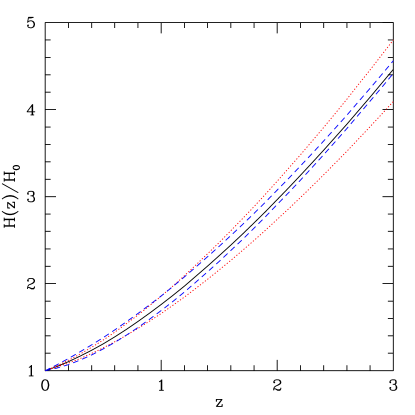
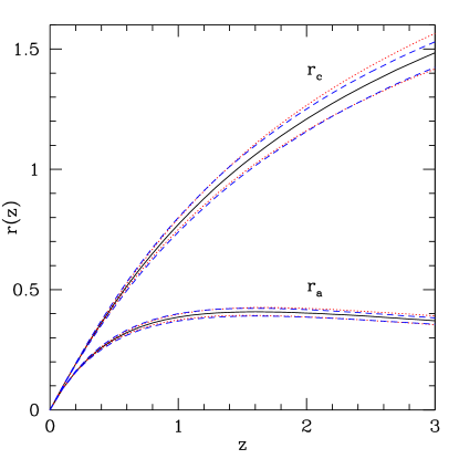
The distance distortion $D(z)=H(z)\int dz/H$ differs in its behavior in an interesting way from distance or volume measures: the two factors actually depend on the cosmological parameters in opposite ways because they have reciprocal dependence on the expansion rate. At low redshift the direct $H(z)$ dependence dominates since all distances must be similar. But at high redshifts the universe was matter dominated and so $H(z\gg 1)$ is insensitive to the equation of state parameters and the distance factor takes over, since it retains memory of those parameters due to its integral nature.

Figures 1 and 2 show the dependence of the Hubble parameter and the distances $r_{c}$ and $r_{a}$, respectively, on the cosmological parameters $\Omega_{m}$ and $w_{0}$ ($w_{a}$ behaves similarly). One clearly sees that the dependencies are in inverse relation. This implies that there can be crossover ranges in redshift where the distance distortion $D$ is essentially independent of one of the parameters. While this makes it impossible to determine that aspect of cosmology with observations in that redshift range, it has a benefit as well. From the figures one can deduce that degeneracies exist where one parameter can be adjusted to counteract the effect of another. But at the crossover points one parameter will not affect the distortion and so the degeneracy can be broken. Essentially, observations near a crossover apply to a reduced phase space, and hence the other parameter estimates will be sharper. This is clearly seen in later figures.

Figure 1: The Hubble parameter $H(z)$ as a function of redshift, for the fiducial flat model $\Omega_{m}=0.3$, $w=-1$ (solid curve) and variants. Upper (lower) dotted curves have $\Omega_{m}=0.35$ (0.25); upper (lower) dashed curves have $w=-0.8$ ($-1.2$).

Figure 2: The comoving distance $r_{c}$ and angular distance $r_{a}$ as a function of redshift, for the same models as Fig. 1. However now upper and lower models are interchanged, e.g. the upper dotted curve has $\Omega_{m}=0.25$ etc.

An excellent way to explore the sensitivity of an observational test to the cosmology is through Fisher matrix analysis tegfis . This methodology approximates the likelihood surface of the parameter fit to observations with a gaussian probability near the best fit, the fiducial model. The sensitivity of its estimation of parameter values depends on the derivatives of the observational quantity with respect to the parameter, $\partial D/\partial x$, and the precision with which the observations can be made. Writing the errors as $\delta D=(\delta D/D)D$, we see that for a given fractional measurement precision $\sigma_{D}\equiv\delta D/D$ we can obtain a parameter error estimate $\delta x$ by investigating $\partial\ln D/\partial x$. Figure 3 shows this central quantity of Fisher analysis.

Figure 3: The sensitivity of the observable, here $D=H(z)\,r_{c}(z)$, to the cosmological parameters is encoded in the derivatives plotted here. The larger the absolute magnitude of the derivative at a particular redshift, the more constraining the observations there.

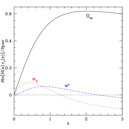
Indeed we can read off almost all of our results from this sensitivity graph. The previously discussed crossovers are clear, with the probe aloof to $w_{0}$ around $z\approx 1.3$ and to $w^{\prime}$ (i.e. $w_{a}$) around $z\approx 2.3$. Sensitivity to $\Omega_{m}$ grows out to $z\approx 1$, after which it levels off; $w_{0}$ has a sweet spot at $z\approx 0.4$ and again above $z\approx 2$; the time variation $w^{\prime}$ has a broad, though low, impact from $z\approx 0.6-1.1$. However at $z\approx 1.3$ we expect $w^{\prime}$ to be uncorrelated with $w_{0}$ and so possibly easier to determine.

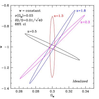
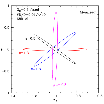
Also note that while at low redshift the sensitivities to $\Omega_{m}$ and $w_{0}$ enter with the same sign, this changes after the $w_{0}$ crossover. This means that at low redshift the error ellipse in the $w_{0}-\Omega_{m}$ plane will have the same orientation as for the supernova distance case: making $w_{0}$ larger (less negative) can be counteracted by making $\Omega_{m}$ smaller, defining a degeneracy direction in that plane. However higher redshift cosmic shear observations will have an orthogonal degeneracy direction, holding out the promise of complementarity with supernovae. A similar rotation of error ellipse contours with redshift can be predicted between $w_{0}$ and $w^{\prime}$.

Figure 3 for the Fisher sensitivity even allows us to calculate lower limits on the precision with which we can estimate the parameters:

$$\delta x>(\partial\ln D/\partial x)^{-1}\sigma_{D}.$$ (7)

This lower limit refers to fixing all parameters but one, and so will underestimate the true error due to degeneracies. If we take, say, 1% precision in observations, then the lower limits on estimating $\{\Omega_{m},w_{0},w^{\prime}\}$ are 0.015, 0.1, 0.15 for the peaks of the sensitivity curves. However multiple observations can improve on the precision, while systematic errors will put a floor on it. To proceed further quantitatively we must input an observational suite into the Fisher method.

To best illustrate the results we begin with a simple set of observations. We assume equal numbers $n$ of observations in redshift bins of width 0.1, each with the same precision $\sigma_{D}$, and vary the redshift range the observations cover. Initially we apply only statistical errors and so only the combination $\sigma_{D}/\sqrt{n}$ matters.

Purely to test our intuition from the Fisher sensitivity figure, we take the highly idealized situation of constant $w(z)$ (i.e. fix $w^{\prime}=0$ a priori) in Figure 4 and fixed $\Omega_{m}$ in Figure 5, as well as unrealistically good precision. The rotation of the contours with redshift is clear. Note that for the crossover redshift $z\approx 1.3$ the determination of $w_{0}$ is uncorrelated with the other parameters, i.e. the contours are vertical or horizontal.

Figure 4: Idealized results for estimation of $w$ and $\Omega_{m}$, with only statistical errors. Note the equation of state is fixed to be constant a priori. This is purely illustrative, showing the rotation of degeneracy directions and decorrelation at the crossover redshift. The sizes of the ellipses are idealized, corresponding to pure statistics for 40 observations of precision 1% in a 0.1 bin in redshift.

Figure 5: Idealized results for estimating $w^{\prime}$ and $w_{0}$, with $\Omega_{m}$ fixed and only statistical errors. This is purely illustrative, showing the rotation of degeneracy directions and decorrelation at the crossover redshifts. The sizes of the ellipses are idealized, corresponding to pure statistics for 40 observations of precision 1% in a 0.1 bin in redshift.

IV Systematic Uncertainties and Observational Methods

Virtually all proposed observational methods for probing cosmology run into limits imposed by systematic uncertainties rather than statistical errors. So although the cosmic shear test appears rather promising in its sensitivity to parameters and complementarity with other probes, as expected from its inclusion of a bare factor $H(z)$ as discussed in the first two sections, it behooves us not to make estimates of its power merely by speculating on achievable future survey statistics. For more realistic assessment of the promise of this method for determination of cosmological parameters, we must investigate the effect of systematics. Detailed characterization of irreducible uncertainities requires a comprehensive survey design and analysis; instead we present here a simple model that should illustrate the main effects and give reasonably realistic quantitative results.

We adopt a precision of 2% in measurement, with $n=10$ observations per 0.1 redshift bin, but also include an irreducible systematics floor of 2% in a bin. This makes the actual numbers used for the statistical error moot, except when we later consider a systematic that declines at low redshifts. Generally we adopt a gaussian prior on the matter density of 0.03, but also investigated 0.01. The plots show results for observations over redshift ranges, e.g. $z=1-2$.

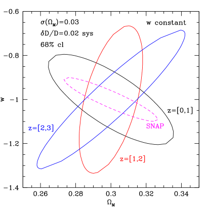
Figure 6 shows the $w-\Omega_{m}$ plane, disallowing the possibility of any time variation in the equation of state – an a priori assumption without justification. Note that systematics have a large effect on the Alcock-Paczyński test. In particular they wipe out most of the complementarity at high redshift with the supernova method that was given by the $w$ sensitivity crossover and resulting rotation of the error ellipse. (Note that the contours for the next generation supernova survey, SNAP, include systematics.) Some complementarity is retained for observations at $z>2$, allowing an improvement in determining $w$ and $\Omega_{m}$ by a factor two. Of course modeling the dark energy as a constant equation of state becomes even more suspect as one increases the range of observation.

Figure 6: Parameter estimation in the $w-\Omega_{m}$ plane, with systematics. Note the equation of state is assumed constant a priori. Contours correspond to the 68% confidence level.

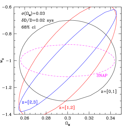
When one removes the constraint that the equation of state must be constant a priori, the Alcock-Paczyński test does not offer any improvement to SNAP in estimation of the present value of the equation of state $w_{0}$, as seen in Figure 7. The combination of the two experiments does help to limit $\Omega_{m}$, but so does, for example, the weak gravitational lensing survey that is an integral part of the SNAP mission.

Figure 7: Parameter estimation in the $w_{0}-\Omega_{m}$ plane, with systematics, marginalizing over $w^{\prime}$. Removing the prior that $w=$ constant strongly inflates the error contours.

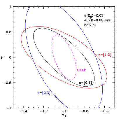
In the $w^{\prime}-w$ plane (recall $w^{\prime}\equiv w_{a}/2$), Figure 8 illustrates that not fixing $\Omega_{m}$ has a drastic effect on the error contours in comparison to the thin ellipses of Figure 5. Uncertainty in $\Omega_{m}$ broadens the contours in a more or less fixed direction in this plane, though, so it affects the ellipses for some redshift ranges less than others. For example data around $z\approx 0.7$ does not suffer as much loss of sensitivity to the equation of state parameters. Indeed observations covering the range of $z=0-1$ at 2% precision permit determination of the time variation of the equation of state with errors about 30% looser than from SNAP. Unfortunately the respective error regions mostly overlap, with little complementarity. Still, they would provide independent checks of the results using very different methods.

Figure 8: Parameter estimation in the $w^{\prime}-w_{0}$ plane, with systematics, marginalizing over $\Omega_{m}$. Realistic assessment of systematics is key to evaluating the impact of the cosmic shear test.

In a bid to optimize the parameter determination we can examine how best to concentrate the observations, and over what redshift range. Given a systematics floor, an increase in the numbers of observations within a bin or an improvement in the statistical precision accomplishes little. An exception to this would be if external systematics needed to be reduced, for example by dividing the data into subsets for a “like to like” comparison. As for the redshift range, the results found here indicate that relatively little leverage is gained, for the given prior and systematics, outside the range $z\approx 0.2-0.9$.

This is well suited for ground based observations by large telescopes within a decade. Such a cosmic shear survey could be carried out by the KAOS project: the Kilo-Aperture Optical Spectrometer proposed as a front end for the 8 meter Gemini South telescope. This would have multiplexing capability from some 4000 apertures to measure detailed velocity maps of supercluster environments. In such a linear overdensity region one might hope to apply the Alcock-Paczyński test without any complications of nonlinear gravitational physics or gas dynamics. Another possibility is studying the anisotropy of correlation functions of subclasses of bright galaxies. Both approaches can cover the preferred redshift range and statistics would not be a problem with a 1.5 square degree field of view and coverage of some 400 square degrees of sky to measure precise redshifts for $10^{6}$ galaxies.

Observations at $z>1$ were shown to be fairly insensitive to the dark energy equation of state for the cosmic shear test, and thus can be used robustly to learn about astrophysics, perhaps from Lyman alpha forest observations. Of course the rich panoply of data from such a next generation survey as KAOS can be examined with other cosmological probes as well (with similar cautions and care for the influence of systematic uncertainties).

V Conclusion

The cosmic shear test looks extremely promising theoretically for the determination of cosmological parameters. This is evident from its tomographic dependence on the expansion rate of the universe, shown by the appearance of the Hubble parameter $H(z)$ by itself. It has further interesting properties in the redshift evolution of its parameter degeneracies and complementarity with other probes.

However, systematic uncertainties, most probably involving peculiar velocities and distortions related to the local environment rather than cosmic expansion, put severe limits on the probe’s ability to fulfill its potential.

Unless systematic uncertainties can be brought under the 2% level, the cosmic shear test applied at low or high redshift does not appear to offer significantly complementary or generally comparable limits to the supernova distance method. Considering a linear systematic of $0.02z$, a matter density prior $\sigma(\Omega_{m})=0.01$, or the addition of Planck CMB data does not greatly affect these conclusions.

The best hope for applying this method does, however, lie at redshifts $z<1$, which is observationally feasible. Therefore careful study of the systematic uncertainties might yield some regime in which the next generation of wide, deep redshift surveys can bring this method of determining cosmological parameters to fruition.

References

- (1) S. Perlmutter et al., Astrophys. J. 517, 565 (1999)
- (2) A. Riess et al., Astron. J. 116, 1009 (1998)
- (3) J.R. Bond et al., in Theoretical Physics, MRST 2002: A Tribute to George Libbrandt (AIP), eds. V. Elias, R. Epp, R. Myers, astro-ph/0210007
- (4) W.J. Percival et al., to appear in MNRAS, astro-ph/0206256
- (5) A. Sandage, Ap.J. 133, 355 (1961)
-
(6)
E.V. Linder, First Principles of Cosmology
(Addison-Wesley, London, 1997), p. 54-56;
http://supernova.lbl.gov/~evlinder/umass/drift.html - (7) C. Alcock and B. Paczyński, Nature 281, 358 (1979)
- (8) Linder, E.V., submitted to Phys. Rev. Lett., astro-ph/0208512
- (9) M. Tegmark, D.J. Eisenstein, W. Hu, R. Kron, astro-ph/9805117