Mass-temperature relation of galaxy clusters: implications from the observed luminosity-temperature relation and X-ray temperature function

Abstract

We derive constraints on the mass-temperature relation of galaxy clusters from their observed luminosity-temperature relation and X-ray temperature function. Adopting the isothermal gas in hydrostatic equilibrium embedded in the universal density profile of dark matter halos, we compute the X-ray luminosity for clusters as a function of their hosting halo mass. We find that in order to reproduce the two observational statistics, the mass-temperature relation is fairly well constrained as $T_{\rm gas}=(1.5\sim 2.0)\;{\rm keV}(M_{\rm vir}/10^{14}h_{70}^{-1}M_{\odot})^{0.5\sim 0.55}$, and a simple self-similar evolution model ($T_{\rm gas}\propto M_{\rm vir}^{2/3}$) is strongly disfavored. In the cosmological model that we assume (a $\Lambda$CDM universe with $\Omega_{0}=0.3$, $\lambda_{0}=0.7$ and $h_{70}=1$), the derived mass-temperature relation suggests that the mass fluctuation amplitude $\sigma_{8}$ is 0.7–0.8.

1 Introduction

While clusters of galaxies are relatively simple dynamical systems that consist of dark matter, stars, and X-ray–emitting hot gas, their thermal evolution is not yet fully understood. This is clearly illustrated by the well-known inconsistency of the observed X-ray luminosity-temperature ($L_{\mathrm{X}}$-$T$) relation, $L_{\mathrm{X}}\propto T^{3}$ (e.g., David et al., 1993; Markevitch, 1998; Arnaud & Evrard, 1999) against the simple self-similar prediction $L_{\mathrm{X}}\propto T^{2}$ (Kaiser, 1986). Conventionally this is interpreted as evidence for preheating of intracluster gas; additional heating tends to increase the temperature and the core size of the cluster, and to decrease the central density and the luminosity. Since the effect is stronger for less massive systems, the slope of $L_{\mathrm{X}}$-$T$ relation becomes steeper than that of the self-similar prediction (Evrard & Henry, 1991; Kaiser, 1991).

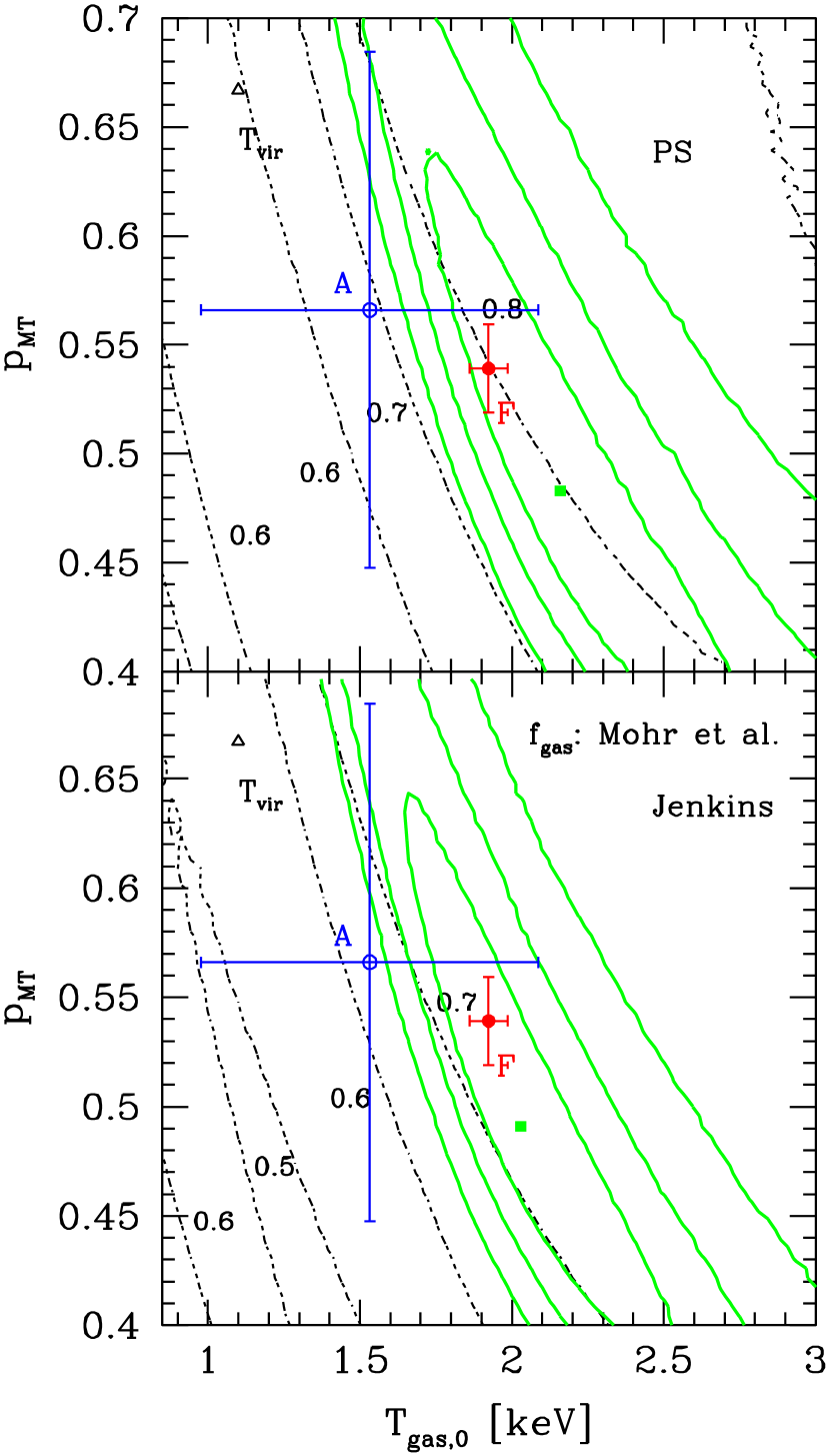
Figure 5: Constraints on the parameterized $M$-$T$ relation of clusters from the $\chi^{2}$ fit to the observed XTF. Upper and lower panels adopt the mass functions of Press & Schechter (1974) and Jenkins et al. (2001), respectively. The three solid contour curves represent the 1, 2, and $3\;\sigma$ confidence levels, with the filled squares indicating the points of the highest significance. Dotted contour curves show the best-fit values for $\sigma_{8}$ (which label each curve). Symbols are as in Fig. 3.

In addition, the mass-temperature ($M$-$T$) relation of clusters is also poorly determined. Although it is conventionally assumed that the gas shock heating is efficient enough and the temperature of the intracluster gas reaches the corresponding virial temperature of the hosting halos, this should be regarded as a simple working hypothesis. Nevertheless, the cosmological parameters derived from the cluster abundances are sensitive to the adopted $M$-$T$ relation. While this has already been recognized for some time (e.g., Figs.5d and 6d of Kitayama & Suto 1997), Seljak (2002) recently showed in a quantitative manner that the use of the observed $M$-$T$ relation by Finoguenov, Reiprich, & Böhringer (2001) decreases the value of the mass fluctuation amplitude at $8\;h^{-1}\;$Mpc, $\sigma_{8}$, by $\sim 20\%$ where $h$ is the Hubble constant $H_{0}$ in units of 100 km s^-1 Mpc^-1 [we use, however, the dimensionless Hubble constant $h_{70}\equiv H_{0}/(70\;\mathrm{km}\;\mathrm{s}^{-1}\;\mathrm{Mpc}^{-1})$ in the following analysis]. Therefore, the independent derivation of the cluster $M$-$T$ relation is important both in understanding the thermal history of the intracluster gas and in determining the cosmological parameters.

Our primary aim in this paper is to find the $M$-$T$ relation of clusters that reproduces the observed $L_{\mathrm{X}}$-$T$ relation and X-ray temperature function (XTF). The reason we focus on $M$-$T$ relation is as follows: since recent $N$-body simulations strongly indicate the universality of the density profile of the hosting halos of clusters (Navarro, Frenk, & White 1996; Moore et al. 1998; Jing & Suto 2000), the intracluster gas density profile in hydrostatic equilibrium with the underlying dark matter can be computed (Makino, Sasaki, & Suto, 1998; Suto, Sasaki, & Makino, 1998) for a given mass of the halo. This enables one to make a reliable prediction for the $L_{\mathrm{X}}$-$T$ relation once the $M$-$T$ relation is specified. In turn, one can obtain the $M$-$T$ relation that reproduces the observed $L_{\mathrm{X}}$-$T$ relation without assuming an ad hoc model for the thermal evolution of intracluster gas.

In what follows, we parameterize the $M$-$T$ relation as a single power law, and derive the best-fit values of their amplitude and slope from the observed $L_{\mathrm{X}}$-$T$ relation and the XTF. The result is compared with the recent observational studies by Finoguenov et al. (2001) and Allen, Schmidt, & Fabian (2001). We also discuss the implications for the value of $\sigma_{8}$ from cluster abundances. Throughout the paper, we adopt a conventional $\Lambda$CDM model with density parameter $\Omega_{0}=0.3$, cosmological constant $\lambda_{0}=0.7$, dimensionless Hubble constant $h_{70}=1$, and baryon density parameter $\Omega_{{B}}=0.04\;h_{70}^{-2}$.

2 Model of intracluster gas in dark matter halos

We first outline the model of the dark matter halo and the isothermal gas density profile embedded in the halo, which are essential in predicting the X-ray luminosity of clusters as a function of the mass of the hosting halo.

2.1 Dark Matter Density Profile

We adopt the specific density profile of dark matter halos of mass $M_{\rm vir}$, given as

$$\rho_{\rm halo}(r;M_{\rm vir})=\left\{\begin{array}[]{cc}\displaystyle\frac{\bar{\rho}(z)\,\delta_{c}(M_{\rm vir})}{(r/r_{s})^{\alpha}(1+r/r_{s})^{3-\alpha}}&r<r_{\rm vir},\\ \displaystyle 0&r>r_{\rm vir},\end{array}\right.$$ (1)

where $\bar{\rho}(z)\equiv\Omega_{0}\rho_{c0}(1+z)^{3}$ is the mean density of the universe at $z$, $\rho_{c0}$ is the present critical density, $\delta_{c}(M_{\rm vir})$ is the characteristic density excess, and $r_{\rm vir}$ and $r_{s}$ are the virial radius and the scale radius of the halo, respectively. In practice, we focus on two specific profiles: $\alpha=1$ (Navarro et al., 1996) and $\alpha=3/2$, indicated by higher resolution simulations (Moore et al., 1998; Jing & Suto, 2000; Fukushige & Makino, 2001).

The virial radius $r_{\rm vir}$ is defined according to the spherical collapse model as

$$r_{\rm vir}(M_{\rm vir})\equiv\left(\frac{3M_{\rm vir}}{4\pi\bar{\rho}\Delta_{\rm nl}}\right)^{1/3},$$ (2)

and the approximation for the critical overdensity $\Delta_{\rm nl}=\Delta_{\rm nl}(\Omega_{0},\lambda_{0})$ can be found in Kitayama & Suto (1996). The two parameters $r_{s}$ and $r_{\rm vir}$ are related via the concentration parameter,

$$c=c(M_{\rm vir},z)\equiv\frac{r_{\rm vir}(M_{\rm vir},z)}{r_{s}(M_{\rm vir},z)}.$$ (3)

In the case of $\alpha=1$, we use an approximate fitting function with the same functional form as that of Bullock et al. (2001),

$$c_{{B}}(M_{\rm vir},z)=\frac{c_{\mathrm{norm}}}{1+z}\;\left(\frac{M_{\rm vir}}{1.4\times 10^{14}\;h_{70}^{-1}\;M_{\odot}}\right)^{-0.13}.$$ (4)

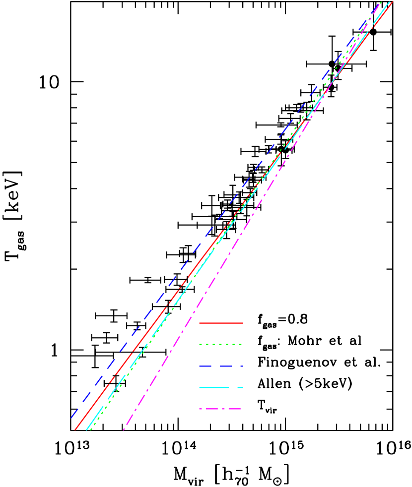
Figure 4: Predicted $M$-$T$ relations compared with observations. Solid and dotted lines indicate the $M$-$T$ relations derived from the observed $L_{\mathrm{X}}$-$T$ relation for $f_{\rm gas}=0.8$ and eq. (18), respectively (corresponding to the crosses in Fig. 3). The observational data points and the fits are taken from Finoguenov et al. (2001; dots with error bars) and Allen et al. (2001; six filled circles with error bars) after correction for the difference of the mass definitions (cf. Appendix A). A simple self-similar model prediction with $T_{\rm gas}=T_{\rm vir}$ is plotted in dot-dashed line for comparison.

Since the $c$-$M_{\rm vir}$ relation has a fairly large intrinsic scatter, we adopt the same value of the power-law index ($-0.13$) as indicated by Bullock et al. (2001), but perform our own fit to their Figure 4 to determine the value of the coefficient $c_{\rm norm}$. In fact, the original coefficient given by Bullock et al. (2001) does not seem to fit their data, and we find $c_{\mathrm{norm}}=8{+2~{}~{}\atop-2.7}$. The quoted errors do not represent the fitting error to the mean relation, but correspond to $\pm 1\;\sigma$ for the intrinsic distribution around the mean relation. The uncertainty with respect to the adopted power-law index ($-0.13$) is effectively included in the above quoted errors for $c_{\rm norm}$. For $\alpha\not=1$, we rescale the amplitude of the concentration parameter according to Keeton & Madau (2001) as $c(M_{\rm vir},z)=(2-\alpha)c_{{B}}(M_{\rm vir},z)$.

The condition that the total mass inside $r_{\rm vir}$ is equal to $M_{\rm vir}$ relates $\delta_{c}$ to $c$ as

$$\delta_{c}(M_{\rm vir})={\Delta_{\rm nl}\over 3}\frac{c^{3}}{m(c)},$$ (5)

where

$$m(x)=\left\{\begin{array}[]{cc}\displaystyle{\ln(1+x)-x/(1+x)}&\alpha=1,\\ \displaystyle 2\left[{\ln(\sqrt{x}+\sqrt{1+x})-\sqrt{\frac{x}{1+x}}}\right]&\alpha=3/2.\end{array}\right.$$ (6)

2.2 Hydrostatic Equilibrium Gas Distribution

We further assume that the intracluster gas is isothermal and in hydrostatic equilibrium, which is a reasonable physical approximation. Under the gravitational potential of the above dark matter halos, the isothermal gas density profiles in hydrostatic equilibrium are computed analytically as (Suto et al., 1998)

$$\rho_{\rm gas}(r)=\rho_{\mathrm{gas},0}\;\exp[-Bf(r/r_{{s}})],$$ (7)

where

$$B=\frac{2c}{m(c)}\frac{T_{\rm vir}}{T_{\rm gas}}$$ (8)

and

$$f(x)=\left\{\begin{array}[]{cc}\displaystyle 1-\frac{1}{x}\ln(1+x)&\alpha=1,\\ \displaystyle 2\sqrt{\frac{1+x}{x}}-\frac{2}{x}\ln(\sqrt{x}+\sqrt{1+x})&\alpha=3/2.\end{array}\right.$$ (9)

In equation (8), $T_{\rm vir}$ is the virial temperature, which we define as

$$k_{\mathrm{B}}T_{\rm vir}=\frac{1}{2}\mu m_{{p}}\frac{GM_{\rm vir}}{r_{\rm vir}}\propto M_{\rm vir}^{2/3},$$ (10)

where $k_{\mathrm{B}}$ is the Boltzmann constant, $G$ is the gravitational constant, and $\mu m_{{p}}$ is the mean molecular weight. We adopt $\mu=0.6$ assuming that the gas is almost fully ionized with the mass fractions of helium $Y=0.24$ and metals $Z=0.3\;Z_{\odot}$ ($Z_{\odot}=0.02$). On the other hand, the gas temperature $T_{\rm gas}$ is determined from the $M$-$T$ relation, as described in detail in §2.3. The central gas density $\rho_{\rm gas,0}$ is computed so that

$$\int_{0}^{r_{\rm vir}}\rho_{\rm gas}(r)4\pi r^{2}dr=f_{\rm gas}M_{\rm vir}\left(\frac{\Omega_{B}}{\Omega_{0}}\right),$$ (11)

where $f_{\rm gas}$ is the hot gas fraction of baryon mass in the cluster described in §2.4. The X-ray luminosity of clusters is computed as

$$L_{\mathrm{X}}=4\pi\int^{r_{\rm vir}}_{0}\Lambda(T_{\rm gas},Z)\left[\frac{\rho_{\rm gas}(r)}{\mu m_{{p}}}\right]^{2}r^{2}dr.$$ (12)

In practice, we adopt the bolometric cooling function of Sutherland & Dopita (1993) for $\Lambda(T_{\rm gas},Z)$.

2.3 Mass-Temperature Relation

As emphasized in the above, we are mainly interested in the $M$-$T$ relation of clusters. Most of previous theoretical studies adopted the self-similar relation for the $M$-$T$ relation: $T_{\rm gas}=T_{\rm vir}\propto M_{\rm vir}^{2/3}$. Recent observations, however, indicate a departure from this relation. Finoguenov et al. (2001), for instance, obtained

$$T_{\rm ew}=(2.63\pm 0.07)\;\mathrm{keV}\left(\frac{M_{500}}{10^{14}\;h_{70}^{-1}\;M_{\odot}}\right)^{0.54\pm 0.02},$$ (13)

where $M_{\Delta_{c}}$ is the total mass enclosed within the radius $r_{\Delta_{c}}$ at which the mean interior density is $\Delta_{c}$ times the critical density of the universe, and $T_{\mathrm{ew}}$ is the emission-weighted temperature. Finoguenov et al. (2001) estimated $M_{500}$ from the observed X-ray luminosity density profile assuming that the gas is in hydrostatic equilibrium. Similarly Allen et al. (2001) found

$$T_{\mathrm{2500}}=(3.38\pm 0.42)\;\mathrm{keV}\left(\frac{M_{2500}}{10^{14}\;h_{70}^{-1}\;M_{\odot}}\right)^{0.65\pm 0.09},$$ (14)

where $T_{2500}$ is the gas-mass–weighted temperature within $r_{2500}$ (see also Ettori, De Grandi, & Molendi, 2002).

In order to generalize the various choices in the $M$-$T$ relation, we adopt the parameterization

$$T_{\rm gas}(M_{\rm vir})=T_{\mathrm{gas,0}}\left(\frac{M_{\rm vir}}{10^{14}\;h_{70}^{-1}\;M_{\odot}}\right)^{p_{\mathit{MT}}}.$$ (15)

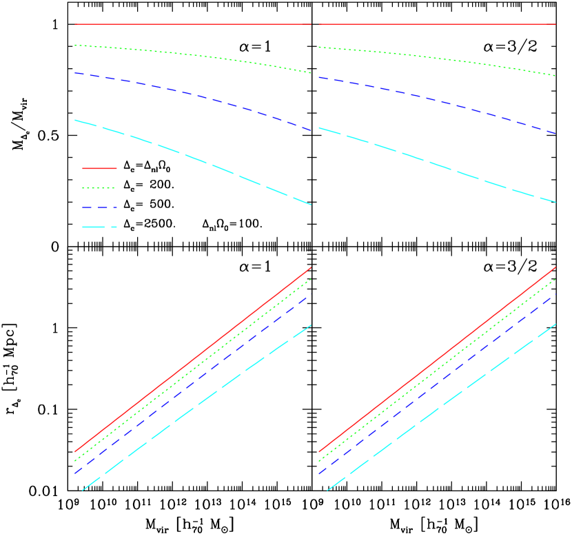
Figure 9: Ratio, $M_{\Delta_{c}}/M_{\rm vir}$ (upper panels) and radius, $r_{\Delta_{c}}$ (lower panels), for a given overdensity $\Delta_{c}$ as a function of $M_{\rm vir}$, $\alpha=1$ (left) and $\alpha=3/2$ (right). Solid, dotted, short-dashed, and long-dashed lines correspond to the overdensities $\Delta_{c}=\Omega_{0}\,\Delta_{\rm nl}$, 200, 500, and 2500, respectively. The standard critical overdensity predicted in the nonlinear spherical collapse model $\Omega_{0}\,\Delta_{\rm nl}$ is $\sim 100$ in our fiducial values of the cosmological parameters with $\Omega_{0}=0.3$ and $\lambda_{0}=0.7$.

For reference, the self-similar model $T_{\rm gas}=T_{\rm vir}$ with equation (10) corresponds to $(T_{\mathrm{gas,0}},p_{\mathit{MT}})=(1.1~{}{\rm keV},\frac{2}{3})$. Since $M_{500}$ and $M_{2500}$ quoted in equations (13) and (14) are different from $M_{\rm vir}$, we translate them to $M_{\rm vir}$, properly taking into account the dark matter density profiles as described in Appendix A (the relations between $M_{\Delta_{c}}$ and $M_{\rm vir}$ for several different values for the overdensity $\Delta_{c}$ are plotted in Fig. 9 below). In doing so, we also convert the cluster data at the individual redshifts into those at $z=0$, taking into account the difference of the Hubble parameter at $z$ and $H_{0}$ for our assumed cosmology ($\Omega_{0}=0.3$, $\lambda_{0}=0.7$, and $h_{70}=1.0$). Then we find that the observed samples are well fitted to the relations

$$T_{\rm gas}=\left\{\begin{array}[]{cc}\displaystyle(1.92\pm 0.06)\;\mathrm{keV}\left(\frac{M_{\rm vir}}{10^{14}\;h_{70}^{-1}\;M_{\odot}}\right)^{0.54\pm 0.02}&\alpha=1,\\ \displaystyle(1.88\pm 0.06)\;\mathrm{keV}\left(\frac{M_{\rm vir}}{10^{14}\;h_{70}^{-1}\;M_{\odot}}\right)^{0.54\pm 0.02}&\alpha=3/2,\\ \end{array}\right.$$ (16)

for Finoguenov et al. (2001), and

$$T_{\rm gas}=\left\{\begin{array}[]{cc}\displaystyle(1.53\pm 0.56)\;\mathrm{keV}\left(\frac{M_{\rm vir}}{10^{14}\;h_{70}^{-1}\;M_{\odot}}\right)^{0.57\pm 0.12}&\alpha=1,\\ \displaystyle(1.45\pm 0.54)\;\mathrm{keV}\left(\frac{M_{\rm vir}}{10^{14}\;h_{70}^{-1}\;M_{\odot}}\right)^{0.59\pm 0.12}&\alpha=3/2,\\ \end{array}\right.$$ (17)

for Allen et al. (2001).

2.4 Hot Gas Mass Fraction

Hot gas fraction $f_{\rm gas}$ also plays a central role in predicting the X-ray luminosity of clusters. In many theoretical analyses, it is often assumed that $f_{\rm gas}$ is independent of the mass of the hosting halos just for simplicity. Of course, this is not a good approximation because the gas in less massive systems is expected to have cooled more efficiently at high redshifts on average, and thus $f_{\rm gas}$ should be a monotonically increasing function of the halo mass. This qualitative feature is supported by both observations and hydrodynamical simulations. Mohr, Mathiesen, & Evrard (1999), for instance, measured the gas mass fraction within $r_{500}$ as a function of gas temperature in the range $3\;\mathrm{keV}\lesssim T_{\rm gas}\lesssim 10\;\mathrm{keV}$. Extrapolating their result to lower temperatures, and assuming for simplicity that the gas mass fraction at the virial radius is equal to that at $r_{500}$, we obtain

$$f_{\rm gas}=\mathrm{min}\left[0.92h_{\rm 70}^{-3/2}\left(\frac{T_{\rm gas}}{6\;\mathrm{keV}}\right)^{0.34},\ 1\right].$$ (18)

This is our fiducial model for the hot gas fraction in the present analysis, and for comparison, we also consider a simple model $f_{\rm gas}=0.8$, in which the gas mass fraction is independent of halo mass and gas temperature.

Strictly speaking, we have to convert the value of the gas fraction of Mohr et al. (1999) defined at $r_{500}$ to that at the virial radius. In practice, however, the observational error of the value is significantly larger than the difference of the conversion, and thus we assume here that $f_{\rm gas}(r_{500})=f_{\rm gas}(r_{\rm vir})$. We put an additional condition that the hot gas to baryon fraction in clusters inside their virial radius does not exceed the cosmological baryon fraction for our assumed cosmological parameters ($\Omega_{0}=0.3$ and $\Omega_{B}=0.04\;h_{70}^{-2}$). In fact, the observed gas to dark matter fraction has a large scatter (see Fig. 14 of Mohr et al. 1999) and is consistent with the upper bound that we set here. Actually, if we adopt the observational $M$-$T$ relation of Finoguenov et al. (2001), we can constrain the gas mass fraction so as to reproduce the observed $L_{\mathrm{X}}$-$T$ relation and XTF. As shown in Appendix B, the resulting constraint is fairly consistent with equation (18).

3 Mass-temperature relation

3.1 Constraints from the Luminosity-Temperature Relation

As mentioned above, the simple self-similar model prediction $L_{\mathrm{X}}\propto T^{2}$ is too shallow to be consistent with the observation ($L_{\mathrm{X}}\propto T^{3}$). This means that heating/cooling processes in addition to the shock heating are important in the thermal evolution of intracluster gas. Apart from the physical mechanism of the additional thermal processes, there are three possibilities that might modify the mass dependence of X-ray luminosity (see eq. [12]) and steepen the resulting $L_{\mathrm{X}}$-$T$ relation. First, the gas density profile may be significantly flatter for less massive systems. Second, the mass dependence of the hot gas mass fraction is strong as $f_{\rm gas}\propto M_{\rm vir}^{1/3}$. Finally, the mass-temperature relation is $T_{\rm gas}\propto M_{\rm vir}^{2/5}$. In practice, a realistic model should be a combination of those three effects to some extent. The gas density profile can be specified completely from the hydrostatic equilibrium assumption. As for the hot gas mass fraction, we adopt the observed relation as well as the simple constant fraction. Then the model described in the previous section enables one to compute the X-ray luminosity of a given halo, and to examine whether the observed $L_{\mathrm{X}}$-$T$ relation can be reproduced from observed $M$-$T$ relation and the gas mass fraction.

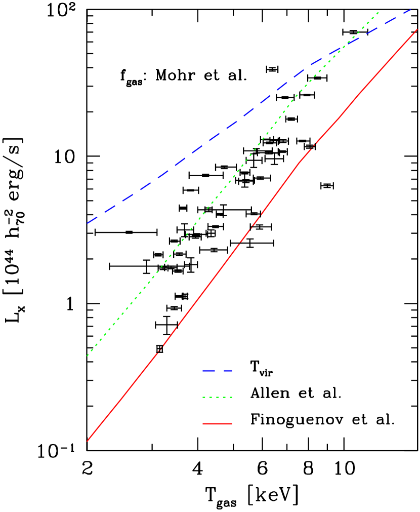
Figure 1: X-ray $L_{\mathrm{X}}$-$T$ relations derived from the observed $M$-$T$ relations (solid line, eq. [16]; dotted line, eq. [17]) assuming the observed gas mass fraction (eq. [18]). A simple self-similar model prediction with $T_{\rm gas}=T_{\rm vir}$ is plotted by the dashed line for comparison. The data with error bars indicate 52 X-ray clusters with temperature higher than 2.5 keV from the sample of Ikebe et al. (2002).

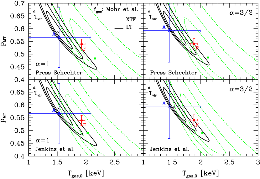
Figure 8: Joint constraints on the parameterized $M$-$T$ relation from the binned $L_{\mathrm{X}}$-$T$ data (solid curves; Fig. 3) and from the XTF (dotted curves; Fig. 5). Upper and lower panels adopt the mass functions of Press & Schechter (1974) and Jenkins et al. (2001), respectively, $\alpha=1$ (Left) and $\alpha=3/2$ (Right). Symbols are as in Figs. 3 and 5.

Before doing so, let us first look at the $L_{\mathrm{X}}$-$T$ relation predicted from the observed $M$-$T$ relations (eqs. [16] and [17]) and gas mass fraction (eq. [18]) combined with the isothermal gas density profile (eq. [7]). Figure 1 compares those predictions against 52 X-ray clusters with temperature higher than 2.5 keV from the sample of Ikebe et al. (2002) (excluding the two clusters with no reliable estimates for their temperatures). For comparison, we also plot the result for the self-similar model (eq. [10]). Incidentally, we performed all the analysis below both for $\alpha=1$ and $3/2$, but their difference turns out to be very small. Thus, we show the results for $\alpha=1$ except for the combined contour plot (see Fig. 8 below).

This clearly illustrates that the predicted $L_{\mathrm{X}}$-$T$ relation is very sensitive to the assumed $M$-$T$ relation; as is well known, the simple self-similar model (Fig. 1, dashed line) is inconsistent with the observations by a wide margin. If the halo density profile is well described by equation (1) with $1\leq\alpha\leq 3/2$, the $M$-$T$ relation of Allen et al. (2001; Fig. 1, dotted line) is in good agreement and that of Finoguenov et al. (2001; solid line) leads to an acceptable result. This conclusion in turn indicates that the $L_{\mathrm{X}}$-$T$ relation provides a good diagnosis of the underlying $M$-$T$ relation, which is as yet poorly determined observationally.

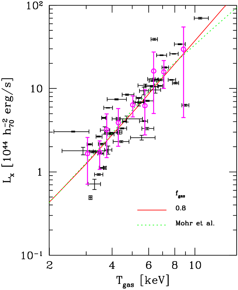
Figure 2: Best-fit $L_{\mathrm{X}}$-$T$ relations from the parameterized $M$-$T$ relations (crosses in Fig. 3). The nine open circles with error bars indicate the binned data described in the text. Solid and dotted lines correspond to the cases assuming the gas mass fraction of $f_{\rm gas}=0.8$ and of equation (18), respectively.

Therefore, we next attempt to find the range of parameters ($p_{\mathit{MT}}$ and $T_{\rm gas,0}$ in eq. [15]) which reproduces the observed $L_{\mathrm{X}}$-$T$ relation. As is clear from Figure 1, the observed data have intrinsic dispersions. Thus, we first divide the cluster sample in nine temperature bins so that each bin contains five or six clusters. Then we compute the mean temperature, and the mean luminosity and the standard deviation of clusters in each bin. The results are plotted by open circles with error bars for the luminosity in Figure 2. Then we perform a $\chi^{2}$ fit to the binned data.

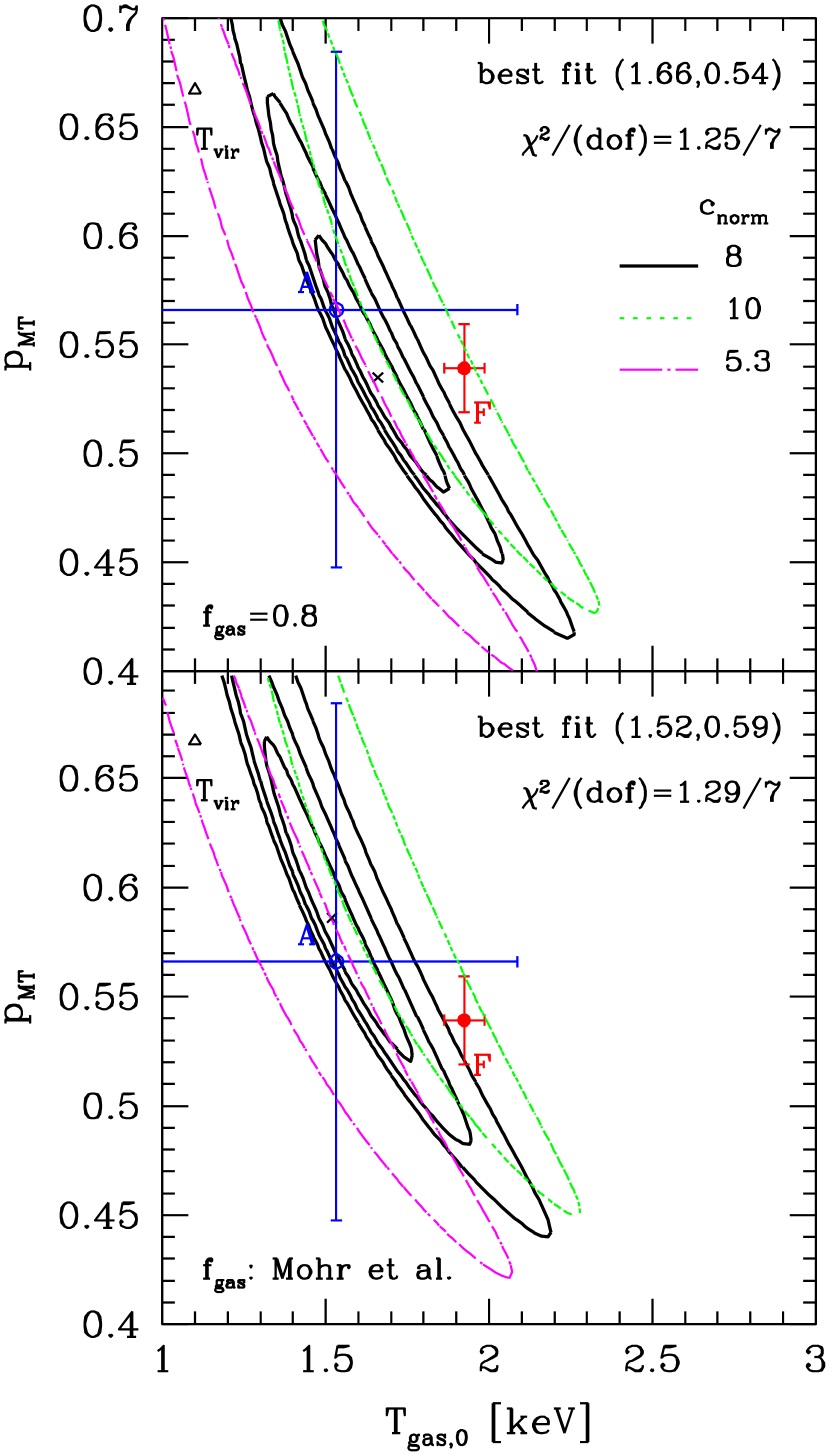
Figure 3: Constraints on the parameterized $M$-$T$ relation of clusters from the $\chi^{2}$ fit to the binned $L_{\mathrm{X}}$-$T$ data. Upper and lower panels adopt the gas mass fraction of $f_{\rm gas}=0.8$ and of eq. (18), respectively. The three contour curves represent the $1\;\sigma$(68.4%), $2\;\sigma$(95.6%), and $3\;\sigma$(99.7%) confidence levels for $c_{\mathrm{norm}}=8$. Crosses show the positions of the best-fit values indicated in each panel. For comparison, also plotted are the self-similar model prediction (open triangles), and observational estimates by Allen et al. (2001; open circles) and Finoguenov et al. (2001; filled circles). Dotted and dot-dashed contours indicate the results of $3\;\sigma$(99.7%) confidence levels for $c_{\mathrm{norm}}=10$ and 5.3, corresponding to $\pm 1\;\sigma$ deviation from the average.

The result is plotted as confidence contours on the $T_{\rm gas,0}$-$p_{\mathit{MT}}$ plane in Figure 3. We estimate the relative confidence levels with respect to the best-fit values assuming that

$$\Delta\chi^{2}\equiv\chi^{2}(T_{\rm gas,0},p_{\mathit{MT}})-\chi^{2}(T_{\rm gas,0,min},p_{\mathit{MT,}{\rm min}})$$ (19)

follows the $\chi^{2}$ distribution of the 2 degrees of freedom (e.g., Press et al., 1992, chap. 15), where $T_{\rm gas,0,min}$ and $p_{\mathit{MT,}{\rm min}}$ are the best-fit parameters that minimize the value of $\chi^{2}$. Upper and lower panels correspond to the gas mass fraction of $f_{\rm gas}=0.8$ and of equation (18) from Mohr et al. (1999). The three contour curves represent the 1, 2, and 3$\;\sigma$ confidence levels derived from the value of $\Delta\chi^{2}$. Crosses show the positions of the best-fit values indicated in each panel. For comparison, we plot the self-similar model prediction, and observational estimates by Allen et al. (2001) and Finoguenov et al. (2001) as open triangles, open circles, and filled circles, respectively. Figure 3 rephrases the visual impression from Figure 1 in a more quantitative way; the $M$-$T$ relation of Allen et al. (2001) is inside the 1$\;\sigma$ contour and that of Finoguenov et al. (2001) is located just outside the 3$\;\sigma$ confidence level, and marginally consistent within the large error-bars. While the concentration parameter of dark matter halos has a fairly broad distribution corresponding to $c_{\mathrm{norm}}=8{+2~{}~{}\atop-2.7}$ in equation (4), it does not lead to any significant difference (compare dotted and dot-dashed lines with solid lines in Fig. 3). Thus, we fix the proportional constant of the concentration parameter $c_{\mathrm{norm}}=8$ in what follows.

The resulting $L_{\mathrm{X}}$-$T$ and $M$-$T$ relations for the best-fit parameters are plotted in Figures 2 and 4. While our best-fit models actually reproduce the observed $L_{\mathrm{X}}$-$T$ relation (the best-fit value of $\chi^{2}$ per degree of freedom is shown in each panel of Fig. 3), they also seem to be in reasonable agreement with the observed $M$-$T$ relation.

3.2 Constraints from X-ray Temperature Function

One can also infer the empirical shape of the $M$-$T$ relation from the requirement that it reproduces the observed XTF of clusters. Comparing with that from the $L_{\mathrm{X}}$-$T$ relation, this methodology provides a fairly (even if not entirely) independent constraint on the $M$-$T$ relation, mainly in two important aspects: (1) the model dependence on the density profile enters only through the flux limit, $S_{\rm lim}$, of the observed sample, and (2) the prediction, on the other hand, is sensitive to the adopted mass function of dark matter halos, and therefore to the value of $\sigma_{8}$ in particular (remember that we fix the other cosmological parameters in the present analysis).

For this purpose, we again use the 54 X-ray clusters with temperature higher than 2.5 keV from the sample of Ikebe et al. (2002). The corresponding flux limit is $S_{\rm lim}=2\times 10^{-11}$ erg s^-1 cm^-2 in the (0.1–2.4) keV band, and the total sky coverage is $8.14$ sr. For definiteness, we adopt the gas mass fraction given by equation (18). As for the halo mass function, we adopt both an analytic model by Press & Schechter (1974) and a fitting model to the numerical simulations by Jenkins et al. (2001),

$$\frac{dn}{d\ln M_{{\mathrm{vir}}}} = \frac{\bar{\rho}}{M_{\mathrm{vir}}}f(\sigma)\frac{d\ln\sigma^{-1}}{d\ln M_{\mathrm{vir}}},$$ (20)

$$f(\sigma) = 0.315\exp\left(-\left|\ln\sigma^{-1}+0.61\right|^{3.8}\right).$$ (21)

We define the rms variance of linear density field $\sigma$ as

$$\sigma^{2}(M)=4\pi\int P(k)\frac{3}{(kR)^{3}}[\sin(kR)-kR\cos(kR)]k^{2}dk,$$ (22)

where $R=(3M/4\pi\bar{\rho})^{1/3}$ and $P(k)$ is the linear power spectrum. We perform the $\chi^{2}$ fit to the data with respect to the three free parameters: $p_{\mathit{MT}}$ and $T_{\rm gas,0}$ in equation (15), and $\sigma_{8}$.

In order to avoid uncertainties in constructing the conventional XTF data (e.g., the definition of $V_{\rm max}$ as discussed by Ikebe et al. 2002), we directly use the number count of clusters with the flux limit $S_{\rm lim}$ per unit solid angle of the sky, appropriated binned according to their temperatures. In practice, we divide both the data and our predictions into five temperature bins (2.5–3.6, 3.6–5.0, 5.0–6.4, 6.4–8.0, and $>$8.0 keV), so that the errors do not correlate with one another, and perform the $\chi^{2}$ fit. We assign the Poisson error to the number count in each bin.

The result is plotted as confidence contours on the $T_{\rm gas,0}$-$p_{\mathit{MT}}$ plane in Figure 5. Again we estimate the relative confidence levels with respect to the best-fit values assuming that

$$\Delta\chi^{2}\equiv\chi^{2}(T_{\rm gas,0},p_{\mathit{MT}},\sigma_{\mathrm{8,local}\ \mathrm{min}})-\chi^{2}(T_{\rm gas,0,min},p_{\mathit{MT,}\mathrm{min}},\sigma_{\rm 8,min})$$ (23)

follows the $\chi^{2}$ distribution of the 2 degrees of freedom, where $T_{\rm gas,0,min}$, $p_{\mathit{MT,}\mathrm{min}}$ and $\sigma_{\rm 8,min}$ are the best-fit parameters that minimize the value of $\chi^{2}$, and $\sigma_{\mathrm{8,local}\ \mathrm{min}}$ is the value of $\sigma_{8}$ minimizing the $\chi^{2}$ with given $T_{\rm gas,0}$, and $p_{\mathit{MT}}$. Upper and lower panels of Figure 5 correspond to the mass functions of Press & Schechter (1974) and Jenkins et al. (2001), respectively. The three solid contour curves represent the 1, 2, and 3$\;\sigma$ confidence levels derived from the $\chi^{2}$ fit, with the filled squares indicating the points of the highest significance. Dotted contours, on the other hand, indicate the best-fit value of $\sigma_{8}$ at the given location on the $T_{\rm gas,0}$-$p_{\mathit{MT}}$ plane. The self-similar model prediction, and observational estimates by Allen et al. (2001) and Finoguenov et al. (2001), are plotted by open triangles, open circles, and filled circles, respectively.

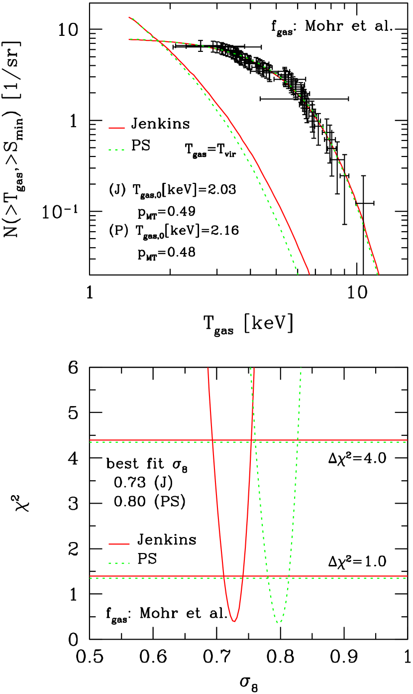
Figure 6: Best-fit XTF (upper panel) from the parameterized $M$-$T$ relation compared to the cluster sample of Ikebe et al. (2002) and the corresponding $\chi^{2}$ as a function of $\sigma_{8}$ (lower panel). Solid and dotted curves adopt the mass functions of Jenkins et al. (2001) and Press & Schechter (1974), respectively. A simple self-similar model prediction with $T_{\rm gas}=T_{\rm vir}$ is also plotted just for illustration.

The upper panel in Figure 6 illustrates that the best-fit model reproduces the observed XTF nicely. Again just for comparison, we plot the self-similar model predictions, which do not fit the observed XTF at all. Moreover, the lower panel indicates that the degree of fit is indeed sensitive to the value of $\sigma_{8}$; the best-fit value is 0.7–0.8.

Although the above conclusion may seem inconsistent with the previous claims (Viana & Liddle 1996; Eke, Cole, & Frenk 1996; Kitayama & Suto 1997) that the self-similar model does fit the observed XTF with $\sigma_{8}=0.9\mbox{--}1.0$, it can be explained by the following reasons. First, the previous XTF data had much larger errors and thus still allowed a wider range of theoretical models. Second, the latest XTF data that we adopted have a systematically smaller amplitude at $T_{\rm gas}>5\;$keV than the previous ones (see Fig. 6 of Ikebe et al., 2002). Third, the adopted $L_{\mathrm{X}}$-$T$ relation is different; our current self-similar model corresponds to $L_{\mathrm{X}}\propto T_{\rm gas}^{2}$, while the previous analyses used (sometimes implicitly) $L_{\mathrm{X}}\propto T_{\rm gas}^{3}$ to construct the “observed” XTF data via the conventional $V_{\rm max}$ method (e.g., Eke et al., 1996). Finally, the recent mass function of Jenkins et al. (2001) predicts more massive halos than that of Press & Schechter (1974), which has been widely used in the previous analyses.

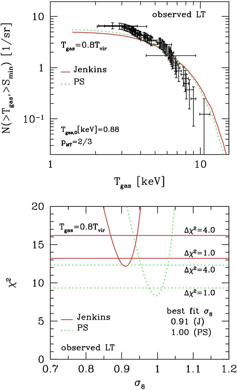
Figure 7: Same as Fig. 6, but for a self-similar model adopting the observed $L_{\mathrm{X}}$-$T$ relation and a slightly smaller proportional factor ($T_{\rm gas}=0.8T_{\rm vir}$).

Figure 7 demonstrates the above features. For a direct comparison with the analyses of Kitayama & Suto (1997), we adopt $T_{\rm gas}=0.8T_{\rm vir}$ and the $L_{\mathrm{X}}$-$T$ relation from equation (3) of Kitayama & Suto (1997), with their fiducial choice for the other parameters. The goodness of the fit turns out to be significantly degraded compared to the previous result, mainly because of the systematically smaller amplitude of the XTF, as well as reduced error bars. Nevertheless, this methodology fully reproduces the best-fit value of $\sigma_{8}=0.9\mbox{--}1.0$, as in the previous one.

In fact, the combination of those effects also explains why the reanalysis of the cluster abundance by Seljak (2002) yielded $\sigma_{8}\sim 0.7$ in the standard $\Lambda$CDM model when adopting the $M$-$T$ relation of Finoguenov et al. (2001). Incidentally, the smaller value of $\sigma_{8}$ seems consistent with the recent joint analysis of cosmic microwave background and large-scale structure (Efstathiou et al., 2002), which suggests $\sigma_{8}=0.6\mbox{--}0.7$.

4 Discussion and conclusions

We have presented the constraints on the (empirically parameterized) mass-temperature relation of galaxy clusters from the two different observational data, the luminosity-temperature relation and the temperature function.

We summarize in Figure 8 our constraints on the $T_{\rm gas,0}$-$p_{\mathit{MT}}$ plane, adopting the observed gas mass fraction (eq. [18]). The fact that the simple self-similar evolution model $T_{\rm gas}\propto M_{\rm vir}^{2/3}$ fails to explain the observed $L_{\mathrm{X}}$-$T$ relation is well known and not at all new. Rather, it should be noted that the mass-temperature relation of galaxy clusters is fairly well constrained by combining the observed $L_{\mathrm{X}}$-$T$ relation and XTF. It is encouraging that $T_{\rm gas}=(1.5\sim 2.0)\;{\rm keV}(M_{\rm vir}/10^{14}\;h_{70}^{-1}\;M_{\odot})^{0.5\sim 0.55}$ barely satisfy the two constraints simultaneously. This conclusion applies for $1\leq\alpha\leq 3/2$ as long as the dark halo density profile is described by equation (1).

In addition, our analysis implies that the amplitude of the mass variance $\sigma_{8}$ in the standard $\Lambda$CDM model should be 0.7–0.8. These values are significantly smaller than the previous estimates (Viana & Liddle, 1996; Eke et al., 1996; Kitayama & Suto, 1997) but in better agreement with more recent results (Seljak, 2002; Efstathiou et al., 2002).

Since our current analysis has adopted a simple parameterized model for the mass-temperature relation, the result should be understood by a physical model of the thermal evolution of the intracluster gas. For instance, our result may be qualitatively explained by a kind of phenomenological heating of $T_{\rm gas}(M_{\rm vir})=T_{\rm vir}(M_{\rm vir})+1\;$keV. We plan to examine the implications for the possible heating sources from the derived mass-temperature relation of galaxy clusters using the Monte-Carlo modeling of merger trees.

Appendix A Mass-radius relation at a given overdensity

In order to determine the mass of a cluster, one has to specify the radius from its center. Observationally, this is often set by the specific fractional overdensity $\Delta_{c}$ with respect to the critical density of the universe, $\rho_{c}$. Thus the resulting mass $M_{\Delta_{c}}$ is written in terms of the corresponding radius $r_{\Delta_{c}}$ as

$$M_{\Delta_{c}}=\frac{4}{3}\pi r_{\Delta_{c}}^{3}\Delta_{c}\rho_{c}.$$ (A1)

Most theoretical studies, on the contrary, usually define the mass of dark matter halo $M_{\rm vir}$ at its virial radius $r_{\rm vir}$, adopting the spherical nonlinear collapse model, i.e., $\Delta_{c}=\Omega_{0}\Delta_{\rm nl}(\Omega_{0},\lambda_{0})$ (see Kitayama & Suto 1996 for details).

Once the density profile of dark matter halos is specified, $M_{\Delta_{c}}$ can be easily translated into $M_{\rm vir}$. For the profile that we adopted in this paper (eq. [1]), mass inside a radius $r$ is written as

$$M(r)=4\pi\delta_{c}\bar{\rho}(z)r_{{s}}^{3}m(r/r_{{s}}),$$ (A2)

where $m(x)$ is defined in equation (6). Thus, if $\Delta_{\rm c}$ is given, one can compute $r_{\Delta_{c}}$ and $M_{\Delta_{c}}/M_{\rm vir}$ from the following relation

$$\frac{M_{\Delta_{c}}}{M_{\rm vir}}=\frac{m(r_{\Delta_{c}}/r_{\mathrm{s}})}{m(c)}=\frac{r_{\Delta_{c}}^{3}}{r_{\rm vir}^{3}}\frac{\Delta_{c}}{\Delta_{\mathrm{nl}}}\frac{\rho_{c}}{\bar{\rho}}.$$ (A3)

Figure 9 plots $M_{\Delta_{c}}/M_{\rm vir}$ (upper panels) and $r_{\Delta_{c}}$ (lower panels) for several choices of $\Delta_{c}$.

Appendix B Hot gas mass fraction

The strategy that we have adopted in the present paper is to determine the permitted parameter region of the $M$-$T$ relation of clusters from the $L_{\mathrm{X}}$-$T$ relation and XTF, assuming a specific model for the hot gas mass fraction $f_{\rm gas}(M_{\rm vir})$ inspired by the observation. In principle, however, we may repeat the similar procedure and derive the constraints on $f_{\rm gas}(M_{\rm vir})$, assuming the observed $M$-$T$ relation instead. Since the observational uncertainty for the hot gas mass fraction (eq. [18]) that we adopted is fairly large, this approach is useful in understanding the dependence of our conclusion on the model for the gas mass fraction.

For this purpose, we also parameterize the gas mass fraction by a single power law,

$$f_{\rm gas}(T_{\rm gas})=f_{\mathrm{gas},0}\left(\frac{T_{\rm gas}}{1\;\mathrm{keV}}\right)^{p_{\scriptscriptstyle\rm gas}},$$ (B1)

and perform the $\chi^{2}$ fit to the $L_{\mathrm{X}}$-$T$ relation varying the two free parameters, $f_{\mathrm{gas},0}$ and $p_{\rm gas}$. We repeat the similar fitting XTF with $f_{\mathrm{gas},0}$, $p_{\rm gas}$ and $\sigma_{8}$.

The result is plotted in Figure 10, where we use the observed $M$-$T$ relation of Finoguenov et al. (2001). Solid contour curves represent the 1, 2, and 3$\;\sigma$ confidence levels derived from the $\chi^{2}$ fit to the $L_{\mathrm{X}}$-$T$ relation, while dotted curves show the 1, 2, and 3$\;\sigma$ confidence levels from the XTF. Clearly, both constraints again are simultaneously satisfied for $f_{\rm gas}=(0.5\pm 0.1)(T_{\rm gas}/1\;{\rm keV})^{0.4\pm 0.15}$, and in fact agree with the observed gas mass fraction of Mohr et al. (1999). We also plot the condition that $f_{\rm gas}(10\;{\rm keV})=1$ by a dashed line, so that the hot gas fraction does not exceed the cosmological average of the baryon fraction (assuming that $\Omega_{B}=0.04\;h_{70}^{-1}$ and $\Omega_{0}=0.3$). If this condition should be satisfied, the acceptable parameter range almost exactly corresponds to the observed gas mass fraction of Mohr et al. (1999).

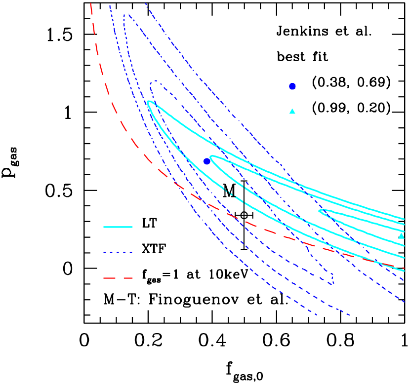
Figure 10: Joint constraints on the parameterized hot gas mass fraction relation from the observed $L_{\mathrm{X}}$-$T$ relation (solid curves) and from the XTF (dotted curves). The fit to the observational data by Mohr et al. (1999) is indicated as an open circle with error bars. Dashed lines indicate the condition that $f_{\rm gas}(10\;{\rm keV})=1$.

References

- Allen et al. (2001) Allen, S. W., Schmidt, R. W., & Fabian, A. C. 2001, MNRAS, 328, L37
- Arnaud & Evrard (1999) Arnaud, M., & Evrard, E. 1999, MNRAS, 305, 631
- Bullock et al. (2001) Bullock, J. S., Kolatt, T. S., Sigad, Y., Somerville, R. S., Kravtsov, A. V., Klypin, A. A., Primack, J. R., & Dekel, A. 2001, MNRAS, 321, 559
- David et al. (1993) David, L. P., Slyz, A., Jones, C., Forman, W., Vrtilek, S. D., & Arnaud, K. A. 1993, ApJ, 412, 479
- Efstathiou et al. (2002) Efstathiou, G. et al. 2002, MNRAS, 330, L29
- Eke et al. (1996) Eke, V. R., Cole, S., & Frenk, C. S. 1996, MNRAS, 282, 263
- Ettori et al. (2002) Ettori, S., De Grandi, S., & Molendi, S. 2002, A&A, 391, 841
- Evrard & Henry (1991) Evrard, A. E., & Henry, J. P. 1991, ApJ, 383, 95
- Finoguenov et al. (2001) Finoguenov, A., Reiprich, T. H., & Böhringer, H. 2001, A&A, 368, 749
- Fukushige & Makino (2001) Fukushige, T., & Makino, J. 2001, ApJ, 557, 533
- Ikebe et al. (2002) Ikebe, Y., Reiprich, T. H., Böhringer, H., Tanaka, Y., & Kitayama, T. 2002, A&A, 383, 773
- Jenkins et al. (2001) Jenkins, A. Frenk, C. S., White, S. D. M., Colberg, J. M., Cole, S., Evrard, A. E., Couchman, H. M. P., & Yoshida, N. 2001, MNRAS, 321, 372
- Jing & Suto (2000) Jing, Y. P., & Suto, Y. 2000, ApJ, 529, 69
- Kaiser (1986) Kaiser, N. 1986, MNRAS, 222, 323
- Kaiser (1991) Kaiser, N. 1991, ApJ, 383, 104
- Keeton & Madau (2001) Keeton, C. R., & Madau, P. 2001, ApJ, 549, L25
- Kitayama & Suto (1996) Kitayama, T., & Suto, Y. 1996, ApJ, 469, 480
- Kitayama & Suto (1997) Kitayama, T., & Suto, Y. 1997, ApJ, 490, 557
- Markevitch (1998) Markevitch, M. 1998, ApJ, 504, 27
- Makino et al. (1998) Makino, N., Sasaki, S., & Suto, Y. 1998, ApJ, 497, 555
- Mohr et al. (1999) Mohr, J. J., Mathiesen, B., & Evrard, A. E. 1999, ApJ, 517, 627
- Moore et al. (1998) Moore, B., Governato, F., Quinn, T., Stadel, J., & Lake, G. 1998, ApJ, 499, 5
- Navarro et al. (1996) Navarro, J. F., Frenk, C. S., & White, S. D. M. 1996, ApJ, 462, 563
- Press & Schechter (1974) Press, W. H., & Schechter, P. 1974, ApJ, 187, 425
- Press et al. (1992) Press, W. H., Teukolsky, S. A., Vetterling, W. T., & Flannery, B. P. 1992, Numerical Recipes in Fortran, 2nd edition (Cambridge University Press: London)
- Seljak (2002) Seljak, U. 2002, MNRAS, 337, 769
- Sutherland & Dopita (1993) Sutherland, R. S., & Dopita, M. A. 1993, ApJS, 88, 253
- Suto et al. (1998) Suto, Y., Sasaki, S., & Makino, N. 1998, ApJ, 509, 544
- Viana & Liddle (1996) Viana, P. T. P., & Liddle, A. R. 1996, MNRAS, 281, 323