Observational constraints on the curvaton model of inflation

Abstract

Simple curvaton models can generate a mixture of of correlated primordial adiabatic and isocurvature perturbations. The baryon and cold dark matter isocurvature modes differ only by an observationally null mode in which the two perturbations almost exactly compensate, and therefore have proportional effects at linear order. We discuss the CMB anisotropy in general mixed models, and give a simple approximate analytic result for the large scale CMB anisotropy. Working numerically we use the latest WMAP observations and a variety of other data to constrain the curvaton model. We find that models with an isocurvature contribution are not favored relative to simple purely adiabatic models. However a significant primordial totally correlated baryon isocurvature perturbation is not ruled out. Certain classes of curvaton model are thereby ruled out, other classes predict enough non-Gaussianity to be detectable by the Planck satellite. In the appendices we review the relevant equations in the covariant formulation and give series solutions for the radiation dominated era.

I Introduction

Recent detailed measurements of the acoustic peaks in CMB anisotropy power spectrum by the WMAP satellite G. Hinshaw et al. (2003); H. V. Peiris et al. (2003) are consistent with the standard model of a predominantly adiabatic, approximately scale invariant primordial power spectrum in a spatially flat Universe. Frequently it is assumed the initial power spectrum is entirely adiabatic, though there is still no compelling justification for this assumption. Although adiabatic perturbations are predicted from single field models of inflation Liddle and Lyth (2000), if one allows the possibility of multiple fields in the early Universe then there is also the possibility of isocurvature perturbations (also known as entropy perturbations) Kofman and Linde (1987); Polarski and Starobinsky (1994); Garcia-Bellido and Wands (1996); Linde and Mukhanov (1997); Sasaki and Tanaka (1998); Langlois (1999); Gordon et al. (2001); Hwang and Noh (2000); Starobinsky et al. (2001); Bartolo et al. (2001); Groot Nibbelink and van Tent (2002); Wands et al. (2002); Tsujikawa et al. (2002). In particular, the recently proposed curvaton model uses a second scalar field (the ‘curvaton’) to form the perturbations Mollerach (1990); Lyth and Wands (2002); Lyth et al. (2003); Moroi and Takahashi (2001, 2002); Moroi and Murayama (2003). The motivation for this is it makes it easier for otherwise satisfactory particle physics models of inflation to produce the correct primordial spectrum of perturbations Dimopoulos and Lyth (2002). Various candidates for the curvaton have been proposed Postma (2003); Enqvist et al. (2003); Bastero-Gil et al. (2002); Dimopoulos et al. (2003a, b). A curvaton mechanism has also been considered in the pre big bang scenario Copeland et al. (1997); Lidsey et al. (2000); Enqvist and Sloth (2002); Sloth (2003); Bozza et al. (2002) where it can be used to produce an almost scale invariant spectrum.

The curvaton scenario also has the feature of being able to generate isocurvature perturbations of a similar magnitude to the adiabatic perturbation without fine tuning, and therefore is open to observational test.

Early studies of non-adiabatic perturbations, either considered purely isocurvature cold dark matter perturbations Efstathiou and Bond (1986) or mixtures of adiabatic and uncorrelated cold dark matter isocurvature perturbations R. Stompor et al. (1996); Pierpaoli et al. (1999); Kawasaki and Takahashi (2001); Enqvist et al. (2000). However, as first realized by Langlois Langlois (1999), the adiabatic and isocurvature components can be correlated and this correlation may have interesting observational consequences Langlois and Riazuelo (2000). In Ref. Bucher et al. (2001a) they identified four regular isocurvature modes, which in general can have arbitrary correlations with each other and with the adiabatic mode. Such general models have many degeneracies and are badly constrained by pre-WMAP data Trotta et al. (2001, 2003). Detailed CMB polarization data is expected to help with this Bucher et al. (2001b). In Ref. H. V. Peiris et al. (2003) (following Ref. Amendola et al. (2002) with pre-WMAP data) they considered a CDM isocurvature mode with an arbitrary correlation to an adiabatic mode and found that though not favored by the data, a significant isocurvature contribution was still permitted. Constraints on a specific model that doesn’t produce isocurvature modes were given in Ref. Bartolo and Liddle (2002).

Here we start in Section II by making some general remarks about mixed isocurvature models, and discuss the corresponding CMB power spectra predictions. Then in Section III we discuss current observational constraints on totally correlated (or anti-correlated) adiabatic and isocurvature perturbations, as predicted by the curvaton model. Various scenarios within the curvaton model predict specific ratios of adiabatic and isocurvature perturbations, and can be tested directly. In general we find constraints on when the curvaton decayed.

We use the CMB temperature and temperature-polarization cross-correlation anisotropy power spectra from the WMAP L. Verde et al. (2003); G. Hinshaw et al. (2003); A. Kogut et al. (2003) observations, as well as seven almost independent temperature band powers from ACBAR C.L. Kuo et al. (2002) on smaller scales. In addition we use data from the 2dF galaxy redshift survey W. Percival et al. (2002), HST Key Project W. L. Freedman et al. (2001), and nucleosynthesis Burles et al. (2001) using a slightly modified version of the CosmoMC Markov-Chain Monte Carlo program, as described in Ref. Lewis and Bridle (2002).

For simplicity we assume a flat universe with a cosmological constant, uninteracting cold dark matter, and massless neutrinos evolving according to general relativity.

II Primordial perturbations and the CMB anisotropy

It is well known that the curvature perturbation, in the constant density or comoving frame (gauge) is conserved on super-Hubble scales for adiabatic perturbations Bardeen (1980); Bardeen et al. (1983); Lyth (1985); Kodama and Sasaki (1984); Mukhanov et al. (1992). This is not the case in the presence of isocurvature modes since these source changes to the curvature perturbation. However, as shown in Ref. Wands et al. (2000) (and reviewed in Appendix A), in the presence of isocurvature modes the large scale evolution can still be analysed easily using the curvature perturbation in the frame in which the density is unperturbed, $\zeta$. This can be expressed in terms of the curvature perturbations in the frames in which individual species are unperturbed $\zeta_{i}$ using

$$\zeta=\frac{\sum_{i}\rho_{i}^{\prime}\zeta_{i}}{\sum_{i}\rho_{i}^{\prime}},$$ (1)

where the dash denotes the derivative with respect to conformal time. For non-interacting conserved particle species the individual $\zeta_{i}$ are conserved on large scales if there is a definite equation of state $p_{i}=p_{i}(\rho_{i})$. In this case the evolution of $\zeta$ follows straightforwardly from Eq. (1) depending on the evolution of the background energy densities. An adiabatic perturbation is one in which $\zeta_{i}=\zeta$ for all $i$, in which case $\zeta$ is constant in time on large scales. The isocurvature perturbations are defined as Malik et al. (2003)

$$\mbox{$\cal S$}_{i,j}\equiv 3(\zeta_{i}-\zeta_{j})=-3{\cal H}\left(\frac{{\delta\rho}_{i}}{\rho_{i}^{\prime}}-\frac{{\delta\rho}_{j}}{\rho_{j}^{\prime}}\right)$$ (2)

where ${\delta\rho}_{i}=\rho_{i}\Delta_{i}$ (no sum) is the density perturbation in any frame and ${\cal H}$ is the conformal Hubble rate. We consider a fluid consisting of photons ($\gamma$), massless neutrinos ($\nu$), cold baryons ($b$) and cold dark matter (CDM, $c$), where it is conventional to describe the perturbations with $j=\gamma$, in which case the second index can be omitted so $\mbox{${\cal S}_{b}$}\equiv\mbox{$\cal S$}_{b,\gamma}$, etc. The isocurvature perturbations are conserved on large scales where the photon-baryon coupling is unimportant. The $\zeta_{i}$ are related to the fractional density perturbations in the unperturbed curvature frame by $\hat{\Delta}_{i}=3(1+p_{i}/\rho_{i})\zeta_{i}$, and for matter with constant equation of state $\hat{\Delta}_{i}$ are also conserved on large scales.

In general isocurvature perturbations give rise to perturbations in the density, and the universe is no longer exactly FRW. One exception to this is when the two matter perturbations exactly compensate, so ${\delta\rho}_{c}=-{\delta\rho}_{b}$, in which case the total matter density is unperturbed, and hence the universe evolves as though there were no perturbations. In such a universe the CMB anisotropy would be dominated by tiny small scale linear effects due to non-zero pressure of the baryons or dark mater, and second order effects due to the perturbation in the electron number density associated with the baryons. At linear order ${\delta\rho}_{c}=-{\delta\rho}_{b}$, $\zeta={\delta\rho}_{\gamma}={\delta\rho}_{\nu}=0$ is a time independent solution to the pressureless perturbation equations, and adding this solution to any other solution will make no difference to the linear CMB anisotropy or matter power spectrum. It follows that an initial isocurvature perturbation with $\mbox{${\cal S}_{b}$}=1,\mbox{${\cal S}_{c}$}=0$ is observationally essentially indistinguishable from one with $\mbox{${\cal S}_{b}$}=0,\mbox{${\cal S}_{c}$}=\rho_{b}/\rho_{c}$.

We now derive an approximate analytic form for the large scale CMB temperature anisotropy in the presence of primordial isocurvature and adiabatic perturbations. Neglecting a local monopole and dipole contribution, taking recombination to be instantaneous at at conformal time $\tau_{*}$, and assuming the reionization optical depth is negligible, the monopole and Integrated Sachs Wolfe (ISW) contributions to the temperature anisotropies due to scalar perturbations are given by

$$\frac{\delta T}{T}\approx\left[\frac{1}{4}\hat{\Delta}_{\gamma}+2\phi\right]_{\tau_{*}}+2\int_{\tau_{*}}^{\tau_{0}}\phi^{\prime}\,d\lambda,$$ (3)

where $\phi$ is the Weyl potential (see Appendix A) and $\tau_{0}$ is the conformal time today and the integral is along the comoving photon line of site. Additional terms which arise due to the velocities, quadrupoles and polarization at last scattering are generally sub-dominant on large scales. Since the pressures are assumed to be zero the perturbations are purely adiabatic in the matter era, and hence $\zeta$ is constant on large scales. During matter domination the potential evolves as $\phi=C_{1}+C_{2}/\tau^{5}$, and can be related to $\zeta$ using Eq. (34) when the anisotropic stress is negligible

$$\phi=-\frac{3}{5}\zeta+\frac{C_{2}}{\tau^{5}}.$$ (4)

Since the radiation to matter density ratio only falls off as $\sim 1/\tau^{2}$ when the matter dominates, when the approximation of matter domination is accurate it should also be valid to neglect the decaying mode $\propto 1/\tau^{5}$ and assume $\phi\approx-\frac{3}{5}\zeta$. Using $\hat{\Delta}_{\gamma}=4\zeta_{\gamma}$, and neglecting the ISW contribution Eq. (3) then becomes

$$\frac{\delta T}{T}\approx\zeta_{\gamma}-\frac{6}{5}\zeta$$ (5)

where from Eq. (1) in matter domination

$$\zeta\approx R_{b}\zeta_{b}+R_{c}\zeta_{c}.$$ (6)

Here we define the matter fractions $R_{b}\equiv\rho_{b}/\rho_{m}$, $R_{c}\equiv\rho_{c}/\rho_{m}$, where $\rho_{m}=\rho_{c}+\rho_{b}$.

During early radiation domination $\zeta^{\text{rad}}\approx R_{\gamma}\zeta_{\gamma}+R_{\nu}\zeta_{\nu}$ from Eq. (1), where we define the radiation density fractions $R_{\nu}\equiv\rho_{\nu}/(\rho_{\gamma}+\rho_{\nu}),R_{\gamma}\equiv\rho_{\gamma}/(\rho_{\gamma}+\rho_{\nu})$. Using Eqs. (2) and (5) and the constancy of the large scale $\zeta_{i}$ we can therefore relate the large scale temperature anisotropy to the primordial adiabatic and isocurvature perturbations

$$\frac{\delta T}{T}\approx-\frac{1}{5}\zeta^{\text{rad}}-\frac{2}{5}\left(R_{c}\mbox{${\cal S}_{c}$}+R_{b}\mbox{${\cal S}_{b}$}\right)+\frac{1}{15}R_{\nu}\mbox{$\cal S_{\nu}$}.$$ (7)

We can take $\zeta^{\text{rad}}$ as a measure of the primordial adiabatic perturbation. So this formula shows the effect of a mixture of adiabatic and isocurvature perturbations on the observed large scale CMB temperature anisotropy. This result agrees with that in Langlois and Riazuelo (2000), despite errors in their derivation which arise from an invalid ansatz for the time evolution of the velocities and anisotropic stress (demonstrated by counterexample in Appendix B). However in matter domination the velocities are negligible so the error is harmless, and for the adiabatic and neutrino modes the assumption is correct to the required order during radiation domination. However unfortunately their general result for the evolution of the potential is incorrect and cannot be used to improve on the above much simpler argument.

This analytic argument shows the main qualitative features, though in reality recombination is far from being completely matter dominated, and the ISW and other contributions will not be negligible. It is however straightforward to compute the CMB and matter power spectra numerically Seljak and Zaldarriaga (1996); Lewis et al. (2000) starting from a series solution in the early radiation dominated era (Appendix B).

III Constraining the Curvaton model

The curvaton scenario provides a mechanism for allowing the inflation potential to have more natural properties, at the expense of introducing an additional unidentified scalar field which generates the perturbations. In the curvaton model the inflaton field drives the initial expansion and generates an era of radiation domination after it decays. The expansion rate then slows and the curvaton field can reach the minimum of its potential and start to oscillate. During oscillation the curvaton field acts effectively like a matter component, and its perturbation acts like a matter isocurvature mode. As the radiation redshifts further the equation of state then changes to matter domination as the curvaton density comes to dominate. As the background equation of state changes, a curvature perturbation is generated from the isocurvature mode. The curvaton then decays into (predominantly) radiation well before nucleosynthesis, and we enter the usual primordial radiation dominated epoch.

Primordial correlated isocurvature modes can be generated if the baryons or CDM are generated by, or before, the curvaton decays, as discussed in detail below. If one or both were created before the curvaton decays, the current model assumes that the curvaton had a negligible density when they decayed Lyth et al. (2003). We assume that the curvaton is the only cosmologically relevant scalar field after inflaton decay, and that the perturbations in the inflaton field are negligible. Generically such models predict a very small tensor mode contribution, which we assume can be neglected. We assume there is no lepton number at neutrino decoupling so that there are no neutrino isocurvature modes, though see Lyth et al. (2003) for other possibilities.

As discussed in Section II, the baryon and CDM isocurvature modes predict proportional results, so we can account for ${\cal S}_{c}$ by using just an effective baryon isocurvature perturbation

$$\mbox{$\cal S$}^{\text{eff}}_{{b}}=\mbox{${\cal S}_{b}$}+\frac{R_{c}}{R_{b}}\mbox{${\cal S}_{c}$}.$$ (8)

The baryon and CDM isocurvature perturbations are completely correlated (or anti-correlated) with each other and the adiabatic perturbation, so $\mbox{$\cal S$}^{\text{eff}}_{{b}}=B\zeta^{\text{rad}}$ where $B$ measures the isocurvature mode contribution and is taken to be scale independent. From Eq. (7), the large scale CMB anisotropy variance is then given approximately by

$$\left\langle\frac{\delta T^{2}}{T^{2}}\right\rangle\approx\frac{1}{25}(1+2R_{b}B)^{2}{\cal P}_{\zeta},$$ (9)

where ${\cal P}_{\zeta}={\cal P}_{\zeta}^{\text{rad}}$ is the initial power spectrum. We assume ${\cal P}_{\zeta}$ is well parameterized by ${\cal P}_{\zeta}=A_{s}(k/k_{0})^{n_{s}-1}$ where $A_{s}$ gives the normalization, $n_{s}$ is the scalar spectral index and $k_{0}$ is a choice of normalization point. Note that our number of degrees of freedom is actually less than generic inflation, because although we have introduced $B$ we now no longer have the amplitude and slope of the tensor component to consider. The slope of the isocurvature perturbation is predicted to be the same as the adiabatic perturbation and the tensors are predicted to be negligible in the curvaton scenario Lyth et al. (2003).

The isocurvature modes have little effect on small scales, but as can be seen from Eq. (9) they can either raise or lower the Sachs Wolfe plateau relative to the acoustic peaks depending on the sign of $B$. This is in contrast to tensor perturbations which can only raise the Sachs Wolfe plateau relative to the acoustic peaks.

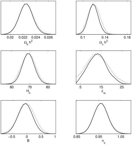
Figure 1: Posterior marginalized probability distributions (solid lines) of the cosmological parameters including correlated matter isocurvature modes, using the data described in the text. $B$ is the ratio of the (effective) baryon isocurvature to adiabatic perturbation amplitude in the primordial era, $\mbox{$\Omega_{b}$}h^{2}$ and $\mbox{$\Omega_{c}$}h^{2}$ are the physical matter densities in baryons and CDM, $H_{0}~{}\text{km}~{}\text{s}^{-1}\text{Mpc}^{-1}$ is the Hubble parameter today, $z_{\text{re}}$ is the effective reionization redshift, and $n_{s}$ is the spectral index. We assume a flat universe with cosmological constant. Dotted lines show the mean likelihoods of the samples, and agree well with the marginalized curves, indicating the full distribution is fairly Gaussian and unskewed Lewis and Challinor (2002).

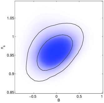
Figure 2: Posterior distribution of $B=\mbox{$\cal S$}^{\text{eff}}_{{b}}/\zeta$ in the primordial era, and the spectral index $n_{s}$. The plot is generated from a smoothed number density of Monte Carlo samples generated using the data described in the text. The contours enclose $68\%$ and $95\%$ of the probability, and the shading is by the mean likelihood of the samples.

Computing the full predictions numerically and assuming a flat prior on $B$, Fig. 1 shows the posterior distribution for the various cosmological parameters when the possibility of a totally correlated mixture of matter isocurvature and adiabatic perturbations is allowed. The posterior distribution of $B$ and $n_{s}$ is shown in Fig. 2, marginalized over the other parameters. On small scales the isocurvature modes have only a small effect, so the main observational constraint comes from the relative amplitudes of the large and small scale power. This is partially degenerate with the spectral index as clearly demonstrated in the figure. The relative large scale amplitude is also affected by the reionization optical depth, and although this is constrained by WMAP’s polarization measurements the experimental noise and cosmic variance still leave a significant residual uncertainty.

We find the ratio of the mean likelihood allowing for isocurvature modes to that for purely adiabatic models is about $0.7$ (for discussion of mean likelihoods see Ref. Lewis and Bridle (2002)). Thus the isocurvature modes do not improve the already good fit to the data of the standard purely adiabatic case. By the same token, the current data is still consistent with a significant isocurvature contribution, with the $95\%$ marginalized confidence interval $-0.53<B<0.43$. If new data favored $B>0$ this would be largely degenerate with a tensor contribution predicted by standard single field inflationary scenarios, and would be hard to distinguish without good CMB polarization data. Evidence for $B<0$ would be a smoking gun for an isocurvature mode, though the large scale polarization data has large enough cosmic variance that to distinguish it from an adiabatic model with an unexpected initial power spectrum shape would be difficult.

The $95\%$ confidence marginalized constraint on the spectral index $0.90<n_{s}<1.02$ translates into a constraint on the potential $V$ during inflation (in general a function of the inflation field $\psi$ and the curvaton field $\sigma$) Lyth et al. (2003)

$$-0.1\lesssim 2\left(\eta_{\sigma\sigma}-\epsilon\right)\lesssim 0.02$$ (10)

where

$$\eta_{\sigma\sigma}\equiv\frac{M_{\rm p}^{2}}{V}\frac{\partial^{2}V}{\partial\sigma^{2}}\quad\quad\epsilon\equiv\frac{1}{2}M_{\rm p}^{2}\left(\frac{1}{V}\frac{\partial V}{\partial\psi}\right)^{2},$$ (11)

$M_{\rm p}$ is the reduced Planck mass, and the quantities are evaluated at horizon crossing during inflation. In standard inflationary models the potential has to satisfy $V^{1/4}\sim 0.03\epsilon^{1/4}M_{\rm p}$ to obtain the correct fluctuation amplitude, which is difficult without using unnatural values of the model parameters Dimopoulos and Lyth (2002). In the curvaton scenario we assume the inflaton perturbations are negligible, and hence the potential merely has to be much smaller than this number. These conditions are therefore much easier to satisfy with natural values for the model parameters in the curvaton case Dimopoulos and Lyth (2002). In both cases the inflaton component of the potential also has to provide more than about 60 e-folds of inflation.

If the CDM is created before the curvaton decays, and while the curvaton still has negligible energy density, its density is essentially unperturbed. After the curvature perturbation is generated there is therefore a relative isocurvature perturbation, given by Lyth et al. (2003)

$$\mbox{${\cal S}_{c}$}\approx-3\zeta.$$ (12)

If the curvaton decays before its energy density completely dominates, a CDM isocurvature perturbation is produced Lyth et al. (2003)

$$\mbox{${\cal S}_{c}$}\approx 3\left(\frac{1-r}{r}\right)\zeta,$$ (13)

where $r$ measures the transfer function from $\zeta_{\text{curvaton}}$ before curvaton decay to $\zeta$ after decay, $\zeta=r\zeta_{\text{curvaton}}$. Ref. Lyth et al. (2003) find the approximate result $r\approx\rho_{\rm curvaton}/\rho_{\rm total}$ where $\rho$ is the energy density at curvaton decay, to an accuracy of about 10% Malik et al. (2003). The same formulas, Eqs. (12) and (13), apply for the baryons with ${\cal S}_{c}$ replaced by ${\cal S}_{b}$. If either the CDM or the baryon number was created after the curvaton decayed then there would be no isocurvature perturbation in that quantity Lyth et al. (2003). If both were created after the curvaton decayed there would be no isocurvature modes.

There is no immediately compelling particle physics model for the curvaton scenario Postma (2003), so we consider nine basic scenarios depending on whether the CDM and baryons are generated before, by, or after curvaton decay:

1. If both the CDM and baryon number is created after the curvaton decay then there is no isocurvature perturbation:

   $$B=0.$$ (14)

   This scenario is consistent with the data and indistinguishable from an inflation model with negligible tensor component.

2. If the CDM is created before the curvaton decays and the baryon number after the curvaton decays then from Eqs. (12) and (8)

   $$B=-3\frac{R_{c}}{R_{b}}.$$ (15)

   This scenario is ruled out at high significance.

3. If the baryon number is created before the curvaton decays and the CDM after the curvaton decays then from Eq. (12)

   $$B=-3.$$ (16)

   This scenario is ruled out at high significance.

4. If the CDM is created by the curvaton decay and the baryon number after the curvaton decays then from Eqs. (13) and (8)

   $$B=3\frac{R_{c}}{R_{b}}\left(\frac{1-r}{r}\right).$$ (17)

   Solving for $r$ gives

   $$r=\frac{1}{1+(R_{b}/R_{c})B/3}.$$ (18)

5. If the baryon number is created by the curvaton decay and the CDM after the curvaton decays then from Eq. (13)

   $$B=3\left(\frac{1-r}{r}\right).$$ (19)

   Solving for $r$ gives

   $$r=\frac{1}{1+B/3}.$$ (20)

6. If the CDM and baryons are both created before the curvaton decays then from Eqs. (8) and (12)

   $$B=-\frac{3}{R_{b}}.$$ (21)

   This scenario is ruled out at high significance.

7. If CDM and baryons were both created by the curvaton then from Eqs. (8) and (13)

   $$B=\frac{3}{R_{b}}\frac{1-r}{r}.$$ (22)

   Solving for $r$ gives

   $$r=\frac{1}{1+R_{b}B/3}.$$ (23)

8. If the CDM is created before the curvaton decay and the baryons are created by the curvaton decay then from Eqs. (8), (12) and (13)

   $$B=\frac{3(R_{b}-r)}{rR_{b}}.$$ (24)

   Solving for $r$ gives

   $$r=\frac{R_{b}}{1+R_{b}B/3}.$$ (25)

9. If the CDM is created by the curvaton and the baryons are created before the curvaton decays we have from Eqs. (8), (12) and (13)

   $$B=\frac{3(R_{c}-r)}{rR_{b}}.$$ (26)

   Solving for $r$ gives

   $$r=\frac{R_{c}}{1+R_{b}B/3}.$$ (27)

For the cases that are not immediately ruled out we obtain a constraint on $r$. The posterior probability distribution for this quantity can easily be constructed from the Monte Carlo samples, and a plot of it is shown in Fig. 3 for the various cases. The peaks at $r=1$ are when there are no isocurvature modes. The curves which peak at $r\sim R_{b}$ and $r\sim R_{c}$ are when compensating baryon and CDM isocurvature modes are created before and by curvaton decay, giving a total effective isocurvature perturbation close to zero.

Figure 3: Plots of the un-normalized posterior probability distribution for $r\approx\rho_{\rm curvaton}/\rho_{\rm total}$ when the curvaton decays. The distributions are for the numbered scenarios described in the text: (4) CDM created by curvaton decay and baryon number after curvaton decay (green long dashes), (5) baryon number created by curvaton decay and CDM after curvaton decay (cyan dash-dot line), (7) both CDM and baryon number created by curvaton decay (black solid line), (8) CDM created before curvaton decay and baryon number by curvaton decay (blue dotted line), (9) baryon number created before curvaton decay and CDM by curvaton decay (red short dashed line).

The amount of non-Gaussianity in the CMB is dependent on $r$ with the conventional governing parameter Lyth et al. (2003)

$$f_{nl}\approx\frac{5}{4r}$$ (28)

assuming $f_{nl}\gg 1$. Using this equation we can convert the likelihood plots for $r$ into those for $f_{nl}$ as is shown in Fig. 4. The values near $f_{nl}\sim 1$ should not be taken too seriously as there will be additional second order non-Gaussian contributions from fields other than the curvaton. The current one year WMAP data has $f_{nl}<134$ $(95\%)$ and is predicted to reach $f_{nl}<80$ $(95\%)$ with the four year WMAP data E. Komatsu et. al (2003). So if WMAP eventually detects non-Gaussianity it will rule out all the models considered here. The Planck satellite is predicted to ultimately be able to detect $f_{nl}\gtrsim 5$ Komatsu and Spergel (2001). If this is realized Planck will be able to distinguish between the case where the CDM is created before curvaton decay and the baryon number by curvaton decay and the other possibilities.

Figure 4: Plots of the un-normalized posterior probability distribution for the amount of non-Gaussianity, $f_{nl}$. The line styles are the same as in Fig. 3.

IV Conclusions

The curvaton model provides a simple scenario that can give rise to correlated adiabatic and isocurvature modes of similar size. The current data do not favor a large isocurvature contribution, but a significant amplitude is still allowed.

We point out that the CDM and baryon isocurvature modes differ only by the addition of an observationally null mode in which the two perturbations compensate. The CDM isocurvature mode can therefore be treated as a scaled baryon isocurvature mode. A simple analytical approximation for the effect of mixtures of large scale isocurvature and adiabatic perturbations on the CMB temperature anisotropy was given. Numerically, we found that the data was consistent at the two sigma level with the presence of an effective correlated baryon isocurvature perturbation of about 50% the magnitude of the adiabatic perturbation. The individual baryon and CDM isocurvature modes can be even larger if they compensate each other. Models in which either the baryon number or CDM was created before the curvaton dominated the energy density are ruled out unless counter-balanced by the other species being created by the curvaton decay. The levels of non-Gaussianity expected for the various scenarios were evaluated and in the case of the CDM being created before the curvaton decayed and the baryon number by the curvaton decay, could be high enough to detectable by the Planck satellite.

Appendix A Covariant perturbation equations

The covariant approach to cosmological perturbation theory gives a set of gauge invariant equations in which all the terms are covariant and have a physical interpretation Ellis et al. (1983); Challinor and Lasenby (1999). The quantities can be calculated in any frame (labelled by a 4-velocity $u_{a}$) and the equations remain the same. Individual quantities measuring a particular perturbation do in general depend on what frame $u_{a}$ is used to calculate them, so when talking about (for example) a density perturbation it is important to make clear what frame one is referring to.

The spatial gradient of the 3-Ricci scalar ${}^{(3)}{\cal R}$ vanishes in a homogeneous universe, and $\eta_{a}={\frac{1}{2}}SD_{a}{}^{(3)}{\cal R}$ is a natural covariant measure of the scalar curvature perturbation in some frame with 4-velocity $u_{a}$. Here $S$ is the scale factor and $D_{a}$ is the spatial covariant derivative orthogonal to $u_{a}$ (we use the signature where $u_{a}u^{a}=1$). Other covariant quantities useful for studying perturbations are defined in Challinor and Lasenby (1999); Lewis and Challinor (2002), along with derivations of the equations of General Relativity that relate them. Here we only consider scalar modes at linear order in a spatially flat universe, and perform a harmonic expansion as described in Challinor and Lasenby (1999), leaving the $k$-dependence of scalar quantities implicit. For example we describe the curvature perturbation by the scalar harmonic coefficient $\eta$.

Frame invariant quantities can be constructed from combinations of covariant quantities that depend on the choice of frame $u_{a}$. These often have an interpretation in terms of the value of a particular quantity in some specified frame. In particular

$$\Phi\equiv{\frac{1}{2}}\eta+\frac{{\cal H}\sigma}{k},$$ (29)

where $\sigma$ is the scalar shear and ${\cal H}=3S\nabla^{a}u_{a}$ is the conformal Hubble parameter, is proportional to the curvature perturbation in the zero shear frame (the Newtonian gauge). The acceleration $A$ in the zero shear frame

$$\Psi\equiv-A+(\sigma^{\prime}+{\cal H}\sigma)/k$$ (30)

defines a second frame invariant quantity, which is related to $\Phi$ by

$$\Phi+\Psi=-\frac{\kappa S^{2}\Pi}{k^{2}}$$ (31)

where $\Pi$ is the anisotropic stress. The Weyl tensor is the part of the Riemann tensor which is not determined by the local stress-energy, and defines a frame independent scalar potential $\phi$ Challinor and Lasenby (1999) which is related to the above via

$$\phi={\frac{1}{2}}(\Psi-\Phi).$$ (32)

We define a frame invariant curvature perturbation

$$\zeta\equiv\frac{\eta}{2}-\frac{{\cal H}{\delta\rho}}{\rho^{\prime}},$$ (33)

proportional to the curvature perturbation in the uniform density frame. Here ${\delta\rho}=\sum_{i}{\delta\rho}_{i}=\sum_{i}\rho_{i}\Delta_{i}$ is the total density perturbation. This is related to the comoving curvature perturbation

$$\chi\equiv-\frac{\eta}{2}+\frac{{\cal H}q}{k(\rho+p)}=-\left[\Phi+\frac{2}{3}\frac{{\cal H}^{-1}\Phi^{\prime}-\Psi}{1+w}\right].$$ (34)

by $\chi=-\zeta-{\cal H}\bar{{\delta\rho}}/\rho^{\prime}$, where $\bar{{\delta\rho}}$ is the comoving density perturbation and $q=\sum_{i}(\rho_{i}+p_{i})v_{i}$ is the total heat flux and $v_{i}$ are the velocities. The Poisson equation relates the density and potential via $k^{2}\Phi={\frac{1}{2}}\kappa S^{2}\bar{{\delta\rho}}$. It follows that for adiabatic modes where $\chi$ is non-zero initially $\chi\approx-\zeta$ on large scales.

A local scale factor $S$ can be defined (up to an initial value) by integrating the local expansion rate ${\cal H}$, and the quantity $h_{a}\equiv D_{a}S=SD_{a}S/S$ (scalar harmonic coefficient $h$) provides a measure of the perturbation to local volume elements. The derivative $h^{\prime}$ with respect to conformal time $\tau$ is unambiguously defined, and describes the rate of change of local volume element perturbations. In the frame in which $h^{\prime}$ is zero fractional perturbations in number densities of conserved species remain constant if there are no matter flows. The evolution of the curvature perturbation is given by

$$\eta^{\prime}=2h^{\prime}-\frac{2}{3}k\sigma$$ (35)

so on large scales the $h^{\prime}=0$ frame coincides with the $\eta^{\prime}=0$ frame. Thus $\eta$ is conserved on large scales in the frame in which number density perturbation fractions are constant Lyth et al. (2003). This result is purely a result of linear torsionless spacetime geometry.

The time evolution of the local scale factor perturbation sources growth of density perturbations of uninteracting conserved species via the energy conservation equation

$${\delta\rho}_{i}^{\prime}+3{\cal H}({\delta\rho}_{i}+\delta p_{i})+k(\rho_{i}+p_{i})v_{i}=-3h^{\prime}(\rho_{i}+p_{i}),$$ (36)

where $\delta p_{i}$ is the pressure perturbation. The $h^{\prime}=0$ frame therefore coincides with the ${\delta\rho}_{i}=0$ frame on large scales if $\delta p_{i}=0$ in the ${\delta\rho}_{i}=0$ frame. For a particular species one can define the curvature perturbation in the frame in which its density is unperturbed

$$\zeta_{i}\equiv\frac{\eta}{2}-\frac{{\cal H}{\delta\rho}_{i}}{\rho_{i}^{\prime}},$$ (37)

where in the absence of energy transfer $\rho_{i}^{\prime}=-3{\cal H}(\rho_{i}+p_{i})$. The evolution equation that follows from Eqs. (36) and (35) is Wands et al. (2000)

$$\zeta_{i}^{\prime}=-\frac{{\cal H}}{\rho_{i}+p_{i}}\left[\delta p_{i}-\frac{p^{\prime}}{\rho^{\prime}}{\delta\rho}_{i}\right]-\frac{kV_{i}}{3},$$ (38)

where $V_{i}\equiv v_{i}+\sigma$ is the Newtonian gauge velocity. If there is an equation of state $p_{i}=p_{i}(\rho_{i})$ the first term on the right hand side is zero, and the $\zeta_{i}$ are therefore constant on large scales where $k\tau\ll 1$. If the equation of state parameter $w_{i}\equiv p_{i}/\rho_{i}$ is constant this implies that the fractional density perturbations in the unperturbed curvature frame evolve as

$$\hat{\Delta}_{i}^{\prime}=-k(1+w_{i})V_{i},$$ (39)

and hence the $\hat{\Delta}_{i}$ are also conserved on large scales. The curvature perturbation in the frame in which the total energy is unperturbed is given from the $\zeta_{i}$ by Eq. (1). In the frame in which the acceleration $A=0$ (and hence $u_{a}$ coincides with the CDM velocity) $\eta_{s}=-\eta/2$, $h_{s}^{\prime}=6h^{\prime}$ where $\eta_{s}$ and $h_{s}^{\prime}$ are the synchronous gauge quantities (e.g. see Ma and Bertschinger (1995)).

Appendix B Isocurvature initial conditions

In the early radiation dominated era there are in general five regular solutions to the perturbation equations Bucher et al. (2001a), assuming there is only one distinct species of cold dark matter. If there are several species of dark matter the additional modes are unobservable without measuring the distinct dark matter species directly. Performing a series expansion in conformal time $\tau$, the Friedman equation gives

$$S=\frac{\Omega_{m}H_{0}^{2}}{\omega^{2}}\left(\omega\tau+\frac{1}{4}\omega^{2}\tau^{2}+{\cal O}(K\omega\tau^{3})\right)$$ (40)

where $\omega\equiv\Omega_{m}{\cal H}_{0}/\sqrt{\Omega_{\gamma}+\Omega_{\nu}}$ with ${\cal H}_{0}$ the Hubble parameter today and $\Omega_{i}$ the density today in units of the critical density. At lowest order in the tight coupling expansion, assuming the baryons and dark matter have negligible pressure, the CDM isocurvature mode at early times is

$$\hat{\Delta}_{c} = 1-\frac{1}{72}\frac{R_{c}(4R_{\nu}-15)\omega k^{2}\tau^{3}}{2R_{\nu}+15}$$ (41)

$$\hat{\Delta}_{\gamma} = \hat{\Delta}_{\nu}=\frac{4}{3}\hat{\Delta}_{b}=\frac{5}{6}\frac{R_{c}\omega k^{2}\tau^{3}}{2(R_{\nu}+15)}$$ (42)

$$V_{c} = \frac{1}{24}\frac{R_{c}(4R_{\nu}-15)\omega k\tau^{2}}{2R_{\nu}+15}$$ (43)

$$V_{\gamma} = V_{\nu}=V_{b}=-\frac{15}{8}\frac{R_{c}\omega k\tau^{2}}{2R_{\nu}+15}$$ (44)

$$\Psi = \frac{1}{8}\frac{R_{c}(4R_{\nu}-15)\omega\tau}{2R_{\nu}+15}$$ (45)

$$\Phi = \frac{1}{8}\frac{R_{c}(4R_{\nu}+15)\omega\tau}{2R_{\nu}+15}$$ (46)

where equalities apply at the given order in $\tau$. The baryon isocurvature mode is given by subtracting the observationally null mode $\hat{\Delta}_{c}=-R_{b}\hat{\Delta}_{b}/R_{c}$ from the above solution. Series solutions for the adiabatic and isocurvature modes to any order are easily computed using computer algebra packages, for a Maple derivation of the solutions in the zero acceleration frame see http://camb.info/theory.html. The above solution was calculated by constructing the frame invariant quantities above from the quantities in the zero acceleration frame.

The $\hat{\Delta}_{i}$ are constant to order $(k\tau)^{2}$. However the lowest order terms in the velocities are of order $(\omega\tau)(k\tau)$, demonstrating explicitly that the assumption that $V_{i}=\text{const}\times k\tau+{\cal O}((k\tau)^{2})$ in Langlois and Riazuelo (2000) is incorrect for isocurvature modes.

References

- G. Hinshaw et al. (2003) G. Hinshaw et al. (2003), eprint astro-ph/0302217.
- H. V. Peiris et al. (2003) H. V. Peiris et al. (2003), eprint astro-ph/0302225.
- Liddle and Lyth (2000) A. Liddle and D. Lyth, Cosmological Inflation And Large-Scale Structure (Cambridge University Press, 2000).
- Kofman and Linde (1987) L. A. Kofman and A. D. Linde, Nucl. Phys. B 282, 555 (1987).
- Polarski and Starobinsky (1994) D. Polarski and A. A. Starobinsky, Phys. Rev. D 50, 6123 (1994), eprint [http://arXiv.org/abs]astro-ph/9404061.
- Garcia-Bellido and Wands (1996) J. Garcia-Bellido and D. Wands, Phys. Rev. D 53, 5437 (1996), eprint [http://arXiv.org/abs]astro-ph/9511029.
- Linde and Mukhanov (1997) A. Linde and V. Mukhanov, Phys. Rev. D 56, 535 (1997), eprint [http://arXiv.org/abs]astro-ph/9610219.
- Sasaki and Tanaka (1998) M. Sasaki and T. Tanaka, Prog. Theor. Phys. 99, 763 (1998), eprint [http://arXiv.org/abs]gr-qc/9801017.
- Langlois (1999) D. Langlois, Phys. Rev. D 59, 123512 (1999), eprint astro-ph/9906080.
- Gordon et al. (2001) C. Gordon, D. Wands, B. A. Bassett, and R. Maartens, Phys. Rev. D 63, 023506 (2001), eprint [http://arXiv.org/abs]astro-ph/0009131.
- Hwang and Noh (2000) J.-C. Hwang and H. Noh, Phys. Lett. B 495, 277 (2000), eprint [http://arXiv.org/abs]astro-ph/0009268.
- Wands et al. (2002) D. Wands, N. Bartolo, S. Matarrese, and A. Riotto, Phys. Rev. D 66, 043520 (2002), eprint [http://arXiv.org/abs]astro-ph/0205253.
- Tsujikawa et al. (2002) S. Tsujikawa, D. Parkinson, and B. A. Bassett (2002), eprint [http://arXiv.org/abs]astro-ph/0210322.
- Starobinsky et al. (2001) A. A. Starobinsky, S. Tsujikawa, and J. Yokoyama, Nucl. Phys. B610, 383 (2001), eprint astro-ph/0107555.
- Bartolo et al. (2001) N. Bartolo, S. Matarrese, and A. Riotto, Phys. Rev. D64, 123504 (2001), eprint astro-ph/0107502.
- Groot Nibbelink and van Tent (2002) S. Groot Nibbelink and B. J. W. van Tent, Class. Quant. Grav. 19, 613 (2002), eprint hep-ph/0107272.
- Mollerach (1990) S. Mollerach, Phys. Rev. D 42, 313 (1990).
- Lyth and Wands (2002) D. Lyth and D. Wands, Phys. Lett. B 524, 5 (2002), eprint hep-ph/0110002.
- Lyth et al. (2003) D. H. Lyth, C. Ungarelli, and D.Wands, Phys. Rev. D 67, 023503 (2003), eprint astro-ph/0208055.
- Moroi and Takahashi (2001) T. Moroi and T. Takahashi, Phys. Lett. B 522, 215 (2001), eprint hep-ph/0110096.
- Moroi and Takahashi (2002) T. Moroi and T. Takahashi, Phys. Rev. D 66, 063501 (2002), eprint hep-ph/0206026.
- Moroi and Murayama (2003) T. Moroi and H. Murayama, Phys. Lett. B 553, 126 (2003), eprint hep-ph/0211019.
- Dimopoulos and Lyth (2002) K. Dimopoulos and D. Lyth (2002), eprint [http://arXiv.org/abs]hep-ph/0209180.
- Bastero-Gil et al. (2002) M. Bastero-Gil, V. Di Clemente, and S. F. King (2002), eprint [http://arXiv.org/abs]hep-ph/0211011.
- Postma (2003) M. Postma, Phys. Rev. D 67, 063518 (2003), eprint hep-ph/0212005.
- Enqvist et al. (2003) K. Enqvist, S. Kasuya, and A. Mazumdar, Phys. Rev. Lett 90, 091302 (2003), eprint hep-ph/0211147.
- Dimopoulos et al. (2003a) K. Dimopoulos, G. Lazarides, D. Lyth, and R. Ruiz de Austri (2003a), eprint hep-ph/0303154.
- Dimopoulos et al. (2003b) K. Dimopoulos, D. H. Lyth, A. Notari, and A. Riotto (2003b), eprint hep-ph/0304050.
- Enqvist and Sloth (2002) K. Enqvist and M. S. Sloth, Nucl. Phys. B626, 395 (2002), eprint hep-ph/0109214.
- Sloth (2003) M. S. Sloth, Nucl. Phys. B 656, 239 (2003), eprint hep-ph/0208241.
- Bozza et al. (2002) V. Bozza, M. Gasperini, M. Giovannini, and G. Veneziano, Phys. Lett. B543, 14 (2002), eprint hep-ph/0206131.
- Copeland et al. (1997) E. J. Copeland, R. Easther, and D. Wands, Phys. Rev. D56, 874 (1997), eprint hep-th/9701082.
- Lidsey et al. (2000) J. E. Lidsey, D. Wands, and E. J. Copeland, Phys. Rept. 337, 343 (2000), eprint hep-th/9909061.
- Efstathiou and Bond (1986) G. Efstathiou and J. R. Bond, Mon. Not. R. Astron. Soc. 218, 103 (1986).
- R. Stompor et al. (1996) R. Stompor et al., Astrophys. J. 463 (1996).
- Pierpaoli et al. (1999) E. Pierpaoli, J. Garcia-Bellido, and S. Borgani, JHEP 10, 015 (1999), eprint [http://arXiv.org/abs]hep-ph/9909420.
- Kawasaki and Takahashi (2001) M. Kawasaki and F. Takahashi, Phys. Lett. B516, 388 (2001), eprint [http://arXiv.org/abs]hep-ph/0105134.
- Enqvist et al. (2000) K. Enqvist, H. Kurki-Suonio, and J. Valiviita, Phys. Rev. D62, 103003 (2000), eprint [http://arXiv.org/abs]astro-ph/0006429.
- Langlois and Riazuelo (2000) D. Langlois and A. Riazuelo, Phys. Rev. D 62, 043504 (2000), eprint astro-ph/9912497.
- Bucher et al. (2001a) M. Bucher, K. Moodley, and N. Turok, Phys. Rev. D 62, 083508 (2001a), eprint astro-ph/9904231.
- Trotta et al. (2001) R. Trotta, A. Riazuelo, and R. Durrer, Phys. Rev. Lett. 87, 231301 (2001), eprint [http://arXiv.org/abs]astro-ph/0104017.
- Trotta et al. (2003) R. Trotta, A. Riazuelo, and R. Durrer, Phys. Rev. D 67, 063520 (2003), eprint astro-ph/0211600.
- Bucher et al. (2001b) M. Bucher, K. Moodley, and N. Turok, Phys. Rev. Lett. 87, 191301 (2001b), eprint astro-ph/0012141.
- Amendola et al. (2002) L. Amendola, C. Gordon, D. Wands, and M. Sasaki, Phys. Rev. Lett. 88, 211302 (2002), eprint [http://arXiv.org/abs]astro-ph/0107089.
- Bartolo and Liddle (2002) N. Bartolo and A. R. Liddle, Phys. Rev. D65, 121301 (2002), eprint astro-ph/0203076.
- L. Verde et al. (2003) L. Verde et al. (2003), eprint astro-ph/0302218.
- A. Kogut et al. (2003) A. Kogut et al. (2003), eprint astro-ph/0302213.
- C.L. Kuo et al. (2002) C.L. Kuo et al. (2002), eprint astro-ph/0212289.
- W. Percival et al. (2002) W. Percival et al., MNRAS 337, 1068 (2002), eprint astro-ph/0206256.
- W. L. Freedman et al. (2001) W. L. Freedman et al., Astrophys. J. 553, 47 (2001), eprint astro-ph/0012376.
- Burles et al. (2001) S. Burles, K. M. Nollett, and M. S. Turner, Astrophys. J. 552, L1 (2001), eprint astro-ph/0010171.
- Lewis and Bridle (2002) A. Lewis and S. Bridle, Phys. Rev. D 66, 103511 (2002), eprint astro-ph/0205436.
- Bardeen (1980) J. M. Bardeen, Phys. Rev. D 22, 1882 (1980).
- Bardeen et al. (1983) J. M. Bardeen, P. J. Steinhardt, and M. S. Turner, Phys. Rev. D 28, 679 (1983).
- Lyth (1985) D. H. Lyth, Phys. Rev. D 31, 1792 (1985).
- Kodama and Sasaki (1984) H. Kodama and M. Sasaki, Prog. Theor. Phys. Suppl. 78, 1 (1984).
- Mukhanov et al. (1992) V. Mukhanov, H. Feldman, and R. Brandenberger, Phys. Rep. 215, 203 (1992).
- Wands et al. (2000) D. Wands, K. A. Malik, D. H. Lyth, and A. R. Liddle, Phys. Rev. D 62, 043527 (2000), eprint astro-ph/0003278.
- Malik et al. (2003) K. H. Malik, D. Wands, and C. Ungarelli, Phys. Rev. D 67, 063516 (2003), eprint astro-ph/0211602.
- Seljak and Zaldarriaga (1996) U. Seljak and M. Zaldarriaga, Astrophys. J. 469, 437 (1996), eprint astro-ph/9603033.
- Lewis et al. (2000) A. Lewis, A. Challinor, and A. Lasenby, Astrophys. J. 538, 473 (2000), http://camb.info, eprint astro-ph/9911177.
- Lewis and Challinor (2002) A. Lewis and A. Challinor, Phys. Rev. D 66, 023531 (2002), eprint astro-ph/0203507.
- E. Komatsu et. al (2003) E. Komatsu et. al (2003), eprint astro-ph/0302223.
- Komatsu and Spergel (2001) E. Komatsu and D. N. Spergel, Phys. Rev. D 63, 063002 (2001), eprint astro-ph/0005036.
- Ellis et al. (1983) G. F. R. Ellis, D. R. Matravers, and R. Treciokas, Ann. Phys. 150, 455 (1983).
- Challinor and Lasenby (1999) A. Challinor and A. Lasenby, Astrophys. J. 513, 1 (1999), eprint astro-ph/9804301.
- Ma and Bertschinger (1995) C.-P. Ma and E. Bertschinger, Astrophys. J. 455, 7 (1995), eprint astro-ph/9506072.