Temperature Variations from HST Spectroscopy of the Orion Nebula
Abstract
We present HST/STIS long-slit spectroscopy of NGC 1976. Our goal is to measure the intrinsic line ratio [O III] 4364/5008 and thereby evaluate the electron temperature () and the fractional mean-square variation () across the nebula. We also measure the intrinsic line ratio [N II] 5756/6585 in order to estimate and in the N+ region. The interpretation of the [N II] data is not as clear cut as the [O III] data because of a higher sensitivity to knowledge of the electron density as well as a possible contribution to the [N II] 5756 emission by recombination (and cascading). We present results from binning the data along the various slits into tiles that are 0.5′′ square (matching the slit width). The average [O III] temperature for our four HST/STIS slits varies from 7678 K to 8358 K; varies from 0.00682 to at most 0.0176. For our preferred solution, the average [N II] temperature for each of the four slits varies from 9133 K to 10232 K; varies from 0.00584 to 0.0175. The measurements of reported here are an average along each line of sight. Therefore, despite finding remarkably low , we cannot rule out significantly larger temperature fluctuations along the line of sight. The result that the average [N II] exceeds the average [O III] confirms what has been previously found for Orion and what is expected on theoretical grounds. Observations of the proplyd P159-350 indicate: large local extinction associated; ionization stratification consistent with external ionization by Ori C; and indirectly, evidence of high electron density.
1 INTRODUCTION
Most observational tests of the chemical evolution of the universe rest on emission line objects; these define the endpoints of stellar evolution and probe the current state of the interstellar medium (ISM). Gaseous nebulae (H II regions & Planetary Nebulae (PNs)) are laboratories for understanding physical processes in all emission-line sources, and probes for stellar, galactic, and primordial nucleosynthesis.
There is a fundamental issue that continues to be problematic – the discrepancy between heavy element abundances inferred from emission lines that are collisionally excited (CELs) compared with those due to recombination/cascading, the so-called “recombination lines”. Studies of PNs contrasting recombination and collisional abundances (Liu et al. 1995, Kwitter & Henry 1998) often find differences exceeding a factor of two. For NGC 7009, Liu et al. (1995) found that the recombination C, N, and O abundances are a factor of 5 larger than the corresponding collisional abundances, which was found to be the case also for neon (Luo, Liu & Barlow 2001). For NGC 6153, Liu et al. (2000) found that C++/H+, N++/H+, O++/H+, and Ne++/H+ ratios derived from optical recombination lines are all a factor of 10 higher than the corresponding values deduced from CELs. The discrepancy is even larger, a factor of 20, for the Galactic bulge PN M 1-42 (Liu et al. 2001) and Hf 2-2, which has the most extreme abundance difference to date, a factor of 84 (Liu 2002).
Studies of H II regions find similar behavior although the differences are generally smaller than is the case for PNs. For the Orion Nebula, Esteban et al. (1998) derived a factor of 1.5 larger for O++/H+ from recombination lines than from CELs. Using several ions for a study of M8, Esteban et al. (1999) found again that the ionic abundances are always somewhat lower as derived from collisional forbidden lines than those from corresponding recombination lines. The mean abundance difference is a factor of 2. Recently Tsamis et al. (2002) presented observations of 5 more H II regions – M 17 and NGC 3576 as well as the Magellanic Cloud H II regions 30 Doradus, LMC N11B and SMC N66. They found that the disparity was always in the same direction. For four of their objects, the O++/H+ abundance from O II recombination lines exceeded the corresponding value inferred from the nebular [O III] CELs by factors ranging from 1.8 – 2.7, while the factor was 5 for LMC N11B. According to the limited statistics, apparently H II regions exhibit less of an abundance dichotomy than some of the PNs.
Most of the efforts to explain the abundance puzzle between collisional and recombination values have attempted to do so by examining electron temperature () variations in the plasma. Because is not expected to vary dramatically within the (hydrogen) ionized region of a given nebula (e.g., Harrington et al. 1982; Baldwin et al. 1991; Rubin et al. 1991), a method developed by Peimbert (1967) has been extensively used. He developed a useful formalism by expressing the volume emissivity for a given spectral line in a Taylor series expansion around an average temperature defined such that the first order term vanishes. Since the [fractional] mean-square variation (called ) is expected to be small, only terms to second order need be retained. The resulting influence on elemental abundance determinations began with the work of Peimbert (1967), Rubin (1969), and Peimbert & Costero (1969). There is a vast literature now that measures the discrepancy between collisional and recombination abundances in terms of .
The studies of H II regions mentioned above also derived the value of that forces the two abundance techniques to yield the same result. For the Orion Nebula, Esteban et al. (1998) required 0.024 to reconcile the difference, while for M8, Esteban et al. (1999) found an even larger = 0.032 was needed on average for the various ions in common. Tsamis et al. (2002) found for 30 Doradus a similar value, 0.03. For the drastically different O++/H+ abundances found for NGC 7009, Liu et al. (1995) discussed that it would be necessary to invoke 0.1, which would then force agreement close to the higher recombination value – a value more than 2.5 times larger than the solar O/H of 7.4110-4 (Grevesse & Sauval 1998). Such a large is not at all predicted by current theory/models (e.g., Kingdon & Ferland 1998).
The current unsettled situation has led to efforts to broaden the study to include other variables besides to analyse the effects upon abundance determinations. One promising avenue is to examine abundance derivation considering density variations, abundance variations, and variations in combination. Liu et al. (2000) took this approach in their investigation of the PN NGC 6153 with a two-phase empirical model. Péquignot et al. (2002) continued the study using photoionization models including two components with different heavy element abundances.
This is an extension of an earlier paper (Rubin et al. 2002 – Paper I) that used HST STIS and WFPC2 observations to study the variation of in NGC 7009 as determined from the [O III] (4364/5008) flux ratio. Very low values for in the plane of the sky () were found (always 0.01). In this paper, we focus solely on variations with the purpose to determine from the observational data the magnitude of for the Orion Nebula. In section 2, we present the HST observations and data reduction procedures. Section 3 includes a discussion and analysis of extinction. We determine the electron temperature distributions in section 4. In section 5, we analyse the distributions in terms of average temperatures and fractional mean-square temperature variations in the plane of the sky. Section 6 provides a discussion and conclusions.
2 HST OBSERVATIONS AND DATA REDUCTION
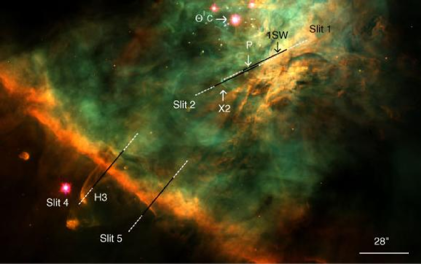
The observations of NGC 1976 described here were taken as part of our HST Cycle 7 program GO-7514. We observed with 4 different STIS long-slits: slits 1, 2, 4, and 5. These are shown in Figure 1. Our slit positions are chosen to cross several features, including an Herbig-Haro (HH) object, a proplyd, and the Orion Bar. Slit 1 passes through the position 1SW which we observed with FOS and GHRS in Cycle 5 (see Figure 1 in Rubin et al. 1997). The centre of 1SW is at , = , 23′415 (all positions are equinox J2000), 18.5′′ S and 26.2′′ W of Ori C. This slit was also chosen to pass through proplyd P159-350 (O’Dell & Wen 1994). Slit 2 passes through position x2 observed with FOS in Cycle 5 (see Figure 1 in Rubin et al. 1997). x2 is located in one of the most prominent arcs in the [O III] WFPC2 images. Slit 2 is parallel to slit 1, which allowed a substantial saving in overhead (OH). The position angle (PA) = 114.555o; the distance between slit centres is 18.1′′. Note that the bottom of slit 1 and the top of slit 2 have a separation of only 0.211′′. The displacement between these two slits in the direction along the slit is 18.056′′.
Slit 4 crosses the Orion Bar and is oriented to point toward Ori C (the dominant exciting star), which also places it essentially orthogonal to the Bar. The southern tip passes through the Herbig-Haro object HH 203. Slit 5 passes through a very bright, sharply-defined “rim” of the Bar where a positional bifurcation begins. Slit 5 is parallel to slit 4 in order to take advantage of the same OH savings as is the case for slits 1 and 2. The PA = 139.068o; distance between centres of slits 4 and 5 is 32′′.
Observations were made as follows: data for slits 1 and 2 are from Visit 2 (1998 December 7 UT), Visit 52 (2000 December 7) and Visit 72 (2001 December 16); data for slits 4 and 5 are from Visit 5 (1998 December 22). All our data described here were acquired using the STIS/CCD with a 52′′ slit length and 0.5′′ slit width. Each visit comprises 2 orbits. Spectra were taken with gratings G430M (with wavelength settings: 3680, 4451, 4961) and G750M (settings: 5734, 6581). Each exposure was done in accumulation mode and at least two spectra were taken at each setting in order to cosmic-ray (CR) clean. The data sets we processed were those obtained after sufficient time elapsed from the observation dates in order that “best reference files” would be stable/finalized. We requested On-the-Fly Calibration for science files and Best Reference Files. After retrieving the data sets, we then co-added and cosmic ray cleaned images using standard packages in IRAF.111IRAF is distributed by NOAO, which is operated by AURA, under cooperative agreement with NSF. Calibrations to produce 2-dimensional (2D) rectified images were then carried out. From these, we singled out specific emission lines for further investigation. Data for the [O III] 4364 Å line as well as H 4342 Å were contained in the G430M/4451 grating setting; for the [O III] 5008, 4960 Å lines and H 4863 Å lines, G430M/4961 was used; for [N II] 5756 Å, G750M/5734 was used; for H 6565 Å and the [N II] 6550, 6585 Å lines, G750M/6581 was used. All wavelengths in this paper are vacuum rest wavelengths.
For G430M, the dispersion is 0.28 Å per pixel for a point source and the plate scale 0.05 arcsec/pixel (Leitherer et al. 2001, Chapter 13). For a uniformly filled slit with width 0.5′′, a degradation in resolving power by a factor of 10 is expected to a spectral resolution of 2.8 Å. For G750M, the dispersion is 0.56 Å per pixel for a point source and the plate scale 0.05 arcsec/pixel. For a uniformly filled slit with width 0.5′′, the spectral resolution would be 5.6 Å.
According to Paul Goudfrooij (private communication), the STIS CCD absolute flux calibration that is performed in the pipeline follows methods described in Instrument Science Report (ISR) 97-14 (Bohlin, Collins & Gonnella 1998) available through the STIS web site at www.stsci.edu/hst/stis/documents/isrs. That report considers only the L (low-resolution) modes specifically, but the flux calibration for the M (medium-resolution) modes is done the same way, i.e., by comparing the observed spectrum of a primary standard with a pure-hydrogen white dwarf model. The calibration observations were made with the 52′′2′′ slit; thus relative transmission corrections are necessary to derive the absolute fluxes for the other slits (such as the 52′′0.5′′ slit we used). This procedure is documented in ISR 98-20 (Bohlin & Hartig 1998).
For the analysis presented here, we were interested mainly in the distribution of line flux along the slit spatial direction. This was accomplished with the IRAF routine blkavg in conjunction with specialized software tools that we developed ourselves. Even after applying the standard CR rejection there still remain many bad pixels due to CRs and/or hot pixels. There is considerable danger that including these can corrupt the flux values we seek. The program developed to eliminate these remaining bad pixels is called PIXHUNTER, which has been described briefly in an earlier paper (see Appendix A of Paper I). Once the columns containing the line have been cleaned for deviant pixels, we are ready to subtract an equivalent spectral range of continuum. We do this by using IRAF functions, including blkavg, to operate upon the appropriate sections of cleaned continuum. The 1-dimensional (1D) distribution of line flux versus spatial coordinate for the various emission lines of interest is what we need for our subsequent physical analysis.
We note that there is excellent agreement with a cross check of the 1D results of flux versus spatial direction by comparing with 1D results of flux versus wavelength for a corresponding spatial sample. The latter were measured with the splot package. With this, the underlying continuum is fitted and the integrated line flux determined with the -option (area under the line profile), which was preferable to fitting with a Gaussian profile. Because of the spectral impurity introduced by the relatively wide slit used, the line profiles have flatter tops and less extended bases (i.e., they are more “trapezoidal”) than the Gaussian fits. It is also apparent that the Gaussian fit is overestimating the line flux.
Both the [O III] 5008 and 4960 Å lines were observed simultaneously with theG430M/4961 grating setting. Because both transitions arise from the same upper level, the intrinsic flux ratio depends only on the transition probabilities (A-values) and wavelengths. As reported previously for similar STIS observations of the planetary nebula NGC 7009 obtained under program GO-8114 (PI RR) (Paper I), what we found was a surprising variation in the F(5008)/F(4960) ratio with position along the slit. This amounts to a variation in the ratio of roughly 3.00.1. Furthermore, it appears more-or-less periodic with an 3.5′′ cycle. As described in Paper I, according to Ted Gull (private communication), this is an instrumental effect and is a ratio of two fringe patterns. The source of the problem is a thin blocker filter that had to be matched with each grating and the best (and only) location that it could be placed was above the grating in a stable mounting. To attempt to do anything about fringing would probably require a dedicated HST/STIS calibration program. If there were fringing in the F(5008)/F(4364) ratio at the same level as for the F(5008)/F(4960) ratio, the 3.3% error would result in only a minor error, e.g., 100 K at = 104 K (see §4.1).
3 EXTINCTION and REDDENING CORRECTION
Before deriving the distribution from the STIS data, we first correct for extinction. This is calculated by comparing the observed F(H)/F(H) ratio with the theoretical ratio I(H)/I(H). We use a value of 2.88 assuming = 8500 K and = 5000 cm-3, Case B (Storey & Hummer 1995).222For conditions applicable to NGC 1976, we find using an online program (see Storey & Hummer 1995) that the I(H)/I(H) ratio used here will depart by less than 3% over the range 7500 12500 K and 103 105 cm-3. The extinction correction is done in terms of (H), given by the relationship
| (1) |
where ) is the extinction curve. For the H (4342), 4364, 4863, 4960, 5008, 5756, 6550, 6565, and 6585 Å lines, the respective values for ) are 0.0856, 0.082, 0, 0.0153, 0.0225, 0.1237, 0.2185, 0.2202, and 0.2226, (Martin et al. 1996). This leads to,
| (2) |
The correction for extinction/reddening from observed to intrinsic flux for the 4364 and 5008 lines is then given by,
| (3) |
and for the 5756 and 6585 lines by,
| (4) |
For the STIS data, we binned the pixels along the slit into tiles that are 0.5′′ square (matching the slit width). The STIS fiducial bars are excluded. This produced (H) results for from 79 to 96 tiles, depending on the slit/visit observed, which are the same set used later for the analysis. The distributions of (H) along the two slits (slit 1 and slit 2) observed in 3 separate visits (V2, V52, and V72) are remarkably similar. Furthermore, the distributions match well for the regions of slit 1 and slit 2 that are adjacent to each other. Recall that the separation between the bottom of slit 1 and the top of slit 2 is a mere 0.211′′ and that slit 2 is shifted 18.056′′ relative to slit 1 along the slit spatial direction. The average (H) values without regard to any weighting for brightness are: for slit 1: 0.680, 0.699, and 0.701 respectively for the three visits; for slit 2: 0.762, 0.798, and 0.766. For slit 4, it is 0.566 and for slit 5, it is 0.611. We comment further on slit 1, which covers the proplyd P159-350 and 1SW. Starting at the SE end of slit 1, the values are roughly flat at 0.85. There is a spike to 1.43 in V2 at the tile containing most of the proplyd. The behavior is similar for V72 with a spike to 1.33 at the tile containing most of the proplyd. The adjacent nebula has for both visits a (H) value of 0.9. Unfortunately, because P159-350 was centred in the East fiducial bar on V52, we cannot reliably measure (H) there. Where slit 1 crosses 1SW, (H) is 0.6, which agrees well with our previous spectroscopic value 0.605 at our position observed with the Faint Object Spectrograph (FOS-1SW, Rubin et al. 1998). At the end of slit 1 toward the NW, (H) has decreased to 0.4.
We examined the vicinity of P159-350 in more detail using the original resolution of 1 pixel (0.05′′) for slit 1 in the spatial direction. The increase in flux and thus signal-to-noise (S/N) in the vicinity of the proplyd permits meaningful analysis here. For V2, we find that the peak observed flux occurs in pixel 311 for the H (5.6410-11 erg cm-2 s-1 arcsec-2) H (6.8310-12), and 4364 (3.1810-13) lines, while the 5008 line reaches the highest peak (6.7110-12) at pixel 317 and a second relative maximum (5.1410-12) at pixel 305 with a clear trough between these, having a relative minimum (3.5810-12) occurring at pixel 310. The F(H)/F(H) ratio peaks at 8.269 also at pixel 311 and hence the derived (H) reaches a peak value there of 2.08.
Repeating the analysis for V72, we find that the peak observed flux occurs in pixel 343 for the H (2.1910-11) and 4364 (8.1110-14) lines. The H peaks in pixel 344 (3.1910-12) and is lower at pixel 343 (2.7410-12). The 5008 line reaches the highest peak (5.7710-12) at pixel 350 and a second relative maximum (4.5810-12) at pixel 336, again with a distinct trough between these, having a relative minimum (2.8510-12) occurring at pixel 344. The F(H)/F(H) ratio peaks at 7.994 at pixel 343 where the derived (H) reaches a peak value of 2.01. The fact that the peak surface brightnesses are much higher for P159-350 in V2 compared with V72 is most likely because the brightest part of the proplyd was better sampled and/or aligned with the 1 pixel 10 pixel (0.05′′ by 0.5′′) “smallest rectangular aperture” in the former visit than the latter.
4 ELECTRON TEMPERATURE DETERMINATION
4.1 [O III] Electron Temperature
The electron temperature is derived from the intrinsic ratio I(5008)/I(4364) using the following relation,
| (5) |
Effective collision strengths are from Burke, Lennon & Seaton (1989) for = 104 K. Transition probabilities (A-values) are from Froese Fischer & Saha (1985). Note that this holds in the low- limit, which should be valid for Orion where values are less than the critical densities () for these lines. The lowest 6.4105 cm-3 for the 5008 line, which is well above values determined (e.g., Peimbert & Torres-Peimbert 1977; Osterbrock, Tran & Veilleux 1992; Esteban et al. 1998).
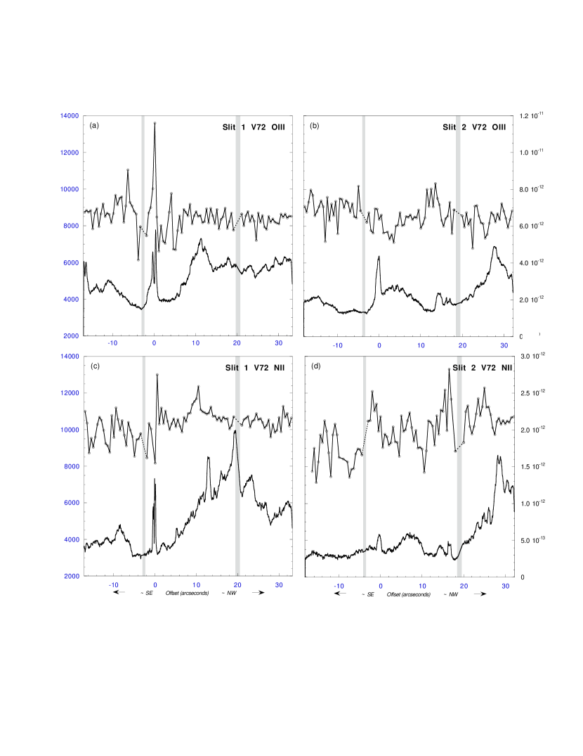
We continue with the analysis using the tiles along the slit described above; the number of usable tiles varies with the slit/visit and ranges from 79 to 96. Equations (2), (3), and (5) are applied to the four emission lines to derive . Figure 2(a) shows the distribution of versus position along slit 1. For slit 1, position along the slit is relative to the location of peak surface brightness (S.B.) in the H line, which occurs at P159-350. We set our zero corresponding to coordinates, , = , 23′5004 (Bob O’Dell, private communication). As mentioned in the last section, there is actually a relative minimum in the [O III] 5008 Å S.B. close to that position. The lower curve in Figure 2(a) shows the observed 5008 S.B. (erg cm-2 s-1 arcsec-2), which is displayed (unsmoothed) at the pixel level providing 0.05′′ spatial resolution along the slit. The feature at the very left (SE) end of this slit is associated with the prominent arc, part of which we used to define our position x2 and which was better observed in slit 2. The open circles on the top () curve represent the individual tiles plotted at their midpoint. The dashed lines are a linear interpolation across the tiles that were deemed to have unreliable measurements because of proximity to the fiducial bars. There is a remarkably flat distribution with the notable exception of an upward spike to 13600 K at the tile containing the bulk of the proplyd H emission. For slit 1 and V2, the behavior is similar with a sharp upward spike to 15050 K at the tile containing the bulk of the proplyd H emission. It is most unlikely that these high temperatures are realistic (these tiles are omitted in the statistical analysis to follow) and are the result of equation (5) not accounting for the higher electron densities, probably in excess of 106 cm-3, in P159-350. Because the 5008 line will then suffer considerable collisional deexcitation, derived using equation (5) will be overestimated (e.g., Viegas & Clegg 1994). In the next section, we will evaluate the distribution of along slit 1, as well as along the other slits, in terms of variations.
Figure 2(b) shows the distribution of versus position along slit 2, where position along the slit is relative to the location of the local peak S.B. in the 5008 line that occurs at x2. Using the position of P159-350 and the specified offset from slit 1 to slit 2 of 1.08s in RA and 8.15′′ in Dec., we find x2 coordinates: , = , 23′5773. The lower relative maximum near offset +14′′ is where slit 2 passes through the “downstream” tail of P159-350. Again there is a remarkably flat distribution.
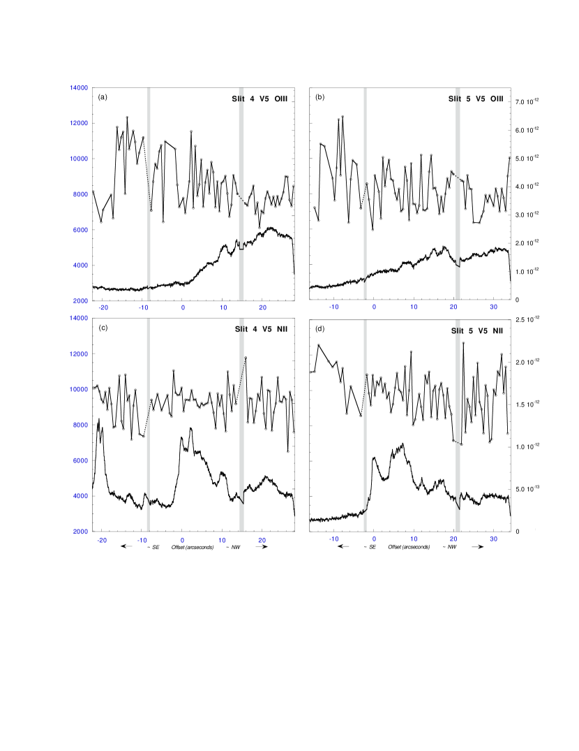
Figure 3(a) plots the distribution of versus position along slit 4, where position along the slit is relative to the location of a feature in the bar seen in the 6585 S.B. distribution (Fig. 3(c)) discussed in the next section. Recall that this slit is aligned to point toward Ori C. While there is an underlying decrease in the 5008 S.B. with increasing distance from Ori C, there is a leveling off (plateau) at the SE end of slit 4 of 5008 emission that remains substantial well beyond the bar. This is consistent with the WFPC2 images of the region; the composite “drizzled” image by Walsh (1998) that includes filter F502N (which covers the 5008 line) depicted in green, shows a green hue in a parabolic shape that appears to be a wake emanating from HH 203 and HH 204. Walsh’s image is available at stecf.org/newsletter/webnews1/orion/m42col_drizzle.jpg. The point was also made in an earlier discussion of HH 203 and HH 204 (O’Dell et al. 1997). Along this slit, the distribution is also fairly flat, especially in the region of higher S/N (see §4.2). There is a clear increase in the amplitude of the fluctuations for the tiles SE of the bar due to poorer S/N in the 4364 Å line.
In Figure 3(b), we plot the distribution of versus position along slit 5. Here, the position along the slit is relative to the location of a feature seen in the 6585 S.B. distribution (Fig. 3(d)) discussed below. There is roughly a linear decrease in 5008 emission from the NW to the SE end of slit 5 with a “jump” occurring between 18–22′′ offset position. As was the case for slit 4, here too there remains substantial 5008 emission beyond the bar that is evident in the green hue at this location in the Walsh image. The distribution here is flat similar to that for slit 4; the increase in the amplitude range at the SE end of the slit is again due to poorer S/N in the 4364 Å line.
4.2 [N II] Electron Temperature
The in the N+ zone is derived from the intrinsic ratio I(6585)/I(5756) (see equations (2) and (4)). Because the critical density for the 6585 line, 7.7104 cm-3 (at 104 K), is substantially less than for the [O III] 5008 line (6.4105 cm-3), we do consider various values when deriving . We also derive temperatures utilizing two different sets of N II effective collision strengths – those calculated by Lennon & Burke (1994) and by Stafford et al. (1994). We use the effective collision strengths for 10000 K; these do not vary much with the range of interest in Orion. The A-values used are discussed in Rubin et al. (1998, Appendix A with original references therein).
For non-zero densities, our derivation of is done in an iterative fashion, starting with an initial estimate in the low- limit. Then the volume emissivities ( values) for both the 5756 and 6585 lines are calculated solving the statistical equilibrium equations for the six lowest energy levels. The value is then recomputed using the intrinsic ratio I(6585)/I(5756), (6585), and (5756). The rapidly converging iteration is halted when changes by less than 1 K.
In this paper, we are interested in assessing the amount of that can occur. Thus, we limit our analysis here by not including a detailed study of density variations, which is the subject of future papers by the present authors. Nevertheless, it is necessary to include some discussion of with regard to deriving the [N II] . As is well known, there is an inverse scaling of [N II] with . First we perform the calculations for in the low- limit. This provides a firm upper limit to the distributions evaluated for the various slit/visit data. We also repeat the full computations for 4 other ’s: 1000, 2000, 5000, and 10000 cm-3. The last value is more than high enough to bracket expectations for Orion, with the exception of objects like the proplyds as will be discussed below for P159-350. The value of 5000 is our best single to cover the region of slits 1 and 2 (e.g., Pogge, Owen & Atwood 1992). Their map of the electron density in the S+ zone indicates that is lower in the regions of our slit 4 and slit 5; for these, we adopt a best single = 2000. It is these respective densities that are used to depict the distribution along slits 1, 2, 4, and 5 of [N II] in Figure 2(c), 2(d), 3(c), and 3(d) respectively. For the Figures, we have used the N+ collision strengths of Lennon & Burke (1994) while results from this set, as well as Stafford et al. (1994) will be tabulated later. The lower curve in each of these panels shows the 6585 surface brightness distribution along the slit.
Figure 2(c) shows the tiled [N II] distribution versus position along slit 1 and is a positional match to Figure 2(a). The lower curve here shows the observed 6585 Å S.B. at the unsmoothed pixel level. There again appears to be a relative minimum in the [N II] 6585 S.B. at the centre pixel for P159-350 although it is not as well defined as the dip in the 5008 S.B. there. As with the 5008 curve, the peak S.B. on the NW side of the proplyd exceeds that on the SE side. However, the overall 6585 emission is much narrower in P159-350 than is the 5008 emission. In totality, the structural behavior in the 6585 emission compared with that in 5008 is consistent with the N+ region being more tightly confined than is the O++ region to the low-mass star of P159-350, which is expected if the proplyd is externally ionized by Ori C. The prominent absolute maximum of the 6585 S.B. is very close to the 1SW position, 20.26′′ from P159-350, which is somewhat blocked by the NW-side fiducial bar. The narrow secondary peak at 13′′ offset appears to be associated with the much broader secondary maximum near offset 12′′ in the 5008 S.B. of Figure 2(a). There is perhaps an ionization boundary being observed here, although the slit orientation is far from ideal to test this. A slit pointing toward Ori C would be better suited. Once again, there is a notably flat distribution with the exception of the proplyd. In Figure 2(c), we have omitted the tile with the highest derived of 20815 K. The highest in the plot is at 13000 K. Both these tiles are omitted from the subsequent statistical analysis. These high derived ’s are undoubtedly pointing more to high values associated with the proplyd than high temperatures. The assumed for the calculation of in Figure 3(c) is 5000 cm-3, while for P159-350 may exceed 106 cm-3. Because the 6585 line emission will suffer enormously from collisional deexcitation at more realistic densities, the derived would be much lower. For slit 1, V2, there are two tiles at the proplyd that have an enormous upward spike in to 29800 and 35850 K; both tiles are omitted from the statistical analysis in following sections.
Figure 2(d) has the distribution of [N II] versus position along slit 2. There is a fairly flat distribution with some indication of a drop in SE of the lower fiducial bar. The maximum 6585 S.B. in the lower curve occurs near offset 28′′. This location is immediately adjacent to the narrow peak at 13′′ offset in Figure 2(c), just mentioned. The relatively small peak at x2 (offset 0) further supports the finding in the WFPC2 composite image that the emission arc which includes the position x2 is mainly an [O III] feature (see Figure 1). We note that x2 is part of the HH 529 complex and more specifically, the easternmost feature called 170-358 (see fig. 20 in Bally, O’Dell, & McCaughrean 2000). According to their study, including the kinematics, 170-358 is an expanding bow shock seen from the side.
Figure 3(c) plots the distribution of [N II] versus position along slit 4. Position along this slit is relative to the location of the SE-most peak in S.B. in the 6585 line. We set our zero corresponding to coordinates: , = , 24′4821 determined from the position of our offset star Ori A (HD37041) with , = , 24′579. There is a brighter feature that occurs where the slit crosses HH 203 at offset near . Comparison with Figure 3(a) shows no enhancement in 5008. This is consistent with the WFPC2 images of the region; the composite image in Figure 1 that includes filter F658N (isolating the 6585 line) shows HH 203 as a reddish-orange object. There is a very flat distribution even over the wide range of S.B. and ionization structure along slit 4.
In Figure 3(d), we plot the distribution of versus position along slit 5. Here, the zero position along the slit is the SE-most 6585 S.B. peak of where there is a bifurcation in the bar (see Figure 1). This feature appears to mark the boundary between the ionized region and the photodissociation region (PDR). Using the position of Ori A and the specified offset from slit 4 to slit 5 of s in RA and in Dec., we find: , = , 25′0814. Beyond this position, the distribution becomes less reliable because of poorer S/N in the 5756 Å line. Overall, the is flat as has been the case throughout.
5 FRACTIONAL MEAN-SQUARE TEMPERATURE VARIATIONS
Our STIS analysis above presents results in the plane of the sky. The observations here do not address temperature fluctuation along the line of sight, which may be characterized in terms of the average temperature and fractional mean-square variation () as defined by Peimbert (1967).
| (6) |
| (7) |
where is the ion density ) or ). The integration in equations (6) and (7) is over the column defined by each tile, and along the line-of-sight (). We are unable to measure the along the for any column (cross section 1 tile). If there are along the , we can say that or (e.g., Peimbert 1967; Rubin et al. 1998).
In the case of [O III], for each tile, we have calculated . Then the intrinsic flux I(5008), fully correcting F(5008) for extinction (see equ. 3), in each tile is used in conjunction with = for that tile, and assumed constant along the , to derive the following:
| (8) |
Here is the excitation energy above the ground state for the upper level of the 5008 transition, k is Boltzmann’s constant, is known from atomic data, and has finally incorporated the known factor with the atomic constants. Here we again make the safe assumption of the low-Ne limit (negligible collisional deexcitation) discussed earlier.
For the case of [N II], for each tile, we have calculated . Then the intrinsic flux I(6585), fully correcting F(6585) for extinction (see equ. 4), in each tile is used in conjunction with = for that tile and the chosen value for , and assumed constant along the , in the following relation:
| (9) |
Here is the normalized volume emissivity which is related to the usual volume emissivity by /(). depends on the (fractional) population in a given level obtained by solving the 6-level atom for the specific and . It is not necessary to deal with the constant of proportionality for our purposes.
Following Paper I, we define the average () and fractional mean-square variation () in the plane of the sky.
| (10) |
| (11) |
where represents an element of surface area in the plane of the sky and the integration over is for each tile along the . The proper weighting for each tile is provided by either equation (8) or equation (9) depending on whether we are performing an [O III] or [N II] analysis.
The results using the STIS data for the various slits and visits to determine and are summarized in Table 1. These quantities for [O III] are entered in the first column. For slit 1, Visit 72 (see Figure 2(a)), = 8258 K and = 0.00925. We have excluded the spike in at the proplyd. The value for is remarkably low, although not as low as the value of 0.0035 that we found for NGC 7009 (Paper I). The results from the other visits (V2 and V52) for slit 1 are close to those for V72. Our results for slit 2 and all three of the visits show values in close accord and similar to those for slit 1. All these averages vary by less than 285 K. By comparing for slits 1 and 2 in all 3 visits, we see that all six numbers are small, ranging from 0.00682 to 0.0129. For slits 4 and 5 the statistics are roughly comparable and differ from those for slits 1 and 2 in the following ways: is several hundred K smaller and is somewhat higher, although the largest value, 0.0176, is still notably small. A simple visual comparison of the plots in Figs. 2(a), 2(b), 3(a), and 3(b) leads one to conclude that looks larger for slits 4 and 5, particularly with the larger excursions in the regions SE of the bar. We note however that these data with poorer S/N have a minor effect on the statistics. There is natural biasing against these tiles due to weaker emission in both 4364 and 5008 as can be seen from equation (8), which in turn provides a smaller ()–weighting of these tiles in equations (10) and (11).
All the remaining columns in Table 1 pertain to the derivation of and for [N II]. These are displayed for 5 different electron densities and two different sets of effective collision strengths. As described, for slits 1 and 2, our preferred is 5000 cm-3, while for slits 4 and 5, it is 2000 cm-3. We will now discuss the resulting numbers in these particular density columns and also using the left-side column with the Lennon & Burke (1994) collision strengths, unless stated otherwise. For slit 1, Visit 72 (see Figure 2(c)), = 10226 K and = 0.00695. We exclude the high near P159-350 (see §4.2). The value for is even lower than found for this slit/visit in the [O III] analysis; is nearly 2000 K higher. There is close agreement among the N+ and values for all the visits for slit 1; the above intercomparison between N+ and O++ with the corresponding numbers in the respective visits is also true.
For slit 2, the numbers vary by more than 400 K between visits; the respective ’s are smaller than for slit 1 for V52 and V72 but slightly higher for V2. All of the values are larger for slit 2 than for slit 1, reaching 0.0146.
For slits 4 and 5, the N+ is several hundred to more than 1000 K smaller than for slits 1 and 2. Compared with the O++ , slits 4 and 5 are higher by 1343 and 1749 K, respectively. at 0.0175 is largest for slit 5 and nearly identical to the corresponding O++ value, which is also the highest in the first column. This larger may be attributed to the larger excursions in in those tiles SE of the bar, where the S/N in the 5756 Å line is poorer. A comparison of Figure 3(c) and 3(d) clearly indicates a much lower 6585 S.B. SE of the bar for slit 5 than for slit 4. Again we emphasize that these data with poorer S/N play only a minor role in contributing to the integrals in equations (10) and (11). When there is weaker emission in both 5756 and 6585, as can be seen from equation (9), there is a smaller ()–weighting of these tiles in equations (10) and (11).
The effect of substituting the Stafford et al. (1994) collision strengths is small for both slit 1 and slit 2 for all 3 visits: decreases by less than 200 K; decreases by roughly 5–6 percent. The drop for slits 4 and 5 is slightly more, up to a 276 K difference; decreases by 6–7 percent.
On the whole, the results presented in Table 1 allow us to reach two robust conclusions. First, is always very small ( 0.0182) for either the O++ or N+ analyses. Second, the derived from the [O III] lines is always significantly less than derived from the [N II] lines. These hold even when we consider for the N+ analysis a wide range in that should amply bracket the great bulk of the plasma in Orion and also examine the influence of using alternative collision strengths.
In Appendix A, we present an analysis of the uncertainties in the derived values as well as the values.
6 DISCUSSION AND CONCLUSIONS
We extend our earlier study of electron temperature variations from the [O III] (4364/5008) flux ratio in the PN NGC 7009 (Paper I) to the Orion Nebula. In addition, we use our STIS long-slit observations to expand the analysis to measure variations from the [N II] (5756/6585) flux ratio. The observations here do not address fluctuation along the line of sight through the specific O++ region or, likewise, through the N+ region. We analyse both the [O III] and [N II] data sets to derive the average and fractional mean-square variations in the plane-of-the-sky, which we call and . We assume for each square column (projection of 1 STIS tile 0.5′′ square on the plane-of-the-sky) that the plasma along the line of sight is isothermal at the in the case of O++ or in the case of N+. For the latter case, we consider a large range of values, which should be sufficient for Orion, in order to produce Table 1. The analysis for each assumes that it is constant for the entire STIS slit length and throughout the sheet projected through the nebula along the .
Fluctuations in (and ) along the are inevitable. We can make some comments about how our results for might be adjusted by variations along the . The relationship between and for the O++ region is
| (12) |
and between and for the N+ region is
| (13) |
(e.g., Peimbert 1967; Rubin 1969). With the – or –values for Orion (see Figures 2 and 3) or indeed for H II regions in general, will be smaller than these temperatures inferred from the forbidden line flux ratios here. Rather than repeat some examples of how the differences depend on , the reader is referred to our comments in the earlier paper (§7 in Paper I).
We do not have the data here to characterize variations in 3-dimensions (3-D). It is useful to define an overall 3-D average () and fractional mean-square variation (). These single values apply for the entire source. Equations (6) and (7) define these specific values when the integration is over the entire volume. We note that for a spatially unresolved object (total integrated fluxes observed in the aperture), not the case for Orion, = and a calculation of is meaningless.
Our measurements of reported here are an average along each line of sight. Because each element of area treated in the plane of the sky represents a column which has already created a spatially averaged temperature along the (e.g., see fig. 1 in Rubin 1969), it is likely that the value for is substantially higher than . Measurements of along various sight lines appear to be the most direct way to reliably gauge . Therefore, despite finding remarkably low , we cannot completely rule out much larger temperature fluctuations along the . Further work, beyond the scope of this paper, is underway that will use modeling as well as additional observational data in an effort to better determine the relationship between , , and .
Finding [N II] temperatures that are higher than [O III] temperatures is not a new result. For Orion, this has been known for years (e.g., Baldwin et al. 1991). What is new/significant here is that we have results from many more sight lines, more than 700 represented by the individual tiles, with improved spatial resolution (0.5 arcsec squares) and excellent spatial registration between the [N II] and [O III] data sets that HST affords. Of the roughly 700 tiles, about half represent independent sight lines, with the other half having spatial overlap due to the repeated visits for slits 1 and 2.
The fact that the [N II] temperatures are higher is also expected on theoretical grounds and again, not something novel that we have uncovered. We enumerate three factors that contribute to the predicted inequality. First, the cooling of the [O III] 5008, 4960 Å lines in the O++ region is uniquely efficient for nebular conditions and elemental abundances that prevail in Galactic H II regions, including Orion. On the other hand, in the “singly ionized” region (where the dominant O and N ions are O+, N+) there is no coolant that is nearly as efficient as [O III] 5008, 4960 is in the O++ zone. Additionally for Orion, the blister geometry likely results in higher average electron densities in the singly ionized region compared with the O++ region because the former is closer to the PDR. The higher in the N+ region would also contribute to less efficient cooling.
Second, there is the predicted hardening of the stellar ionizing photons at progressively larger distances from the exciting star. This is due to the functional form of the H photoionization (predominantly) cross section, which diminishes steeply with higher frequency from its value near threshold. At larger distances from the exciting source, the average energy per photoionization will increase and thus the heating rate will also increase. This causes a rise in with an increase in distance (other factors being equal). This has been known for many years (e.g., Rubin 1968).
Third, there is a possibility that there is a contribution to the production of [N II] 5756 Å emission (and to a lesser extent 6585) by recombination and cascading. Under some conditions, this may provide significant routes into the upper energy level of the 5756 transition that are not negligible compared with collisional processes. This was examined by Rubin (1986). If there were a significant “recombination” contribution to the observed emission, we would have overestimated the derived from the [N II] 5756/6585 flux ratio. With our two independent, detailed models for the Orion Nebula (Baldwin et al. 1991 and Rubin et al. 1991), the recombination contribution appears to be small. We discussed this in a subsequent paper where these models were “retrofitted” with more in-common input parameters, including the Stafford et al. (1994) N+ collision strengths, to allow closer intercomparisons (see end of §4 in Rubin et al. 1998).
All three of the above effects are included in our photoionization, plasma simulation models just mentioned. The predicted [N II] and [O III] temperatures for the entire volume are 8721 K and 7704 K in the Rubin et al. (1991) model and 8649 K and 7692 K in the retrofit (Rubin et al. 1998) using Stafford et al. cross sections. When the Lennon & Burke (1994) N+ collision strengths are used instead of the Stafford et al. set, the respective temperatures become 8706 K and 7701 K.
Finally, we encapsulate the findings here for the proplyd P159-350. We find large local extinction as evidenced by the dramatic increase in the observed F(H)/F(H) ratio along slit 1. For V2, this ratio peaks at 8.27 which implies a (H) of 2.08 from the Balmer decrement. Similar values are found for our V72 observations: F(H)/F(H) peaks sharply at the proplyd position reaching a ratio of 7.99, where the derived (H) = 2.01. Because the adjacent nebular values for (H) are much lower, the extinction must be associated with the P159-350 environs.
A comparison of the [O III] 5008 and [N II] 6585 surface brightnesses in the vicinity of P159-350 (see Figures 2(a) and 2(c)) shows for both lines that the S.B. on the NW side of the proplyd exceeds that on the SE side. However, the 6585 emission is much narrower than is the 5008 emission which provides evidence of ionization stratification consistent with the N+ region being more tightly confined than is the O++ region to the low-mass star of P159-350. This “inverse H II region” behavior is precisely what is expected due to the external ionization source Ori C.
The derived distributions were all notably flat except at the position of the proplyd observed in slit 1. The very high derived ’s at the location of P159-350 are no doubt due more to high values associated with the proplyd than high temperatures. As stated, the calculations used here to assess have not accounted for values likely to exceed 106 cm-3 in P159-350. Because both the 5008 line and even more so the 6585 line emission will suffer substantial collisional deexcitation at such high densities, the derived for both [O III] and [N II] would be much lower.
Each of the above mentioned facets of P159-350 deserves further study. The smallest spatial resolution element was 1 pixel (0.05′′) in the spatial direction by 10 pixels (0.5′′) in the dispersion direction. It would be highly desirable to obtain higher spatial resolution of P159-350, which can be readily achieved by observing with a narrower STIS slit. The narrower slit would enable better spectral resolution as well and permit a detailed mapping of P159-350 in the C III] 1907, 1909 Å lines. The ratio of their fluxes is an excellent diagnostic of even at the high values expected in proplyds. Improved spectral resolution in the optical lines will also help sort out kinematics from spatial structure, which was a difficulty with the 0.5′′ slit width we used.
Appendix A Error Analysis
The values found for are very small. It is important to determine whether even these small fluctuations in from tile to tile are a real signal or the result of measurement uncertainty.
From equation (5) for O++, it can be shown that the mean square uncertainty in temperature, expressed as , has the following dependence on the uncertainties and of the nebular () and auroral () line fluxes, respectively:
| (A1) |
where . We use this as an approximation for N+ too, with .
The uncertainty is principally the measurement error in the line flux for a tile. The S/N for the flux of the auroral lines ([O III] 4364 and [N II] 5756 here) is much lower than that for the nebular lines ([O III] 5008 and [N II] 6585 here), and so the uncertainty of the weaker auroral line will dominate the uncertainty . The uncertainty also depends on the (differential) extinction correction, but in the present case this is a small effect compared to the uncertainty in the observed auroral line fluxes (hence, S/N ).
The three independent methods used to calculate the S/N of the auroral lines are discussed in the following sections. We use to calculate the corresponding .
A.1 Method 1
The flux integrated over the line profile as found using the “blkavg sum” technique in IRAF is
| (A2) |
where is the monochromatic flux for the tile (erg cm-2 s-1 Å-1), is the dispersion conversion (Å/pixel), is the number of pixels in the spectrum used to define the and is the number of pixels used for the . Since the auroral line is weak, the rms fluctuation in the can be assumed to be the same as in the , . Thus, the rms of the line flux is
| (A3) |
In our measurements we used . The above three equations are used to create the entries for method 1 (M1) in Table 2. Values are given for both the [O III] 4364 and [N II] 5756 lines for all slits (for slits with multiple visits, a representative case is given).
A.2 Method 2
In this method, the line profiles from the STIS spectra are fit with a template (a Gaussian convolved with a slit of width 0.5″) using a combined Gauss-Newton and modified Newton algorithm (Numerical Algorithms Group (NAG) - E04FDF) to find the minimum least-squares solution and the corresponding variances of the variables used in the fit (NAG-E04YCF). The slit width is held constant, but due to anamorphic magnification in the dispersion direction, the plate scale differs from line to line which results in different slit widths expressed as pixels (see Bowers & Baum 1998).
The variables used in the template fitting are the flux , the FWHM and central wavelength of the Gaussian, and the slope and mean brightness of the continuum. The variances reflect how well the model fits the data. Keeping all of these as variables gives one a conservative estimate of the variance of each. Note that a poor template would lead to an overestimate of the error. The templates were tested on the strong nebular lines and generally fit very well. However, there are instances where the surface brightness changes across the slit (in the dispersion direction), so that the implicit assumption of uniform illumination is not perfect. Therefore, the estimated uncertainty from method 2 is an upper limit. As is seen in Table 2 it agrees well with the error estimated using method 1.
A.3 Method 3
This method utilizes the multiple sets of observations for slit 1 and slit 2 in the three visits V2, V52 and V72 and examines the reproducibility of the line fluxes and . There are adequate fiducial sources visible in all three visits so that the spectra may be shifted in the spatial direction to achieve alignment to 1 pixel. The proplyd P159-350 in slit 1 is particularly useful for this and serves for slit 2 as well because the relative positional HST offsets between slit 1 and slit 2 are not subject to the acquisition uncertainty. There is also positional alignment uncertainty in the dispersion direction which is more difficult to estimate. For all three visits, P159-350 was seen in the 0.5′′ wide slit; although it was blocked for the most part by the East fiducial bar in V52, some of the emission still peeks out both ends. We noted at the end of section 3 that P159-350 has a higher peak surface brightness in V2 than in V72. We estimate that the positional alignment of the tiles perpendicular to the spatial direction between the three visits is within 0.2′′ so that there is substantial area overlap (perhaps 60%) of our tiles between the three visits. Comparison of the nebular line strengths from visit to visit shows excellent reproducibility ( per tile for the O++ line). This is much smaller than the auroral line differences found among successive visits. The measurement error of the weaker auroral lines is of course higher. Furthermore lack of registration is a more serious issue for the auroral lines (from a much higher energy level) if there are real fluctuations on this spatial scale; in the limit of no overlap, one would expect even if there were no measurement errors. Therefore, having from method 3 larger than from M1 and M2 is not unexpected.
For each tile in common between V2, V52 and V72, both an average value () and the standard deviation () of any single determination of were calculated. The representative value entered as M3a in Table 2 is the median for each of the slits; as in methods 1 and 2, the listed is what is implied by this S/N, through equation A1.
For each in-common tile, we also calculated for each visit, then the average and the actual standard deviation () of any single determination of . The median for each slit is included in Table 2 as M3b. From these median values we calculated the tabulated . Methods 3a and 3b agree closely, as they should given the good reproducibility of the nebular lines (i.e., the effect of in equation A1 is negligible).
The analysis summarized in Table 2 shows that the measured is a real signal not dominated by the noise and/or measurement errors. The two exceptions are for the O++ measurements for slits 4 and 5 which include tiles beyond the Orion bar (SE part of the slit) where the surface brightness for lines of that ion, and hence the S/N, is low. Accordingly, we repeated the entire analysis for only the NW half of these slits. The results recorded in Table 2 show a lower , as anticipated, and a lower as well which is a smaller fraction of .
Where there is a contribution of measurement error to the apparent , the actual is smaller, by about . This reinforces our conclusion that is very small.
References
- (1) Baldwin J.A., Ferland G.J., Martin P.G., Corbin M., Cota S., Peterson B.M., Slettebak A., 1991, ApJ, 374, 580
- (2) Bally J., O’Dell C.R., McCaughrean M.J., 2000, AJ, 119, 2919
- (3) Bohlin R., Collins N., Gonnella A., 1998, Instrument Science Report, STIS 97-14, (Baltimore: STScI)
- (4) Bohlin R., Hartig G., 1998, Instrument Science Report, STIS 98-20, (Baltimore: STScI)
- (5) Bowers C., Baum S., 1998, Instrument Science Report, STIS 98-23, (Baltimore: STScI)
- (6) Burke V.M., Lennon D.J., Seaton, M.J., 1989, MNRAS, 236, 353
- (7) Esteban C., Peimbert M., Torres-Peimbert S., Escalante V., 1998, MNRAS, 295, 401
- (8) Esteban C., Peimbert M., Torres-Peimbert S., Garcia-Rojas J., Rodriguez M., 1999, ApJS, 120, 113
- (9) Froese Fischer C., Saha H.P., 1985, Phys. Scr., 32, 181
- (10) Grevesse N., Sauval A.J., 1998, in Space Science Reviews, 85, 161
- (11) Harrington J.P., Seaton M.J., Adams S., Lutz J.H., 1982, MNRAS, 199, 517
- (12) Kingdon J.B., Ferland G.J., 1998, ApJ, 506, 323
- (13) Kwitter K.B., Henry R.B.C., 1998, ApJ, 493, 247
- (14) Leitherer C., et al., 2001, STIS Instrument Handbook, Version 5.1, (Baltimore: STScI)
- (15) Lennon D.J., Burke V.M., 1994, A&AS, 103, 273
- (16) Liu X.-W., 2002, in ASP Conf. Ser., Planetary Nebulae: Their Evolution and Role in the Universe, Astron. Soc. Pac., San Francisco (submitted)
- (17) Liu X.-W., Luo S.-G., Barlow M.J., Danziger I.J., Storey P.J., 2001, MNRAS, 327, 141
- (18) Liu X.-W., Storey P.J., Barlow M.J., Clegg R.E.S., 1995, MNRAS, 272, 369
- (19) Liu X.-W., Storey P.J., Barlow M.J., Danziger I.J., Cohen M., Bryce M., 2000, MNRAS, 312, 585
- (20) Luo S.-G., Liu X.-W., Barlow M.J., 2001, MNRAS, 326, 1049
- (21) Martin P.G., Rubin R.H., Ferland G.J., Dufour R.J., O’Dell C.R., Baldwin J.A., Hester J.J., Walter D.K., 1996, BAAS, 28, 1416
- (22) O’Dell C.R., Hartigan P., Lane W.M., Wong S.K., Burton M.G., Raymond J., Axon D.J., 1997, AJ, 114, 730
- (23) O’Dell C.R., Wen Z., 1994, ApJ, 436, 194
- (24) Osterbrock D.E., Tran H.D., Veilleux S., 1992, ApJ, 389, 305
- Peimbert (1967) Peimbert M., 1967, ApJ, 150, 825
- (26) Peimbert M., Costero R., 1969, Bol. Obs. Ton. y Tacu., 5, 3
- (27) Peimbert M., Torres-Peimbert S., 1977, MNRAS, 179, 217
- Péquignot et al. (2002) Péquignot D., et al., 2002, in Proceedings Ionized Gaseous Nebulae. RevMexAA (Serie de Conferencias), 12, 142 eds. W.J. Henney, J. Franco, M. Martos, M. Pena
- (29) Pogge R.W., Owen J.M., Atwood B., 1992, ApJ, 399, 147
- (30) Rubin R.H., 1968, ApJ, 153, 761
- (31) Rubin R.H., 1969, ApJ, 155, 841
- (32) Rubin R.H., 1986, ApJ, 309, 334
- (33) Rubin R.H., Bhatt N.J., Dufour R.J., Buckalew B.A., Barlow M.J., Liu X.-W., Storey P.J., Balick B., Ferland G.J., Harrington J.P., Martin P.G., 2002, MNRAS, 334, 777 (Paper I)
- (34) Rubin R.H., Dufour R.J., Ferland G.J., Martin P.G., O’Dell C.R., Baldwin J.A., Hester J.J., Walter D.K., Wen Z., 1997, ApJ, 474, L131
- (35) Rubin R.H., Martin P.G., Dufour R.J., Ferland G.J., Baldwin J.A., Hester J.J., Walter D.K., 1998, ApJ, 495, 891
- (36) Rubin R.H., Simpson J.P., Haas M.R., Erickson E.F., 1991, ApJ, 374, 564
- (37) Stafford R.P., Bell K.L., Hibbert A., Wijesundera W.P., 1994, MNRAS, 268, 816
- Storey & Hummer (1995) Storey P.J., Hummer D.G., 1995, MNRAS, 272, 41
- (39) Tsamis Y.G., Barlow M.J., Liu X.-W., Danziger I.J., Storey P.J., 2002, MNRAS (in press)
- (40) Viegas S.M., Clegg R.E.S., 1994, MNRAS, 271, 993
- (41) Walsh J.R., 1998 ST-ECF Newsletter, number 25 (see Cover)
| O++ | N+ | |||||||||||||
|---|---|---|---|---|---|---|---|---|---|---|---|---|---|---|
| (cm-3) aaelectron density assumed for N+ emission-line region; denotes the low density limit | 0 | 1000 | 2000 | 5000 | 10000 | |||||||||
| Slit 1, Visit 2 | ||||||||||||||
| 8151bbupper row (K); lower | 11104 | (10605)ccusing effective collision strengths from Lennon & Burke 1994 (Stafford et al. 1994) | 10881 | (10458) | 10670 | (10317) | 10114 | (9929) | 9381 | (9386) | ||||
| 1.04bbupper row (K); lower | 0.860 | (0.795) | 0.844 | (0.785) | 0.831 | (0.777) | 0.791 | (0.752) | 0.730 | (0.712) | ||||
| Slit 1, Visit 52 | ||||||||||||||
| 8232 | 11236 | (10727) | 11010 | (10578) | 10796 | (10435) | 10232 | (10042) | 9488 | (9491) | ||||
| 0.887 | 0.647 | (0.592) | 0.633 | (0.584) | 0.620 | (0.576) | 0.584 | (0.553) | 0.531 | (0.517) | ||||
| Slit 1, Visit 72 | ||||||||||||||
| 8258 | 11232 | (10723) | 11005 | (10573) | 10791 | (10429) | 10226 | (10036) | 9481 | (9485) | ||||
| 0.925 | 0.765 | (0.703) | 0.750 | (0.694) | 0.736 | (0.685) | 0.695 | (0.659) | 0.636 | (0.620) | ||||
| Slit 2, Visit 2 | ||||||||||||||
| 8142 | 11171 | (10665) | 10945 | (10517) | 10732 | (10373) | 10170 | (9982) | 9429 | (9433) | ||||
| 1.15 | 1.05 | (0.956) | 1.02 | (0.942) | 1.00 | (0.929) | 0.941 | (0.890) | 0.853 | (0.831) | ||||
| Slit 2, Visit 52 | ||||||||||||||
| 8074 | 10675 | (10208) | 10463 | (10068) | 10262 | (9933) | 9733 | (9564) | 9038 | (9046) | ||||
| 1.29 | 1.60 | (1.48) | 1.57 | (1.46) | 1.54 | (1.44) | 1.46 | (1.39) | 1.33 | (1.30) | ||||
| Slit 2, Visit 72 | ||||||||||||||
| 8358 | 10909 | (10424) | 10691 | (10280) | 10484 | (10141) | 9938 | (9760) | 9221 | (9227) | ||||
| 0.682 | 1.43 | (1.31) | 1.40 | (1.30) | 1.37 | (1.28) | 1.30 | (1.23) | 1.18 | (1.15) | ||||
| Slit 4, Visit 5 | ||||||||||||||
| 7790 | 9473 | (9107) | 9298 | (8991) | 9133 | (8879) | 8698 | (8572) | 8125 | (8143) | ||||
| 1.57 | 0.985 | (0.918) | 0.968 | (0.906) | 0.952 | (0.896) | 0.906 | (0.867) | 0.837 | (0.821) | ||||
| Slit 5, Visit 5 | ||||||||||||||
| 7678 | 9789 | (9394) | 9603 | (9271) | 9427 | (9151) | 8962 | (8825) | 8353 | (8369) | ||||
| 1.76 | 1.82 | (1.69) | 1.79 | (1.66) | 1.75 | (1.64) | 1.66 | (1.58) | 1.52 | (1.49) | ||||
| Line | Slit | Visit | MethodaaMethods 1-3 (M1-M3) are discussed in the text. | |||||
|---|---|---|---|---|---|---|---|---|
| 4364 | 1 | V72 | M1 | 0.1434 | 8258 | 297 | 0.129 | 0.925 |
| M2 | 0.1132 | 234 | 0.080 | |||||
| bbV2,V52 and V72 are used for Method 3. | M3a | 0.1826 | 378 | 0.209 | ||||
| bbV2,V52 and V72 are used for Method 3. | M3b | 388 | 0.221 | |||||
| 4364 | 2 | V72 | M1 | 0.2003 | 8358 | 424 | 0.258 | 0.682 |
| M2 | 0.2577 | 546 | 0.427 | |||||
| bbV2,V52 and V72 are used for Method 3. | M3a | 0.2593 | 550 | 0.432 | ||||
| bbV2,V52 and V72 are used for Method 3. | M3b | 513 | 0.377 | |||||
| 4364 | 4 | V5 | M1 | 0.3129 | 7790 | 576 | 0.547 | 1.57 |
| M2 | 0.5350 | 985 | 1.60 | |||||
| 4364 | 4NW | V5 | M1 | 0.2435 | 7665 | 434 | 0.320 | 0.973 |
| M2 | 0.1550 | 276 | 0.130 | |||||
| 4364 | 5 | V5 | M1 | 0.4274 | 7678 | 764 | 0.991 | 1.76 |
| M2 | 0.4527 | 810 | 1.11 | |||||
| 4364 | 5NW | V5 | M1 | 0.3235 | 7683 | 579 | 0.568 | 1.42 |
| M2 | 0.3310 | 593 | 0.595 | |||||
| 5756 | 1 | V72 | M1 | 0.0499 | 10226cc cm-3 using effective collision strengths from Lennon & Burke 1994 | 209 | 0.042 | 0.695cc cm-3 using effective collision strengths from Lennon & Burke 1994 |
| M2 | 0.0616 | 258 | 0.064 | |||||
| bbV2,V52 and V72 are used for Method 3. | M3a | 0.0937 | 393 | 0.148 | ||||
| bbV2,V52 and V72 are used for Method 3. | M3b | 388 | 0.144 | |||||
| 5756 | 2 | V72 | M1 | 0.1188 | 9938cc cm-3 using effective collision strengths from Lennon & Burke 1994 | 471 | 0.224 | 1.30cc cm-3 using effective collision strengths from Lennon & Burke 1994 |
| M2 | 0.1090 | 432 | 0.189 | |||||
| bbV2,V52 and V72 are used for Method 3. | M3a | 0.1879 | 744 | 0.561 | ||||
| bbV2,V52 and V72 are used for Method 3. | M3b | 729 | 0.538 | |||||
| 5756 | 4 | V5 | M1 | 0.1491 | 9133dd cm-3 using effective collision strengths from Lennon & Burke 1994 | 499 | 0.298 | 0.952dd cm-3 using effective collision strengths from Lennon & Burke 1994 |
| M2 | 0.1226 | 410 | 0.202 | |||||
| 5756 | 5 | V5 | M1 | 0.1459 | 9427dd cm-3 using effective collision strengths from Lennon & Burke 1994 | 520 | 0.304 | 1.75dd cm-3 using effective collision strengths from Lennon & Burke 1994 |
| M2 | 0.1284 | 458 | 0.236 |