Gas Flow Structure in Binary Systems with Mass Exchange Driven by Stellar Wind

Abstract

Results of calculations of the flow structure in binary systems with mass exchange driven by stellar wind are presented. 2D simulations have been carried out using the Roe-Oscher scheme. The fine grid we used allowed us to detect the details of the flow structure. In particular, it was found out that solutions with the wind velocity $V$ of the order of the orbital velocity of the system $V_{s}$ are unstable: in solutions with $V<V_{s}$ – the steady accretion disk takes place and if $V>V_{s}$ – the cone shock forms. Consideration of the minor variations of the wind velocity $V$ around $V_{s}$ shows that they can influence greatly the flow structure causing transition from disk accretion to the accretion from the flow. During the flow rearrangement period (the accretion disk destruction) the accretion rate increases in dozens times for a short time ($\sim$ 0.1 of the orbital period of the system). This change can result in the drop-off of the gas from the accretor that is usually associated with activity in these systems.

Key words: gas dynamics; shock waves; binary stars; accretion.

1 Introduction

The overwhelming majority of stars are binaries. In wide pairs the effect of one component to another is negligible but if the components are close enough we can’t ignore the interaction between them. One of the most bright manifestations of this interaction is the mass exchange between the components. Such systems are called interacting binaries. The study of the flow structure in these systems is important for the consideration of their evolutionary status as well as for interpretation of observations.

Surely, the strong interaction is observed for close systems where at least one of components fills its critical surface (so called Roche lobe), i.e. equipotential surface passing through the inner Lagrangian point $L_{1}$ (see, e.g., [1]). In the $L_{1}$ point the pressure gradient is not balanced by the gravitational force and the component that fills its Roche lobe loses matter through the $L_{1}$ point. But in many cases even if no one of components fills its Roche lobes the mass transfer between them may be rather intense due to the stellar wind from one of the components (or in some cases from both of them). In this work we consider the flow structure in a binary system with mass exchange driven by stellar wind using symbiotic stars as the example.

Now it is generally recognized that classic symbiotic stars are binary systems consisting of a cool giant and a hot compact star (white dwarf or subdwarf) surrounded by nebulosity. Symbiotic stars are also characterized by a significant photometric and spectroscopic variability and, in particular, by the irregular flare activity. It is also avowed that components in these systems don’t fill their Roche lobes and there are evidences that the giant loses mass at the high rate due to stellar wind and the intense interaction between the components takes place. These hypotheses are also supported by observations (see, e.g., [2]).

In order to explain the flare activity in symbiotic stars different mechanisms were proposed (see, e.g., [3]). In particular, the most probable scenario for a classic symbiotic star is the one where the additional energy release is due to the fluctuations of the accretion rate near the level of the stationary thermonuclear burning [4]. If the accretion rate exceeds the maximum value when the hydrogen can burn in a layer source of a degenerate core, the accreting gas stores above the burning layer and grows to the giant’s size [5–11]. This process is usually associated with outbursts in classical symbiotic stars. What are these changes in the accretion rate caused by? In a number of works (e.g., [2,12]) some attempts to explain such a flare activity by the giant’s wind variability were made but the observations carried out before the outburst registered only insignificant changes of the wind [12,13]. This fact imposes restrictions to all outburst scenarios caused by changes of giant’s characteristics.

In this work we have carried out the 2D numerical investigation of mass transfer in classical symbiotic systems using TVD method that is considered to be the best for numerical simulation of mass transfer in binary systems [1]. The main attention was paid to consideration of the solution where stellar wind velocity has changed from below to above of the orbital velocity of the system as well as to study of the transition from the disk accretion to the accretion from the flow and appropriate rearrangement of the flow structure.

2 Model

All the calculations were carried out for a binary system with parameters of the classic symbiotic star – Z And.

In order to study the gas flow structure in the equatorial plane of a classical symbiotic system the 2D numerical simulation has been carried out. The zero point of the coordinate system was placed to the center of the donor, $x$ axis was directed along the line connecting centers of the components, $y$ axis – along the accretor’s orbital motion. The flow was described by the system of Euler’s equations in the coordinate frame rotating with the angular velocity of the binary system $\Omega$:

$${\frac{{\partial\rho}}{{\partial t}}}+{\frac{{\partial\rho u}}{{\partial x}}}+{\frac{{\partial\rho v}}{{\partial y}}}=0\,,$$

$${\frac{{\partial\rho u}}{{\partial t}}}+{\frac{{\partial(\rho\,u^{2}+p)}}{{\partial x}}}+{\frac{{\partial\rho uv}}{{\partial y}}}=-\rho{\frac{{\partial\Phi}}{{\partial x}}}+2\Omega v\rho\,,$$

$${\frac{{\partial\rho v}}{{\partial t}}}+{\frac{{\partial\rho uv}}{{\partial x}}}+{\frac{{\partial(\rho\,v^{2}+p)}}{{\partial y}}}=-\rho{\frac{{\partial\Phi}}{{\partial y}}}-2\Omega u\rho\,,$$

$${\frac{{\partial\rho E}}{{\partial t}}}+{\frac{{\partial\rho uh}}{{\partial x}}}+{\frac{{\partial\rho vh}}{{\partial y}}}=-\rho u{\frac{{\partial\Phi}}{{\partial x}}}-\rho v{\frac{{\partial\Phi}}{{\partial y}}}\,.$$

Here ${{\mathchoice{\hbox{$\displaystyle u$}}{\hbox{$\textstyle u$}}{\hbox{$\scriptstyle u$}}{\hbox{$\scriptscriptstyle u$}}}}=(u,v)$ is the velocity vector, $p$ – pressure, $\rho$ denotes density, $h=\varepsilon+{{p}\mathord{\left/{\vphantom{{p}{\rho}}}\right.\kern-1.2pt}{\rho}}+{{{\left|{{\mathchoice{\hbox{$\displaystyle u$}}{\hbox{$\textstyle u$}}{\hbox{$\scriptstyle u$}}{\hbox{$\scriptscriptstyle u$}}}}\right|}^{2}}\mathord{\left/{\vphantom{{{\left|{u}\right|}^{2}}{2}}}\right.\kern-1.2pt}{2}}$ – specific total enthalpy, $E=\varepsilon+{{{\left|{{\mathchoice{\hbox{$\displaystyle u$}}{\hbox{$\textstyle u$}}{\hbox{$\scriptstyle u$}}{\hbox{$\scriptscriptstyle u$}}}}\right|}^{2}}\mathord{\left/{\vphantom{{{\left|{u}\right|}^{2}}{2}}}\right.\kern-1.2pt}{2}}$ – specific total energy, $\varepsilon$ – specific intrinsic energy , $\Phi({{\mathchoice{\hbox{$\displaystyle r$}}{\hbox{$\textstyle r$}}{\hbox{$\scriptstyle r$}}{\hbox{$\scriptscriptstyle r$}}}})$ – force potential.

In the standard problem definition when only gravitational forces from the point mass components and centrifugal force are taken into account the force potential looks as the following:

$$\Phi({{\mathchoice{\hbox{$\displaystyle r$}}{\hbox{$\textstyle r$}}{\hbox{$\scriptstyle r$}}{\hbox{$\scriptscriptstyle r$}}}})=-\frac{GM_{1}}{|{{\mathchoice{\hbox{$\displaystyle r$}}{\hbox{$\textstyle r$}}{\hbox{$\scriptstyle r$}}{\hbox{$\scriptscriptstyle r$}}}}-{{\mathchoice{\hbox{$\displaystyle r$}}{\hbox{$\textstyle r$}}{\hbox{$\scriptstyle r$}}{\hbox{$\scriptscriptstyle r$}}}}_{1}|}-\frac{GM_{2}}{|{{\mathchoice{\hbox{$\displaystyle r$}}{\hbox{$\textstyle r$}}{\hbox{$\scriptstyle r$}}{\hbox{$\scriptscriptstyle r$}}}}-{{\mathchoice{\hbox{$\displaystyle r$}}{\hbox{$\textstyle r$}}{\hbox{$\scriptstyle r$}}{\hbox{$\scriptscriptstyle r$}}}}_{2}|}-\hbox{$\,{}^{1}\!/_{2}$}\Omega^{2}({{\mathchoice{\hbox{$\displaystyle r$}}{\hbox{$\textstyle r$}}{\hbox{$\scriptstyle r$}}{\hbox{$\scriptscriptstyle r$}}}}-{{\mathchoice{\hbox{$\displaystyle r$}}{\hbox{$\textstyle r$}}{\hbox{$\scriptstyle r$}}{\hbox{$\scriptscriptstyle r$}}}}_{c})^{2}\,.$$

Here $M_{1}$ is the donor’s mass, $M_{2}$ – mass of the accretor, ${{\mathchoice{\hbox{$\displaystyle r$}}{\hbox{$\textstyle r$}}{\hbox{$\scriptstyle r$}}{\hbox{$\scriptscriptstyle r$}}}}_{1}$, ${{\mathchoice{\hbox{$\displaystyle r$}}{\hbox{$\textstyle r$}}{\hbox{$\scriptstyle r$}}{\hbox{$\scriptscriptstyle r$}}}}_{2}$ are the radius-vectors of the centers of components, ${{\mathchoice{\hbox{$\displaystyle r$}}{\hbox{$\textstyle r$}}{\hbox{$\scriptstyle r$}}{\hbox{$\scriptscriptstyle r$}}}}_{c}$ – radius-vector of the mass center of the system. This is so-called Roche potential. But in our case the additional force responsible for donor’s wind acceleration should be also taken into account. Therefore, the form of the potential will change.

Previous studies (e.g., [14–16]) have shown that the general flow structure in the system where components do not fill their Roche lobes is defined first and foremost by the stellar wind parameters. Unfortunately, wind velocity regime is not well-known due to the absence of an avowed mechanism of gas acceleration in stellar atmospheres, so we used the parametric representation for the force responsible for the acceleration of the wind in the following form:

$${{\mathchoice{\hbox{$\displaystyle F$}}{\hbox{$\textstyle F$}}{\hbox{$\scriptstyle F$}}{\hbox{$\scriptscriptstyle F$}}}}({{\mathchoice{\hbox{$\displaystyle r$}}{\hbox{$\textstyle r$}}{\hbox{$\scriptstyle r$}}{\hbox{$\scriptscriptstyle r$}}}})=\alpha\frac{GM_{1}}{|{{\mathchoice{\hbox{$\displaystyle r$}}{\hbox{$\textstyle r$}}{\hbox{$\scriptstyle r$}}{\hbox{$\scriptscriptstyle r$}}}}|^{2}}\cdot\frac{{\mathchoice{\hbox{$\displaystyle r$}}{\hbox{$\textstyle r$}}{\hbox{$\scriptstyle r$}}{\hbox{$\scriptscriptstyle r$}}}}{|{{\mathchoice{\hbox{$\displaystyle r$}}{\hbox{$\textstyle r$}}{\hbox{$\scriptstyle r$}}{\hbox{$\scriptscriptstyle r$}}}}|}\,.$$

where $\alpha$ – parameter.

After taking into account this force directed from the donor, the modified force potential looks as the following:

$$\Phi({{\mathchoice{\hbox{$\displaystyle r$}}{\hbox{$\textstyle r$}}{\hbox{$\scriptstyle r$}}{\hbox{$\scriptscriptstyle r$}}}})=-\frac{GM_{1}}{|{{\mathchoice{\hbox{$\displaystyle r$}}{\hbox{$\textstyle r$}}{\hbox{$\scriptstyle r$}}{\hbox{$\scriptscriptstyle r$}}}}-{{\mathchoice{\hbox{$\displaystyle r$}}{\hbox{$\textstyle r$}}{\hbox{$\scriptstyle r$}}{\hbox{$\scriptscriptstyle r$}}}}_{1}|}+\alpha\frac{GM_{1}}{|{{\mathchoice{\hbox{$\displaystyle r$}}{\hbox{$\textstyle r$}}{\hbox{$\scriptstyle r$}}{\hbox{$\scriptscriptstyle r$}}}}-{{\mathchoice{\hbox{$\displaystyle r$}}{\hbox{$\textstyle r$}}{\hbox{$\scriptstyle r$}}{\hbox{$\scriptscriptstyle r$}}}}_{1}|}-\frac{GM_{2}}{|{{\mathchoice{\hbox{$\displaystyle r$}}{\hbox{$\textstyle r$}}{\hbox{$\scriptstyle r$}}{\hbox{$\scriptscriptstyle r$}}}}-{{\mathchoice{\hbox{$\displaystyle r$}}{\hbox{$\textstyle r$}}{\hbox{$\scriptstyle r$}}{\hbox{$\scriptscriptstyle r$}}}}_{2}|}-\hbox{$\,{}^{1}\!/_{2}$}\Omega^{2}({{\mathchoice{\hbox{$\displaystyle r$}}{\hbox{$\textstyle r$}}{\hbox{$\scriptstyle r$}}{\hbox{$\scriptscriptstyle r$}}}}-{{\mathchoice{\hbox{$\displaystyle r$}}{\hbox{$\textstyle r$}}{\hbox{$\scriptstyle r$}}{\hbox{$\scriptscriptstyle r$}}}}_{c})^{2}\,.$$

Results of numerical modelling carried out for a wide range of $\alpha$ (see [17]) have shown that if $\alpha<0.8$ there is no stationary solution and gas injected to the space between the components falls back to the donor’s surface. Finally there are no matter left to form the circumbinary envelope (the obtained densities do not exceed the background value). The situation is rather different when $\alpha$ has larger values. In these cases stationary regime takes place after few orbital periods from the beginning of calculations. In this work we accept $\alpha=1$ as in [18,19], i.e. we assume that the accelerating force balances the donor’s gravitational force. The accepted value of $\alpha$ provides the wind velocity change according to the $\beta$-law (Lamers law) with $\beta\approx 1$ and the value at infinity $V_{\infty}$ that are in agreement with observations.

To complete the system the ideal gas equation of state was used

$$p=(\gamma-1)\rho\varepsilon\,,$$

where the ratio of the specific heats $\gamma$ was accepted to be $\,{}^{5}\!/_{3}$. The solution with $\gamma=\hbox{$\,{}^{5}\!/_{3}$}$ corresponds to the case without energy losses and gives correct results only for a system where radiative losses are negligible, i.e. for an optically thick media. The observed value H/K of C iv 1550Å doublet shows that in a quiescent state the circumbinary envelope in Z And is optically thin [4]. We don’t consider all the envelope but only the area in the vicinity of the accretor in the equatorial plane of the system, namely the disk. As our estimates show, in the case of Z And the observed values of accretion rate is ${\raisebox{1.0pt}{\hbox{$\stackrel{{\scriptstyle\bullet}}{{M}}$}}}\ \!\!_{accr}=4.5\cdot 10^{-9}M_{\odot}$/year and the disk with $T=15000$ K will be optically thick i.e. in the area we study the use of the adiabatic model is correct. The optical thickness $\tau$ is defined as the product of the absorption coefficient $\kappa$, density and the layer’s width $\tau=\kappa\cdot\rho\cdot l$. In the case of disk accretion the ratio of the layer width where $\tau=1$ to the disk width is the pacing factor. For the case of disk accretion

$${\raisebox{1.0pt}{\hbox{$\stackrel{{\scriptstyle\bullet}}{{M}}$}}}\ \!\!_{accr}=2\pi R\cdot H\cdot\rho v_{r}\,,$$

where $R$ – disk radius, $H$ – disk half width, $v_{r}$ – radial component of the velocity

$$v_{r}=\frac{\alpha_{ss}c_{s}H}{R}\,,$$

where $c_{s}$ – sonic velocity, $\alpha_{ss}$ – Shakura-Suynyaev parameter, and

$$H=\frac{c_{s}}{V_{K}}R\,,$$

where $V_{K}$ is the Keplerian velocity, and finally this factor can be expressed as:

$$\frac{l^{\tau=1}}{H}=\frac{2\pi\alpha_{ss}}{\kappa{\raisebox{1.0pt}{\hbox{$\stackrel{{\scriptstyle\bullet}}{{M}}$}}}\ \!\!_{accr}}\cdot\frac{c_{s}^{2}\cdot R}{V_{K}}=\frac{2\pi\alpha_{ss}}{\kappa{\raisebox{1.0pt}{\hbox{$\stackrel{{\scriptstyle\bullet}}{{M}}$}}}\ \!\!_{accr}}\cdot\frac{{\cal R}T\cdot R^{3/2}}{\sqrt{GM}}\,,$$

where $\cal R$ is the gas constant. For the typical disk temperatures $T\simeq 15000$ K the absorption coefficient depends on density weakly and equals $\simeq$ 100 cm²/g [20]. Let us assume $T=15000$ K, $R=50R_{\odot}=A/10$, $M=0.6M_{\odot}$ (in this case $c_{s}=11$ km/s, $V_{K}=49$ km/s, $H=11R_{\odot}$) then we will obtain:

$$\frac{l^{\tau=1}}{H}=8\cdot 10^{-3}\cdot\left(\frac{\alpha_{ss}}{0.1}\right)\cdot\left(\frac{\kappa}{100~{}\mbox{cm}^{2}/\mbox{g}}\right)^{-1}\cdot\left(\frac{{\raisebox{1.0pt}{\hbox{$\stackrel{{\scriptstyle\bullet}}{{M}}$}}}\ \!\!_{accr}}{10^{-8}M_{\odot}/\mbox{yr}}\right)^{-1}\,,$$

So, when ${\raisebox{1.0pt}{\hbox{$\stackrel{{\scriptstyle\bullet}}{{M}}$}}}\ \!\!_{accr}=4.5\cdot 10^{-9}M_{\odot}$/yr the value of the optical width reaches the value $\tau=1$ at less than 2% of the disk’s width and we can conclude that the solution with $\gamma=\hbox{$\,{}^{5}\!/_{3}$}$ is applicable for considered systems.

Parameters of Z And we used in our calculations were taken from [21] and are summarized in the Table 1. The choice of namely Z And for our calculations is rather reasonable because Z And is one of the most studied classic symbiotic stars. The studies of the energy distribution in the wide spectral range (from UV to IR) during the quiescent period (1978-1982) [21] allowed to estimate the characteristics of Z And: the donor (cool M3.5III giant) loses mass at the rate of $2\times 10^{-7}~{}M_{\odot}$/yr; the hot compact component (accretor) has the temperature $\sim 10^{5}$ K and accretes the small part of the gas of the donor’s wind (about 2%). Gas of the circumbinary envelope has the electron density of $\sim 2\cdot 10^{10}~{}\mbox{cm}^{-3}$ and the temperature $\sim 1.5\div 8\cdot 10^{4}$ K. Systematic observations of Z And allowed to estimate its characteristics during the outburst and to find the features that can be easily explained in terms of the formation and subsequent drop-off of the optically thick shell by the accretor at the rate of about 250–300 km/s.

Table 1. Parameters of Z And

Parameter	Value
Mass of the donor $M_{1}$	$2M_{\odot}$
Radius of the donor $R_{1}$	$77R_{\odot}$
Mass of the accretor $M_{2}$	$0.6M_{\odot}$
Radius of the accretor $R_{2}$	$0.07R_{\odot}$
Orbital period of the system $P_{orb}$	760 days
Separation $A$	$483R_{\odot}$
Radius of the donor’s Roche lobe	$232R_{\odot}$
Orbital velocity of the donor	7 km/s
Orbital velocity of the accretor	25 km/s

To solve the system of the 2D gasdynamic equations the TVD-type Roe scheme [22] with the restrictions of fluxes in the Oscher form [23] was used. The scheme is quasi-monotonic and has the third order of spatial accuracy and the first order of time accuracy. The uniform grids consisting of $301\times 301$ nodes and $601\times 601$ nodes were used. The considered domain has the form of a square $[-A\ldots 2A]\times[-\hbox{$\,{}^{3}\!/_{2}$}A\ldots\hbox{$\,{}^{3}\!/_{2}$}A]$ with excluded circles of radii equal to the ones of components and centers in the component’s centers. The free outflow boundary conditions (${\mathchoice{\hbox{$\displaystyle u$}}{\hbox{$\textstyle u$}}{\hbox{$\scriptstyle u$}}{\hbox{$\scriptscriptstyle u$}}}=0$, $p=0$) were accepted on the outer border as well as on the accretor surface. On the surface of the donor star the boundary conditions of the mass inflow were adopted. It should be mentioned that the boundary value of the density on the donor’s surface doesn’t influence the solution because the set of equations used allows scaling of the $\rho$ (with the simultaneous scaling of $p$). Boundary conditions on the donor are following: density $\rho(R_{1})=1$, temperature $T(R_{1})=3200$ K, the gas is injected to the system along the vector normal to the surface and its velocity is equal to $V$. The simulations were carried out in the velocity $V$ range from 25 to 75 km/s. The solving of the set of equations was carried out by means of method of establishment from initial state with parameters $\rho_{0}=10^{-5}\rho(R_{1})$; $p_{0}=10^{-4}\rho(R_{1})\,c^{2}(R_{1})/\gamma$, ${{\mathchoice{\hbox{$\displaystyle u$}}{\hbox{$\textstyle u$}}{\hbox{$\scriptstyle u$}}{\hbox{$\scriptscriptstyle u$}}}}_{0}=0$ up to steady state configuration.

3 Results

The results have shown that when the wind velocity is less than $V=35$ km/s the bow shock and the accretion disk behind it form in the system and the stationary gas flow regime takes place (see the top panel of Fig. 1). We consider the stationary regime to be reached when the amount of gas injected to the system becomes equal to the one that leaves it (part of the gas is being accreted and part leaves the considered domain through the outer border). After that the total amount of the gas in the system doesn’t change and the accretion rate remains constant. It happens after approximately four orbital periods after beginning of calculations. Results of calculations show that the greater the wind velocity the less the distance between the bow shock and the accretor and when the value of velocity is big enough the disk disappears and the shock becomes the attached one so the disk does not form (see the bottom panel of Fig. 1). The accretion rate in these cases is slightly higher [24].

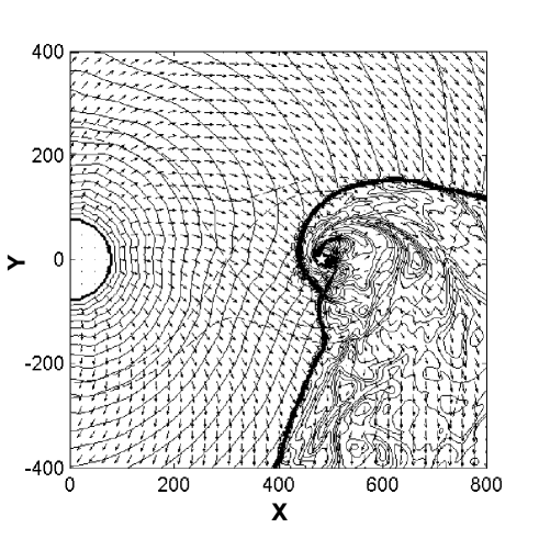
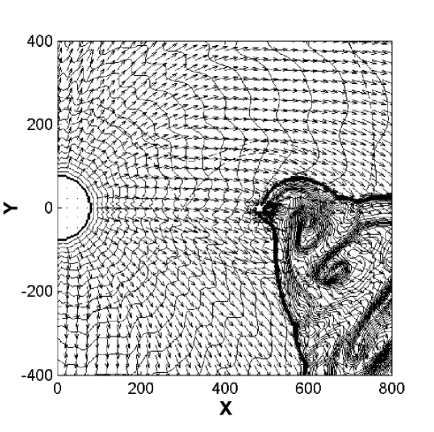
Figure 1: Top panel: Density field and velocity vectors for the stationary case $V=25$ km/s. The isolines of the density logarithm in the range of $10^{-5}$ to 1 (in the units of density at donor’s surface) are shown. The distances are given in solar radii. Dashed lines show equipotential contours of the standard Roche potential. Donor’s surface is shown by the half circle with the center in (0,0) point and the radius $R_{1}$. The star symbol marks accretor. Bottom panel: The same as in the upper panel for the case $V=75$ km/s. Density contours in the bottom panel correspond to density values in the range of 0.04 to 0.55 (in the units of density at the donor’s surface).

The observed values of the wind velocity in symbiotic stars are not far from the value $V=35$ km/s that divides two principally different cases with different accretion regimes. So if at some moment the wind’s velocity increases and exceeds 35 km/s the the disk will be destroyed and the accretion regime will change. It should be mentioned that the value $V=35$ km/s dividing different accretion regimes is also close to the orbital velocity (32 km/s). This fact is in accordance with [16].

In order to consider the process of transition between these two regimes after the wind velocity increase we took the stationary solution for the case $V=25$ km/s, increased the velocity up to $V_{1}$ and continued calculations. Different cases with $V_{1}$ values in the interval 35 km/s $\leq V_{1}\leq 75$ km/s were considered.

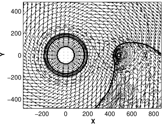
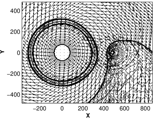
Figure 2: Density field and velocity vectors for the case after wind velocity change from $V=25$ km/s to $V_{1}=40$ km/s. Isolines of the density logarithm in the range of $10^{-5}$ to 1 (in the units of density at donor’s surface) are shown. Distances are given in solar radii. Dashed lines show the equipotential contours of the standard Roche potential. The star symbol marks accretor. Top panel: the moment $0.034P_{orb}$ after the wind velocity change. Bottom panel: the moment $0.073P_{orb}$ after the wind velocity change.

In Figure 2 the morphology of the gas flow – density field and velocity vectors (shown by arrows) – for the case of the wind velocity change from $V=25$ km/s to $V_{1}=40$ km/s is presented. Donor’s surface is shown by the circle with the center in (0,0) point and the radius $R_{1}$. Dashed lines mark the standard Roche equipotential contours. The star symbol marks accretor. Distances are given in the units of the solar radius. Two moments are presented: the first one is for $0.015P_{orb}$ (top panel) and the second one is for $0.05P_{orb}$ (bottom panel) after the wind velocity change. We can see that after the wind velocity change two shocks (seen as condensations of density isolines) propagating from the donor’s surface are formed. Being very close to each other at the first moments they begin to diverge gradually with time. Let us try to explain this phenomenon. Changing of the velocity regime on the surface of mass-losing star results in the collision of two codirectional flows: the ‘new’ one (moving with the radial velocity 40 km/s) and the ‘old’ one (25 km/s). This collision can be described in terms of the Riemann problem. Introducing a new coordinate system moving with the velocity of 32.5 km/s in the radial direction it can be reduced to the frontal collision of two flows with velocities $\pm$7.5 km/s. The solution of this Riemann problem is two diverging shocks moving with velocities (see, e.g., [25])

$$D_{1,2}=\pm\left(\frac{\gamma+1}{4}U+\sqrt{\left(\frac{\gamma+1}{4}U\right)^{2}+c_{s}^{2}}-U\right)\,.$$

Substituting $\gamma=\hbox{$\,{}^{5}\!/_{3}$}$, $U=7.5$ km/s, $c_{s}=5$ km/s we obtain $D_{1,2}=\pm 4.5$ km/s. Coming back to the original coordinate system we obtain two successive shocks with velocities $D_{1}=37$ km/s, $D_{2}=28$ km/s. Note that these values correspond to the first moments of time after the switching of the velocity regime and later will be changed under the action of forces and variation of $c_{s}$.

Let us also estimate the strength of these shocks via the relative pressure jump $\displaystyle\frac{\Delta p}{p_{0}}$, where $\Delta p=p_{1}-p_{0}$, and $p_{0}$, $p_{1}$ are the values of pressure before and after the shocks. Using formulae [25]:

$$\left(\frac{\Delta p}{p_{0}}\right)_{1}=\frac{2\gamma}{\gamma+1}\left(\frac{(D_{1}-V)^{2}}{c_{s}^{2}}-1\right)\,,$$

$$\left(\frac{\Delta p}{p_{0}}\right)_{2}=\frac{2\gamma}{\gamma+1}\left(\frac{(D_{2}-V_{1})^{2}}{c_{s}^{2}}-1\right)\,,$$

and substituting $\gamma=\hbox{$\,{}^{5}\!/_{3}$}$, $c_{s}=5$ km/s, $V=25$ km/s, $V_{1}=40$ km/s, $D_{1}=37$ km/s, $D_{2}=28$ km/s we obtain $\displaystyle\left(\frac{\Delta p}{p_{0}}\right)_{1}=\displaystyle\left(\frac{\Delta p}{p_{0}}\right)_{2}=6$ (the equal strength of two shocks is obvious due to the symmetry of the problem in an appropriate coordinate system).

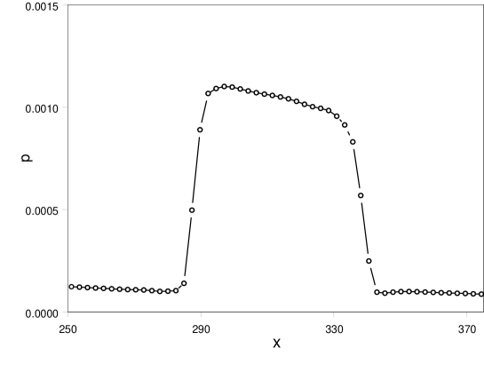
Figure 3: The pressure profile along the $x$ axis in the area near the double shock wave for the moment $0.073P_{orb}$ after the wind velocity change (shown in bottom panel of Fig. 2). Axes in the figure: $x$-axis – distance – in solar radii, $y$-axis – pressure – in relative units.

Figure 3 illustrates the pressure change in the area near the bow shocks. Here we can see that in the area between the two shocks the jump in pressure is in accordance with the above estimates.

When the first of shocks reaches the bow shock located in front of the accretor (after $0.092P_{orb}$ in the case of $V_{1}=40$ km/s) the process of the flow rearrangement near the accretor starts. The coming shocks begin to interact with the matter of the disk and crush it forcing the most part of the matter composing the disk to fall on the accretor’s surface.

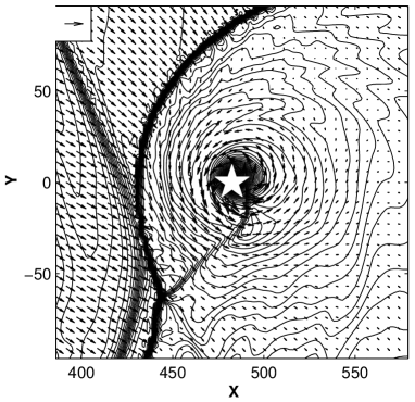
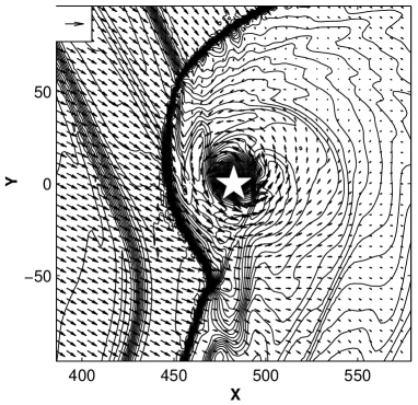
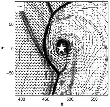
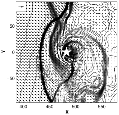
Figure 4: Density field and velocity vectors in the area near the accretor for solution with wind velocity change from $V=25$ km/s to $V_{1}=40$ km/s. The arrow in the left upper corner corresponds to the velocity of 100 km/s. All other designations are the same as in Fig. 1. Four moments are presented: left top panel – $0.092P_{orb}$; right top – $0.110P_{orb}$; left bottom – $0.115P_{orb}$; right bottom – $0.137P_{orb}$ after the wind velocity change.

The set of panels in Figure 4 presents the morphology of the gas flow in the vicinity of the accretor for different moments at early stages of the flow rearrangement. Here the area $[0.8A\ldots 1.2A]\times[-0.2A\ldots 0.2A]$ (or $80\times 80$ grid cells) is presented. After the time of about $0.09P_{orb}$ ($\sim$70 days) after the wind velocity change the first of the two shocks formed reaches the vicinity of the accretor, namely the bow shock in front of it (Fig. 4 – left top panel). The first wave makes the bow shock to come closer to the accretor (see Fig. 4 – right top panel) but the disk still exists. Then ( $\sim 14$ days later) the second wave comes (see Fig. 4 – left bottom panel) and destroys the disk (see Fig. 4 – right bottom panel).

The accretion rate during the flow rearrangement undergoes significant changes. The accretion rate behaviour during the process of the flow rearrangement is presented in Figure 5 for different values of the final wind velocity.

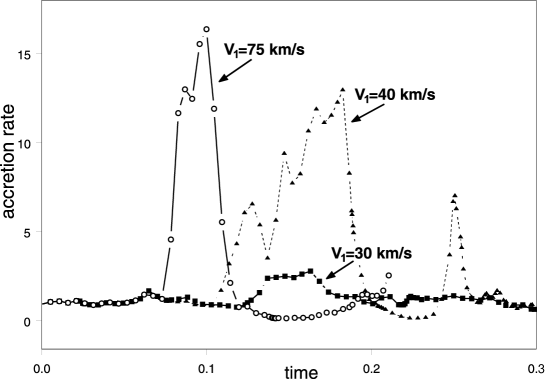
Figure 5: The accretion rate change with time for the cases of wind velocity change from $V=25$ to $V_{1}=$30, 40 and 75 km/s. Time is given in units of the orbital period ($P_{orb}$=758 days), the accretion rate is in percents of the matter that leaves donor’s surface.

We can see that when the final wind velocity $V_{1}$ equals 30 km/s there is no significant increase of the accretion rate while some small variations exist. These variations are probably due to disturbances of the accretion disk by the shock waves formed after the velocity increasing that are not strong enough to crush it. The situation is principally different for other cases – here the jump in the accretion rate takes place. For example, when the final wind velocity is equal to 40 km/s the accretion rate jumps in more than 14 times and in case of 75 km/s – in more than 16 times. This abrupt increase of the accretion rate is caused by the destruction of the accretion disk.

It should be mentioned that the study of the transition period is limited in the framework of this model. After the accretion rate jump the accepted boundary conditions on the accretor change and the model used doesn’t describe the real physical situation any more. Correspondingly, the presented results of calculations of the flow rearrangement period are correct only at first stages of the process.

According to the estimates based on observations [4] in the case of Z And the donor’s wind velocity is $25-40$ km/s when the system is at quiescence. These values of the wind velocity are close to the critical value 35 km/s dividing different accretion regimes. If we suppose the presence of a minor variations of the wind velocity caused, e.g., by the typical giant’s activity [3] the wind velocity can, at some moment, become greater than the critical value. As the consequence the change of the flow structure and of the accretion regime will occur followed by the abrupt jump of the accretion rate in the transition period.

4 Conclusions

The 2D numerical investigation of the gas flow structure in the interacting binary systems with the mass exchange via stellar wind (and namely for their subclass – symbiotic systems) has been carried out using the Roe-Oscher scheme. The modelling has been carried out for different values of the wind velocity. The effect of the velocity change on the system’s behavior was of special interest.

It is shown that after the wind velocity increase the collision of two codirectional flows results in the formation of two shock waves that begin to propagate from the donor’s surface. These shocks can lead to the significant changes in the flow structure near the accreting component and namely to the accretion regime change.

These results were used as the ground for the new mechanism providing the change of the accretion rate and explaining the nature of outbursts in symbiotic stars. The point of this mechanism is in the abrupt change of the flow structure near the accreting component as a result of minor fluctuations of the wind from the mass-losing component. These changes come out in the accretion regime change, namely, in transition from the disk accretion to the accretion from the flow when the wind velocity increases. The process of the flow rearrangement in such cases is followed by the jump in the accretion rate.

Results of modelling of the flow structure in the classical representative of the studied type of binary systems Z And show that in the quiescent state characterized by the wind velocity from 25 to 40 km/s the steady accretion disk forms in the system. In the given regime the accretion efficiency is $\sim$1% of the donor’s mass loss. If the wind velocity increases and becomes greater than 35 km/s the disk disappears and the cone shock wave forms. In stationary solutions for high-velocity regimes ($35-75$ km/s) the accretion rate is slightly higher and equals $\sim$2% of the donor’s mass loss. But during the flow rearrangement when the wind with increased velocity reaches disk and crushes it the accretion rate increases in dozens times!

The analysis of the observations of symbiotic stars during the active stages shows that the most part of the registered manifestations can be explained in terms of the drop-off of the optically thick shell by the accretor [4]. The suggested mechanism provides the accretion rate jump and corresponding increase of the energy release rate large enough to provide the drop-off of the part of the gas from the accretor. Therefore it leads to the appearance of the flow features that can explain the observations.

5 Acknowledgements

This work was partly supported by the Russian Foundation for Basic Research (projects  02-02-16088, 02-02-17642, 00-01-00392), RF President grant 00-15-967221, Federal Programs ”Mathematical Modelling” and ”Astronomy” as well as by INTAS (grant  00-491).

References

1. A. A. Boyarchuk, D. V. Bisikalo, O. A. Kuznetsov and V. M. Chechetkin, Mass Transfer in Close Binary Stars, Taylor&Francis (2002).

2. A. A. Boyarchuk, in Variable Stars and Galaxies, Ed. by B. Warner (ASP Conference Series, 1992), 30, pp. 325–338.

3. J. Mikołajewska and S. J. Kenyon, Monthly Notices Roy. Astron. Soc. 256, 177 (1992).

4. T. Fernandez-Castro, R. Gonzales-Riestra, A. Cassatella, A. R. Taylor and E. R. Seaquist, Astrophys. J. 442, 366 (1995).

5. A. V. Tutukov and L. R. Yungelson, Astrofiz. 12, 521 (1976).

6. B. Paczyński and A. Żytkow, Astrophys. J. 222, 604 (1978).

7. B. Paczyński and B. Rudak, Astron. & Astrophys. 82, 349 (1980).

8. E. M. Sion, M. J. Acierno, and S. Tomczyk, Astrophys. J. 230, 832 (1979).

9. I. Iben, Jr., Astrophys. J., 259, 244 (1982).

10. M. Y. Fujimoto, Astrophys. J. 257, 767 (1982).

11. I. Iben, Jr. and A. V. Tutukov, Astrophys. J. 342, 430 (1989).

12. M. Friedjung, in Cataclysmic Variables and Related Objects, Ed. by M. Hack and C. La Douse (US Gov. Printing Office, Washington, 1993), pp. 647–655.

13. S. J. Kenyon and J. S. Gallagher, Astron. J. 88, 666 (1983).

14. G. S. Bisnovatyi-Kogan, Ya. M. Kazhdan, A. A. Klypin, A. E. Lutskii and N. I. Shakura, Astron. Zh. 56, 359 (1979) [Sov. Astron. 23, 201 (1979)].

15. D. V. Bisikalo, A. A. Boyarchuk, O. A. Kuznetsov and V. M. Chechetkin, Astron. Zh. 71, 560 (1994) [Astron. Reports 38, 494 (1994)].

16. D. V. Bisikalo, A. A. Boyarchuk, O. A. Kuznetsov and V. M. Chechetkin, Astron. Zh. 73, 727 (1996) [Astron. Reports 40, 662 (1996)].

17. E. Kilpio, Odessa Astron. Publ. 14, 41 (2001).

18. T. Theuns and A. Jorissen, Monthly Not. Royal Astron. Soc. 265, 946 (1993).

19. T. Theuns, H. M. J. Boffin, and A. Jorissen, Monthly Not. Royal Astron. Soc. 280, 1264 (1996).

20. K. R. Bell and D. N. Lin, Astrophys. J. 427, 987 (1994).

21. T. Fernandez-Castro, A. Cassatella, A. Gimenez and R. Viotti, Astrophys. J. 324, 1016 (1988).

22. P. L. Roe, Ann. Rev. Fluid Mech. 18, 37 (1986).

23. S. Chakravarthy and S. Osher, AIAA Pap N 85–0363 (1985).

24. D. V. Bisikalo, A. A. Boyarchuk, E. Yu. Kilpio and O. A. Kuznetsov Astron. Zh. 79,(2002) (in press)

25. A. A. Samarskii and Yu. P. Popov, Finite-Difference Methods of Solution of Gas Dynamics, Moscow, Nauka Academic Press (in Russian) (1980).