X-ray and weak lensing measurements of the mass profile of MS1008.1$-$1224: Chandra and VLT data

We analyse the Chandra dataset of the galaxy cluster MS1008.1$-$1224 to recover an estimate of the gravitating mass as function of the radius and compare these results with the weak lensing reconstruction of the mass distribution obtained from deep FORS1-VLT multicolor imaging. Even though the X-ray morphology is disturbed with a significant excess in the northern direction suggesting that the cluster is not in a relaxed state, we are able to match the two mass profiles both in absolute value and in shape within $1\sigma$ uncertainty and up to 1100 $h_{50}^{-1}$ kpc. The recovered X-ray mass estimate does not change by using either the azimuthally averaged gas density and temperature profiles or the results obtained in the northern sector alone where the signal-to-noise ratio is higher.

1 Introduction

As the largest virialized objects in the Universe, galaxy clusters are a powerful cosmological tool once their mass distribution is univocally determined. In the recent past, there have been several claims that cluster masses obtained from X-ray analyses of the intracluster plasma, taken to be in hydrostatic equilibrium with the gravitational potential well, are significantly smaller (up to a factor of two; but see Wu et al. 1998; Allen 1998; Böhringer et al. 1998; Allen et al. 2001) than the ones derived from gravitational lensing (see Mellier 1999 for a review).

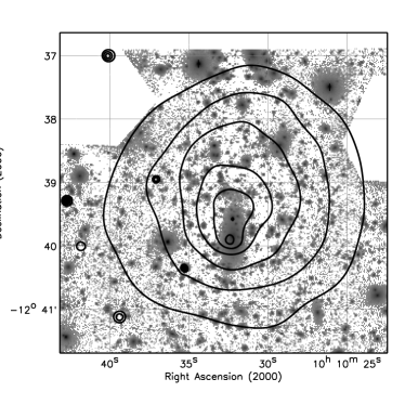
Figure 1: An adaptive smoothed exposure-corrected image in the Chandra [0.5–2] keV band is overplotted to the R-band image (the white areas in the upper end show masked regions). The contours are spaced with steps of $\log 2$ from the minimum of $2.1\times 10^{-9}\mbox{ photon sec}^{-1}\mbox{ cm}^{-2}\mbox{ arcsec}^{-2}$.

In this paper we report on the mass distribution of the cluster MS1008.1$-$1224 by combining the results from weak lensing analysis of deep FORS1-VLT images with those obtained from a spatially-resolved spectroscopic X-ray analysis of a Chandra observation. MS1008.1$-$1224 is a rich galaxy cluster at redshift 0.302 that has been part of the Einstein Medium Sensitivity Survey sample (Gioia & Luppino 1994) and of the CNOC survey (Carlberg et al. 1996). Lombardi et al. (2000) presented a detailed weak lensing analysis of the FORS1-VLT data. Figure 1 shows the X-ray isophotes overplotted to the optical V-band image. In the following we adopt the conversion $1\mbox{ arcmin}=376\mbox{ kpc}$ ($z=0.302$, $H_{0}=50\,h_{50}\mbox{ km s}^{-1}\mbox{ Mpc}^{-1}$, $\Omega_{\rm m}=1-\Omega_{\Lambda}=0.3$) and quote all the errors at $1\sigma$ ($68.3\%$ confidence level).

2 X-ray mass

We retrieved the primary and secondary data products from the Chandra archive. The exposure of MS1008.1$-$1224 was done on June 11, 2000 using the ACIS-I configuration. We reprocessed the level=1 events file in the Very Faint Mode and, then, with the CtiCorrector software (v. 1.38; Townsley et al. 2000). The light curve was checked for high background flares that were not detected. About $44.0\mbox{ ksec}$ (out of $44.2\mbox{ ksec}$, the nominal exposure time) were used and a total number of counts of about $20\,000$ were collected from the region of interest in the 0.5–7 keV band. We used CIAO (v. 2.2; Elvis et al. 2002, in prep.) and our own IDL routines to prepare the data to the imaging and spectral studies. The X-ray center was fixed to the peak of the projected mass from weak lensing analysis (Lombardi et al. 2000) at (RA, Dec; 2000)${}=(10^{\mathrm{h}}10^{\mathrm{m}}32\aas@@fstack{s}68,-12^{\circ}39^{\prime}58.8")$. Note that the maximum value in a $5\arcsec$-smoothed image of the cluster X-ray emission is at (RA, Dec)${}=(10^{\mathrm{h}}10^{\mathrm{m}}32\aas@@fstack{s}44,-12^{\circ}39^{\prime}55.6")$, i.e. less than 5 arcsec apart from the adopted center. With respect to the adopted center, a clear asymmetry in the surface brightness distribution is however detected, suggesting an excess in emission in the northern region (see Fig. 2).

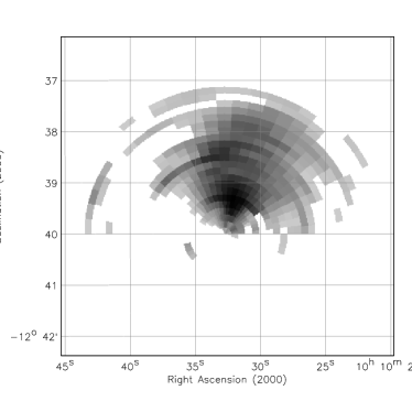
Figure 2: Residuals above $2$ in the X-ray brightness distribution. Given two regions, $A$ and $B$, of (length, width)${}=(8$ arcsec$,20^{\circ})$ located symmetrically with respect to the center and with $C_{A}$ and $C_{B}$ observed counts respectively, the residuals are estimated as $\sigma=(C_{A}-C_{B})/\sqrt{C_{A}+C_{B}}$. An azimuthal scan with step of $20^{\circ}/3$ was done to smooth the map. The most significant excess is along $63^{\circ}\pm 10^{\circ}$ (anticlockwise, from X-axis) with a power of 0.87 estimated as the fraction of regions with higher excess along a fixed direction.

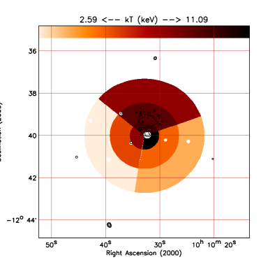
Figure 3: Map of the distribution of the gas temperature according to the structures present in the X-ray surface brightness (see Fig. 2 and Sect.2.1). The code color represents also the variation in the range $(-3.1,+2.1)\sigma$ with respect to the global value of $7.2\mbox{ keV}$.

2.1 X-ray analysis

We detected extended emission at $2\sigma$ confidence level up to 4.1 arcmin ($1.55\mbox{ Mpc}$) and we were able to extract a total of four spectra with about $2\,000$ source counts each to put reasonable constraints on the plasma temperature profile up to $1140\mbox{ kpc}$. The contribution from the source to the total count rate decreases from more $95\%$ in the innermost spectrum to about $30\%$ in the outermost one. We also evaluated the distribution of the plasma temperature values in sectors according to the asymmetrical surface brightness shown in Fig. 2. These best-fit values for a two-dimensional map and for an azimuthally averaged profile are represented in Figs. 3 and 4.

We obtained the Redistribution Matrix Files (RMFs) and Auxiliary Response Files (ARFs) by using the CIAO routines mkrmf and mkarf with the QEU files included in the CtiCorrector package. An emission from an optically-thin plasma (Mekal – Kaastra 1992, Liedhal et al. 1995, in XSPEC v. 11.1.0 – Arnaud 1996) with the metal abundance fixed to 0.3 times the solar value (Anders & Grevesse 1989) and absorbed from the interstellar medium parametrized using the Tübingen-Boulder model (tbabs in XSPEC; Wilms, Allen & McCray 2000) was adopted to reproduce the observed spectra. A galactic column density fixed to $7.0\times 10^{20}\mbox{ cm}^{-2}$ (from radio HI maps in Dickey & Lockman 1990) was assumed. A local background was adopted also considering the relatively high column density of this field with respect to the blank field available for the same CCD and the proper observational period. The overall spectral fit of the counts collected within $1100\mbox{ kpc}$ from the adopted center provides an emission weighted temperature of $7.2^{+1.0}_{-0.8}\mbox{ keV}$ and a bolometric luminosity of $1.6\times 10^{45}\mbox{ erg s}^{-1}$ ($0.9\times 10^{45}$ in the $2$–$10\mbox{ keV}$ band).

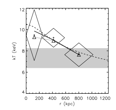
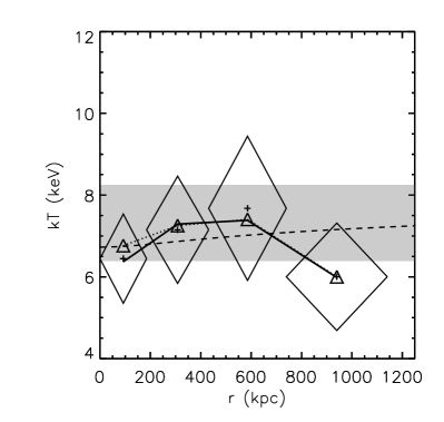
Figure 4: Projected (triangles, dotted line) and deprojected (diamonds) gas temperature profiles. The solid line shows the best-fit applying the hydrostatic equation in combination with the deprojected electron density as discussed in Sect. 2.2. The dashed line indicates the best-fit from a polytropic model. Results for the North excess (left) and for azimuthally averaged profile (right) are shown with overplotted the $1\sigma$ range of emission-weighted temperature up to $110\mbox{ kpc}$.

2.2 X-ray mass profile

In accordance with the weak lensing analysis described in the following section, we assume a spherical geometry for both the dark matter halo and the X-ray emitting plasma (note that negligible effects, when compared with our statistical uncertainties, can be introduced on the mass estimate due to the aspherical X-ray emission, see, e.g., Piffaretti et al. 2002). The values of gas density and temperature in volume shells are recovered from the projected spectral results as described in Ettori et al. (2002). To measure the total gravitating mass $M_{\mathrm{tot}}$, we then constrained the parameters of an assumed mass model by fitting the deprojected gas temperature (shown in Fig. 4) with the temperature profile obtained by inversion of the equation of the hydrostatic equilibrium between the dark matter potential and the intracluster plasma,

$$-G\mu m_{\rm p}\frac{n_{\rm e}M_{\rm tot,model}(<r)}{r^{2}}=\frac{d\left(n_{\rm e}\ kT\right)}{dr}\;.$$ (1)

In this equation, $\mu=0.6$ is the mean molecular weight in a.m.u., $G$ is the gravitational constant, $m_{\rm p}$ is the proton mass, and $n_{\rm e}$ is the deprojected electron density. We considered both the King approximation to the isothermal sphere (King 1962) and a Navarro, Frenk & White (1997) dark matter density profile as mass models (see details in Ettori et al. 2002). By fitting the temperature profile in Fig. 4, we measured the best fit parameters $(r_{\rm s},c)=(646\pm 390,4.2\pm 0.9)$ for a King and $(1122\pm 287,2.3\pm 0.8)$ for a NFW mass model.

Using a $\beta$-model (Cavaliere & Fusco-Femiano 1976) and the ROSAT HRI surface brightness profile detected up to about $765\mbox{ kpc}$ at the $2\sigma$ level, Lewis et al. (1999) measured $M_{\rm tot}=(3.8\pm 0.6)\times 10^{14}M_{\odot}$, assuming an isothermal gas temperature of $7.3\mbox{ keV}$. If we apply a $\beta$-model to our surface brightness profile and a polytropic function to the gas temperature profile, we obtain $r_{\mathrm{c}}=0.264^{+0.025}_{-0.022}\mbox{ Mpc}$, $\beta=0.618^{+0.025}_{-0.031}$ and $\gamma=0.96^{+0.15}_{-0.16}$. The derived mass estimate is lower by $10$–$20\%$ (by $12\%$ at $765\mbox{ kpc}$) than the one in Lewis et al. (1999). The best-fit mass models give $M_{\mathrm{tot,King}}=(4.5\pm 1.2)\times 10^{14}M_{\odot}$ and $M_{\mathrm{tot,NFW}}=(3.2\pm 0.5)\times 10^{14}M_{\odot}$, in agreement with the results obtained from each independent sector of the temperature map in Fig. 3 [e.g., the region to North, which has a higher signal-to-noise ratio due to the excess in brightness, gives $M_{\rm tot,King}=(4.5\pm 0.8)\times 10^{14}M_{\odot}$ and $M_{\rm tot,NFW}=(4.1\pm 0.6)\times 10^{14}M_{\odot}$].

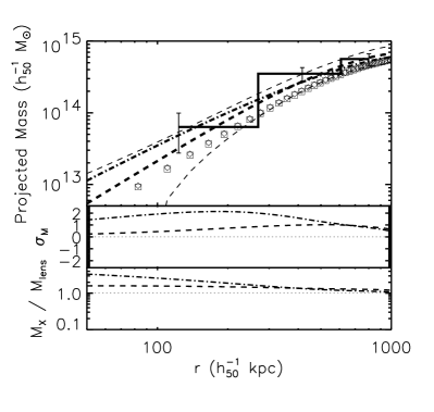
Figure 5: Projected X-ray total gravitating mass profile (with relative error) obtained directly from the electron density and temperature profiles is shown as histogram. Cumulative projected mass profiles from X-ray best-fit mass model (King: dashed line; NFW: dot-dashed line) and weak lensing analysis (squares/B band, diamonds/V band) are overplotted. The deviations in $\sigma$ and in the value of the ratio between X-ray best-fit mass model and weak lensing projected masses are plotted in the panels at the bottom.

3 Weak lensing mass

A weak lensing analysis of MS1008.1$-$1224 using VLT-FORS1 images was carried out by Lombardi et al. (2000) and is summarized below. A parallel weak lensing analysis carried out by Athreya et al. (2002), leads to a mass estimates in agreement with the one presented here.

3.1 Weak lensing analysis

The weak lensing analysis was performed independently on the four (B, V, R, and I) FORS-1 optical images using the IMCAT package (Kaiser et al. 1995; see also Kaiser & Squires 1993). After generating source catalogs, we separated stars from galaxies; the measured sizes and ellipticities of stars were used to correct the galaxy ellipticities for the PSF (see Kaiser et al. 1995; Luppino and Kaiser 1997). The observed galaxies were classified as foreground, background, and cluster members using, when available, the redshift from the CNOC survey (Yee et al. 1998), or the observed colors otherwise. Finally, we used the fiducial background galaxies to obtain the shear field of the cluster and, from this, the projected mass distribution (see Lombardi & Bertin 1999).

Our study differs on a few points with respect to similar weak lensing analyses:

• We decided to use a robust, median estimator to obtain the local shear map from the galaxy ellipticities instead of the more common simple average. In particular, we estimated the local shear on each point of the map by taking a (weighted) median on the observed ellipticities of angularly close background galaxies (see Sect. 4.4 of Lombardi et al. 2000). This way we make sure that a few galaxies with poorly determined ellipticities do not significantly affect the shear estimation.

• We estimated the background sources redshift distribution by resampling the catalog of photometric redshifts of Fernández-Soto et al. (1999) in the Hubble Deep Field.

• We took advantage of the multi-band observations by performing the weak lensing analyses on each band separately.

3.2 Weak lensing mass profile

The reconstructed two-dimensional mass distribution appears to be centered on the cD galaxy and shows elliptical profiles oriented in direction North-South. No substructure on scales larger than $30^{\prime\prime}$ was detected. In order to remove the mass-sheet degeneracy (see, e.g., Kaiser & Squires 1993), we fitted the mass profiles with non-singular isothermal sphere models; from this we obtain, for example, $M(r<1\,h_{50}^{-1}\mbox{ Mpc})=5.3\times 10^{14}\,h_{50}^{-1}\mbox{M}_{\odot}$. We note that, because of the smoothing operated in the two-dimensional mass maps, the weak lensing mass profile for $r<1^{\prime}$ is bound to be underestimate. On the other hand, at large radii (say, $r>3^{\prime}$), an error on the removal of the mass-sheet degeneracy can in principle lead to an unreliable “total” weak lensing mass estimate. Note that the four profiles (from B, V, R and I optical images) agree very well to each other, which strongly support the results of our analysis.

4 Conclusions

The differential X-ray best-fit mass model has been weighted by the relative portion of the shell observed in each ring and, then, cumulated up to the radius of 1020 kpc (the outer radius of our spatially resolved spectroscopy). In Fig. 5, we plot and compare the projected mass profiles of the galaxy cluster MS1008.1$-$1224 obtained from both the spatially resolved spectral analysis of the Chandra observation and the weak lensing analysis of FORS1-VLT multicolor imaging. The two independently reconstructed mass profiles agree very well within $1\sigma$ uncertainty both in absolute values and in the overall shape of the profile. Note that the mass center is fixed to the peak of the lensing map density that is consistent with the X-ray peak as discussed in Sect. 2. This result does not change when we consider the different density and temperature profiles observed in the northern region where a significant surface brightness excess is located and a higher signal-to-noise ratio is available, arguing for the robustness of the X-ray mass estimates once gas density and temperature distributions can be properly mapped.

References

- (1) Allen S.W., 1998, MNRAS, 296, 392
- (2) Allen S.W., Ettori S., Fabian A.C., 2001, MNRAS, 324, 877
- (3) Anders E., Grevesse N., 1989, Geochimica et Cosmochimica Acta, 53, 197
- (4) Arnaud K.A., 1996, ”Astronomical Data Analysis Software and Systems V”, eds. Jacoby G. and Barnes J., ASP Conf. Series vol. 101, 17
- (5) Athreya R.M., Mellier Y., van Waerbeke L., Pelló R., Fort B., Dantel-Fort M., 2002, A&A, 384, 743
- (6) Böhringer H. Tanaka Y., Mushotzky R.F., Ikebe Y., Hattori M., 1998, A&A, 334, 789
- (7) Carlberg R.G., Yee H.K.C., Ellingson E., Abraham R., Gravel P., Morris S., Pritchet C.J., 1996, ApJ, 462, 32
- (8) Cavaliere A., Fusco-Femiano R., 1976, A&A, 49, 137
- (9) Dickey J.M., Lockman, F.J., 1990, ARA&A, 28, 215
- (10) Ettori S., De Grandi S., Molendi S., 2002, A&A, 391, 841
- (11) Fernandez-Soto A., Lanzetta K.M., Yahil A., 1999, ApJ 513, 34
- (12) Gioia I.M., Luppino G.A., 1994, ApJS, 94, 583
- (13) Kaastra J.S., 1992, An X-Ray Spectral Code for Optically Thin Plasmas (Internal SRON-Leiden Report, updated version 2.0)
- (14) Kaiser N., Squires G., 1993, ApJ 404, 441
- (15) Kaiser N., Squires G., Broadhurst T., 1995, ApJ 449, 460
- (16) King I.R., 1962, AJ, 67, 471
- (17) Lewis A.D., Ellingson E., Morris S.L., Carlberg R.G., 1999, ApJ, 517, 587
- (18) Liedahl D.A., Osterheld A.L., Goldstein W.H., 1995, ApJ, 438, L115
- (19) Lombardi M., Bertin G., 1999, A&A 348, 38
- (20) Lombardi M., Rosati P., Nonino M., Girardi M., Borgani S., Squires G., 2000, A&A, 363, 401
- (21) Luppino G.A., Kaiser N., 1997, ApJ 475, 20
- (22) Mellier Y., 1999, ARAA, 37, 127
- (23) Navarro J.F., Frenk C.S., White S.D.M., 1997, ApJ, 490, 493
- (24) Piffaretti R., Jetzer Ph., Schindler S., 2002, A&A, in press (astro-ph/0211383)
- (25) Townsley L.K., Broos P.S., Garmire G.P., Nousek J.A., 2000, ApJ, 534, L139
- (26) Yee H.K.C., Ellingson E., Morris S.L., Abraham R.G., Carlberg R.G., 1998, ApJS 116, 211
- (27) Wilms J., Allen A., McCray R., 2000, ApJ, 542, 914
- (28) Wu X.P., Chiueh T., Fang L.Z., Xue Y.J., 1998, MNRAS, 301, 861