Compressible MHD Turbulence: Mode Coupling, Anisotropies and Scalings

Abstract

Compressible turbulence, especially the magnetized version of it, traditionally has a bad reputation with researchers. However, recent progress in theoretical understanding of incompressible MHD as well as that in computational capabilities enabled researchers to obtain scaling relations for compressible MHD turbulence. We discuss scalings of Alfven, fast, and slow modes in both magnetically dominated (low $\beta$) and gas pressure dominated (high $\beta$) plasmas. We also show that the new regime of MHD turbulence below viscous cutoff reported earlier for incompressible flows persists for compressible turbulence. Our recent results show that this leads to density fluctuations. New understanding of MHD turbulence is likely to influence many key astrophysical problems.

0.1 ISM and MHD Turbulence

The interstellar medium (ISM) in spiral galaxies is crucial for determining the galactic evolution and the history of star formation. The ISM is turbulent on scales ranging from AUs to kpc (Armstrong et al 1995; Stanimirovic & Lazarian 2001; Deshpande et al 2000), with an embedded magnetic field that influences almost all of its properties. This turbulence holds the key to many astrophysical processes (star formation, the phases, spatial distribution, heating of the ISM, and others).

Present codes can produce simulations that resemble observations (e.g., Vazquez-Semadeni et al 2000, Vazquez-Semadeni 2000). To what extent do these results reflect reality? A meaningful numerical representation of the ISM requires some basic non-dimensional combinations of the physical parameters of the simulation to be similar to those of the real ISM. One such parameter is the “Reynolds number”, $Re$, the ratio of the eddy turnover time of a parcel of gas to the time required for viscous forces to slow it appreciably. A similar parameter, the “magnetic Reynolds number”, $Rm$, is the ratio of the eddy turnover time to magnetic field decay time. The properties of the flows on all scales depend on $Re$ and $Rm$. Flows with $Re<100$ are laminar; chaotic structures develop gradually as $Re$ increases, and those with $Re\sim 10^{3}$ are appreciably less chaotic than those with $Re\sim 10^{7}$. Observed features such as star forming clouds are very chaotic with $Re>10^{8}$ and $Rm>10^{16}$. The currently available 3D simulations for a $512^{3}$ grid can have $Re$ and $Rm$ up to $\sim 6000$ and are limited by their grid sizes. It should be kept in mind that while low-resolution observations show true large-scale features, low-resolution numerics may produce a completely incorrect physical picture.

How feasible is it, then, to strive to understand the complex microphysics of astrophysical MHD turbulence? Substantial progress in this direction is possible by means of “scaling laws”, or analytical relations between non-dimensional combinations of physical quantities that allow a prediction of the motions over a wide range of $Re$. Even with its limited resolution, numerical simulation is a great tool to test scaling laws.

In spite of its complexity, turbulent cascade is remarkably self-similar. The physical variables are proportional to simple powers of the eddy size over a large range of sizes, leading to scaling laws expressing the dependence of certain non-dimensional combinations of physical variables on the eddy size. Robust scaling relations can predict turbulent properties on the whole range of scales, including those that no large-scale numerical simulation can hope to resolve. These scaling laws are extremely important for obtaining insights of processes on the small scales.

By using scaling arguments, Goldreich & Sridhar (1995) made ingenious predictions regarding relative motions parallel and perpendicular to magnetic field B for Alfvenic turbulence. These relations have been confirmed numerically (Cho & Vishniac 2000; Maron & Goldreich 2001; Cho, Lazarian & Vishniac 2002a; see also Cho, Lazarian & Vishniac 2002b, henceforth CLV02 for a review); they are in good agreement with observed and inferred astrophysical spectra (CLV02). A remarkable fact revealed in Cho, Lazarian & Vishniac (2002a) is that fluid motions perpendicular to B are identical to hydrodynamic motions. This provides an essential physical insight and explains why in some respects MHD turbulence and hydrodynamic turbulence are similar, while in other respects they are different.

The Goldreich & Sridhar (1995, henceforth GS95) model considered incompressible MHD, but the real ISM is highly compressible. This motivated further studies of the compressible mode scalings.

Figure 1: Generation of compressible modes from decaying Alfven Turbulence. Generation is marginal. (Left Panel) Time evolution. Initially only Alfven modes exist. As time goes on, compressible modes are spontaneously generated. Initially, $\beta\sim 0.2$ and $B_{0}/\sqrt{4\pi\rho_{0}}=1$. (Middle Panel) Generation of slow modes as a function of $B_{0}^{2}$. (Right Panel) Generation of fast modes as a function of $B_{0}$. From Cho & Lazarian (CL02).

0.2 Effects of Compressibility

Three types of waves exist in compressible magnetized plasma. They are Alfven, slow and fast waves. Turbulence is a highly non-linear phenomenon and it has been thought that it may not be productive to talk about different types of perturbations or modes in compressible media as everything is messed up by strong interactions. Although the statements of this sort dominate the MHD literature one may question how valid they are. If, for instance, one particular type of perturbations cascades to small scales faster than it interacts with the other types, its cascade should proceed on its own. Within the GS95 model the Alfvenic perturbations cascade to small scales over their period, while the other non-linear interactions are longer. Therefore we would expect that the GS95 scaling for Alfven modes should be present in compressible turbulence as well.

Some hints about effects of compressibility can be inferred from Goldreich & Sridhar (1995) seminal paper. A more focused theoretical analysis was done in Lithwick & Goldreich (2001) paper which deals with properties of pressure dominated plasma, i.e. in high $\beta$ regime, where $\beta\equiv P_{gas}/P_{mag}\gg 1$. Incompressible regime formally corresponds to $\beta\rightarrow\infty$ and therefore it is natural to expect that for $\beta\gg 1$ the turbulence picture proposed in GS95 would persist. The only actual difference between subsonic turbulence in high $\beta$ and incompressible regimes is that for finite $\beta$ a new type of motions, fast modes, is present. Those modes for pressure dominated environments are analogous to sound waves which are marginally affected by magnetic field. Therefore it is natural to expect that they will not distort the GS95 picture of MHD cascade. Lithwick & Goldreich (2001) also speculated that for low $\beta$ plasmas the GS95 picture may still be applicable.

A systematic study of the compressibility in low $\beta$ plasmas was done by Cho & Lazarian (2002, henceforth CL02). First of all, we tested the coupling of compressible and incompressible modes. If Alfvenic modes produce a copious amount of compressible modes, the whole picture of independent Alfvenic turbulence fails. However, the calculations (see Fig 1) show that the amount of energy drained into compressible motions is negligible, provided that the external magnetic field is sufficiently strong.

Figure 2: Low $\beta$. Spectra and eddy shapes from driven turbulence with $M_{s}\sim 2.2$, $M_{A}\sim 0.7$, $\beta\sim 0.2$, and $216^{3}$ grid points. (a) Spectra of Alfvén modes follow a Kolmogorov-like power law. (b) Eddy shapes (contours of same second-order structure function, $SF_{2}$) for velocity of Alfvén modes shows anisotropy similar to the GS95 ($r_{\|}\propto r_{\perp}^{2/3}$ or $k_{\|}\propto k_{\perp}^{2/3}$). The structure functions are measured in directions perpendicular or parallel to the local mean magnetic field in real space. We obtain real-space velocity and magnetic fields by inverse Fourier transform of the projected fields. (c) Spectra of slow modes also follow a Kolmogorov-like power law. (d) Slow mode velocity shows anisotropy similar to the GS95. We obtain contours of equal $SF_{2}$ directly in real space without going through the projection method, assuming slow mode velocity is nearly parallel to local mean magnetic field in low $\beta$ plasmas. (e) Spectra of fast modes are compatible with the IK spectrum. (f) The magnetic $SF_{2}$ of fast modes shows isotropy. We obtain real-space magnetic field by inverse Fourier transform of the projected fast magnetic field. Fast mode velocity also shows isotropy. From CL02.

When the decoupling of the modes was proved, it became meaningful to talk about separate cascades. A remarkable feature of the GS95 picture is that turbulent cascade of Alfven waves happens over just one wave period. Therefore the non-linear interactions with other types of waves affect the cascade only marginally and the GS95 scaling is expected to persist in the compressible medium. Moreover, as the Alfven waves are incompressible, their cascade persists even for supersonic turbulence. In low $\beta$ regime the slow modes are sound-type perturbations moving along magnetic fields with velocity $a$ (or, $a\cos\theta$ in the direction of wave vector ${\bf k}$), where $a$ ($=\sqrt{\gamma P_{gas}/\rho}$) is the sound velocity and $\theta$ is the angle between the wavevector and magnetic field. In magnetically dominated environments $a\ll V_{A}$, the gaseous perturbations are essentially static and the magnetic field mixing motions are expected to mix density perturbations as if they were passive scalar. As the passive scalar shows the same scaling as the velocity field of the inducing turbulent motions, the slow waves are expected to demonstrate GS95 scalings. The fast waves in low $\beta$ regime propagate at $V_{A}$ irrespectively of the magnetic field direction. Thus the mixing motions induced by Alfven waves should affect the fast wave cascade only marginally. The latter cascade should be analogous to the acoustic wave cascade and be isotropic.

To separate the fast, Alfven and slow modes of MHD turbulence was the task solved in CL02. Earlier researchers were probably not much motivated to attempt this, as it was generally believed that the different modes are messed up in turbulence anyhow. To separate the modes, let us consider the displacement vector $\xi$. For example, $\xi_{f}({\bf k})$ denotes the direction of displacement for the fast mode with wave vector ${\bf k}$. In CL02, we showed that fast, slow, and Alfven displacement vectors ($\xi_{f}$, $\xi_{s}$, and $\xi_{A}$, respectively) can be written in terms of ${\bf k}_{\|}$ and ${\bf k}_{\perp}$:

$${\bf\xi}_{f}({\bf k})\propto\frac{-1+\alpha+\sqrt{D}}{1+\alpha+\sqrt{D}}k_{\|}\hat{\bf k}_{\|}+k_{\perp}\hat{\bf k}_{\perp},$$ (1)

$${\bf\xi}_{s}({\bf k})\propto k_{\|}\hat{\bf k}_{\|}+\frac{1+\alpha-\sqrt{D}}{-1+\alpha-\sqrt{D}}k_{\perp}\hat{\bf k}_{\perp},$$ (2)

$${\bf\xi}_{A}({\bf k})\propto{\bf k}_{\|}\times{\bf k}_{\perp},$$ (3)

where ${\bf k}_{\|}$ (or ${\bf k}_{\perp}$) is the wave vector parallel (or perpendicular) to the mean field ${\bf B}_{0}$, $\alpha=a^{2}/V_{A}^{2}=\beta\gamma/2$, and $D=(1+\alpha)^{2}-4\alpha\cos^{2}\theta$. After proper normalization, we get a set of unit bases (${\bf\xi}_{f}({\bf k}),{\bf\xi}_{s}({\bf k}),{\bf\xi}_{A}({\bf k})$). These unit vectors are well-defined and mutually perpendicular except on the ${\bf k}_{\|}$ axis. We can get fast, slow, or Alfven component velocity by projecting the Fourier velocity component $\hat{\bf v}({\bf k})$ onto these unit bases. See CL02 and Cho & Lazarian (preprint) for details.

Results of the CL02 study are shown in Fig 2. The calculations confirm the theoretical considerations provided above. Indeed, both the spectra and anisotropies obtained for Alfven and slow modes look remarkably similar to the earlier incompressible runs (see Fig 3 where both the data and analytical fit for the isocontours of equal correlation are shown).

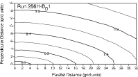
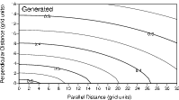
Figure 3: (a) Iso-contours of equal (velocity) correlation from a simulation. The contours represent shape of different size eddies. The smaller contours (or, eddies) are more elongated. (b) Contours generated from analytical formula.From Cho, Lazarian, & Vishniac (2002a).

Our more recent results for high $\beta$ plasma are shown in Fig 4. They confirm theoretical considerations in Lithwick & Goldreich (2001). This means that for the first time we have a theoretical insight and simple scaling relations working for high $\beta$ and low $\beta$ MHD turbulence. What will happen in the regime of moderate $\beta$?

Figure 4: High $\beta$. Spectra and eddy shapes from driven turbulence with $M_{s}\sim 0.5$, $M_{A}\sim 0.7$, $\beta\sim 4$, and $216^{3}$ grid points. See captions in Fig. 2. From Cho & Lazarian (in prep.).

We would speculate that due to its rapid cascade the Alfven waves should preserve GS95 scaling. Moreover, the passive nature of the slow modes in both high and low $\beta$ regimes induce us to think that they would mimic the spectrum of Alfven modes in the $\beta\sim 1$ case as well. The decoupling of the fast waves and their isotropy in this regime are also likely. Thus we may hope that we have a picture of MHD turbulence in general and the difference between the aforementioned modes would stem from the difference in the partition of energy between magnetic and gas energies in the compressional modes as $\beta$ varies. For instance, most energy of the slow modes in low $\beta$ plasma is in gas compression, while in high $\beta$ plasma the slow modes energy is mostly magnetic.

How important is the strength of the regular magnetic field? In our computations the magnetic field was taken to be sufficiently strong. If the magnetic field is weak and strongly entangled by turbulence, the decoupling of modes is difficult. One may wonder to what extend our insight above is applicable. We believe that if the magnetic field energy $B^{2}/8\pi$ is much smaller than energy $\rho V_{l}^{2}/2$ at a scale $l$, the magnetic field would not change the dynamics of eddies at this scale and therefore the turbulence would be hydrodynamic. At smaller scales, however, as the energy of eddies decreases (e.g. as $l^{2/3}$ for the Kolmogorov cascade) the magnetic field becomes dynamically important with the implication that the scaling relations tested for the strong external magnetic field should be applicable.

0.3 Ion-neutral damping: a new regime of turbulence

In hydrodynamic turbulence viscosity sets a minimal scale for motion, with an exponential suppression of motion on smaller scales. Below the viscous cutoff the kinetic energy contained in a wavenumber band is dissipated at that scale, instead of being transferred to smaller scales. This means the end of the hydrodynamic cascade, but in MHD turbulence this is not the end of magnetic structure evolution. For viscosity much larger than resistivity, $\nu\gg\eta$, there will be a broad range of scales where viscosity is important but resistivity is not. On these scales magnetic field structures will be created by the shear from non-damped turbulent motions, which amounts essentially to the shear from the smallest undamped scales. The created magnetic structures would evolve through generating small scale motions. As a result, we expect a power-law tail in the energy distribution, rather than an exponential cutoff. This completely new regime for MHD turbulence was reported in Cho, Lazarian & Vishniac (2002c). Further research showed that there is a smooth connection between this regime and small scale turbulent dynamo in high Prandtl number fluids (see Schekochihin et al. 2002).

In partially ionized gas neutrals produce viscous damping of turbulent motions. In the Cold Neutral Medium (see Draine & Lazarian 1999 for a list of the idealized phases) this produces damping on the scale of a fraction of a parsec. The magnetic diffusion in those circumstances is still negligible and exerts an influence only at the much smaller scales, $\sim 100km$. Therefore, there is a large range of scales where the physics of the turbulent cascade is very different from the GS95 picture.

Cho, Lazarian, & Vishniac (2002c) explored this regime numerically with a grid of $384^{3}$ and a physical viscosity for velocity damping. The kinetic Reynolds number was around 100. The result is presented in Fig. 5a.

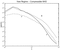
Figure 5: New Regime of MHD turbulence: viscously damped. (a) (Left) Incompressible case. A new inertial range emerges below the viscous cut-off at $k\sim 7$. From Cho, Lazarian, & Vishniac (2002c). (b) (Right) Due to numerical reasons the inertial range is truncated when we use our compressible code. However, the new regime persists and causes density fluctuations. From an upcomming paper.

A theoretical model for this new regime and its consequences for stochastic reconnection (Lazarian & Vishniac 1999) can be found in Lazarian, Vishniac, & Cho (2002). It explains the spectrum $k^{-1}$ as a cascade of magnetic energy to small scales under the influence of shear at the marginally damped scales. Moreover, our work suggests that the magnetic fluctuations protrude to the decoupling scales and cause the renewal of the MHD cascade there. Earlier work, e.g. Lithwick & Goldreich (2001) argued that the turbulent cascade survives ion-neutral damping only when a high degree of ionization is present. In view of the finding a revision of a few earlier theoretical conclusions is necessary. It should be noted that our conclusion about the resumption of turbulence at small scales is consistent with observations (Spangler 1991; 1999) that do not show any change of the observed electron scintillation spectrum at the ambipolar damping scale.

We show our results for the compressible fluid in Fig 5b. The inertial range is much smaller due to numerical reasons, but it is clear that the new regime of MHD turbulence persists. The magnetic fluctuations, however, compress the gas and thus cause fluctuations in density. This is a new (although expected) phenomenon compared to our earlier incompressible calculations. These density fluctuations may have important consequences for the small scale structure of the ISM. We may speculate that they might have some relation to the tiny-scale atomic structures (TSAS). Heiles (1997) introduced the term TSAS for the mysterious H I absorbing structures on scales from thousands to tens of AU, discovered by Dieter, Welch & Romney (1976). Analogs are observed in NaI and CaII (Meyer & Blades 1996; Faison & Goss 2001; Andrews, Meyer, & Lauroesch 2001) and in molecular gas (Marscher, Moore, & Bania 1993).

Our calculations are applicable on scales from the viscous damping scale (determined by equating the energy transfer rate with the viscous damping rate; $\sim 0.1$ pc in the Warm Neutral Medium with $n$ = 0.4 cm^-3, $T$= 6000 K) to the ion-neutral decoupling scale (the scale at which viscous drag on ions becomes comparable to the neutral drag; $\ll 0.1$ pc). Below the viscous scale the fluctuations of magnetic field obey the damped regime shown in Figure 5b and produce density fluctuations. For typical Cold Neutral Medium gas, the scale of neutral-ion decoupling decreases to $\sim 70$ AU, and is less for denser gas. TSAS may be created by strongly nonlinear MHD turbulence!

0.4 Discussion

In this paper we have discussed the new outlook onto compressible MHD turbulence. Contrary to common beliefs the compressible MHD turbulence does not present a complete mess, but demonstrates nice scaling relations for its modes. A peculiar feature is that those relations should be studied locally, i.e. in the frame related to the local magnetic field. However, such a system of reference is natural for many phenomena, e.g. for cosmic ray propagation. Recent application of the scalings obtained for compressible turbulence have shown that fundamental revisions are necessary for the field of high energy astrophysics. For instance, Yan & Lazarian (2002) demonstrated that fast modes dominate cosmic ray scattering even in spite of the fact that they are subjected to collisional and collisionless damping. This entails consequences for models of cosmic ray propagation, acceleration, elemental abundances etc.

Advances in understanding of MHD turbulence have very broad astrophysical implications. The fields affected span from accretion disks and stars to the ISM and the intergalactic medium in clusters. Turbulence is known to hold the key to many astrophysical processes. It was considered too messy by many researchers who consciously or subconsciously tried to avoid dealing with it. Others, more brave types, used Kolmogorov scalings for compressible strongly magnetized gas, although they did understand that those relations could not be true. Recent research in the field provides the scaling relations and insights that will contribute to many areas of research.

- [1] Andrews, S. M., Meyer, D. M., & Lauroesch, J. T. 2001 ApJ, 552, L73
- [2] Armstrong, J. W., Rickett, B. J., & Spangler, S. R. 1995, ApJ, 443, 209
- [3] Cho, J., Lazarian, A. 2002, Phy. Rev. Lett., 88, 245001 (CL02)
- [4] Cho, J., Lazarian, A., & Vishniac, E. 2002a, ApJ, 564, 291
- [5] Cho, J., Lazarian, A., & Vishniac, E. 2002b, in Simulations of magnetohydrodynamic turbulence in astrophysics, eds. T. Passot & E. Falgarone (Springer LNP) (astro-ph/0205286) (CLV02)
- [6] Cho, J., Lazarian, A., & Vishniac, E. 2002c, ApJ, 566, L49
- [7] Cho, J. & Vishniac, E. 2000, ApJ, 539, 273
- [8] Deshpande, A. A., Dwarakanath, K. S., & Goss, W. M. 2000, ApJ, 543, 227
- [9] Dieter,N. H., Welch, W. J., & Romney, J. D. 1976, ApJ, 206, L113
- [10] Draine, B. T. & Lazarian, A. 1999, ApJ, 512, 740
- [11] Faison, M. D. & Goss, W. M. 2001, AJ, 121, 2706
- [12] Goldreich, P. & Sridhar, S. 1995, ApJ, 438, 763
- [13] Heiles, C. 1997, ApJ, 481, 193
- [14] Lazarian, A. & Vishniac, E. T. 1999, ApJ, 517, 700
- [15] Lazarian, A. & Vishniac, E. T., & Cho, J. 2002, ApJ, submitted
- [16] Lithwick, Y. & Goldreich, P. 2001, ApJ, 562, 279
- [17] Maron, J. & Goldreich, P. 2001, ApJ, 554, 1175
- [18] Marscher, A. P., Moore, E. M., & Bania, T. M. 1993, ApJ, 419, L101
- [19] Meyer, D. M. & Blades, J. C. 1996, ApJ, 464, L179
- [20] Schekochihin, A., Maron, J., Cowley, S., & McWilliams, J. 2002, ApJ, 576, 806
- [21] Spangler,S.R. 1991, ApJ, 376, 540
- [22] Spangler,S.R. 1999, ApJ, 522, 879
- [23] Stanimirovic, S. & Lazarian, A. 2001, ApJ, 551, L53
- [24] Vazquez-Semadeni, E. 2000, in Advanced Series in Astrophysics and Cosmology, Vol. 10, eds. V. Gurzadyan & R. Ruffini (World Scientific), p.379
- [25] Vazquez-Semadeni, E., Ostriker, E.C., Passot, T., Gammie, C.F., & Stone, J.M. 2000, in Protostars and Planets IV, eds. V. Mannings et al. (Tucson: University of Arisona Press), p.3
- [26] Yan, H. & Lazarian, H. 2002, Phy. Rev. Lett., in press