Dependence of the Inner DM Profile on the Halo Mass

Abstract

I compare the density profile of dark matter (DM) halos in cold dark matter (CDM) N-body simulations with 1 h^-1 Mpc, 32 h^-1 Mpc, 256 h^-1 Mpc and 1024 h^-1 Mpc box sizes. I compare the profiles when the most massive halos are composed of about $10^{5}$ DM particles. The DM density profiles of the halos in the 1 h^-1 Mpc box at redshift $z\sim 10$ show systematically shallower cores with respect to the corresponding halos in the 32 h^-1 Mpc simulation at $z\sim 3$ that have masses, $M_{dm}$, typical of the Milky Way and are fitted by a NFW profile. The DM density profiles of the halos in the 256 h^-1 Mpc box at $z\sim 0$ are consistent with having steeper cores than the corresponding halos in the 32 h^-1 Mpc simulation, but higher mass resolution simulations are needed to strengthen this result. Combined, these results suggest that the density profile of DM halos is not universal, presenting shallower cores in dwarf galaxies and steeper cores in clusters. More work is needed to validate this finding at $z=0$. Physically the result sustains the hypothesis that the mass function of the accreting satellites determines the inner slope of the DM profile. But the result can also be interpreted as a trend with the dynamical state in the assembly process of halos of different mass. In comoving coordinates, $r$, the profile

$$\rho_{dm}\propto{1\over X^{\alpha}(1+X)^{3-\alpha}}$$

with $X=c_{\Delta}r/r_{\Delta}$ and $\alpha=(9+3n)/(5+n)\approx 1.3+(M_{dm,14}^{1/6}-1)/(M_{dm,14}^{1/6}+1)$, provides a good fit to all the DM halos from dwarf galaxies to clusters at any redshift with the same concentration parameter $c_{\Delta}\sim 7$. Here, $r_{\Delta}(M_{dm})$ is the virial radius, $n$ is the effective spectral index of the initial power spectrum of density perturbations and $M_{dm,14}=M_{dm}/(3\times 10^{14}$ M_⊙). The slope, $\gamma$, of the outer parts of the halo appears to depend on the acceleration of the universe: when the scale parameter is $a=(1+z)^{-1}\lower 2.15277pt\hbox{$\;\buildrel<\over{\sim}\;$}1$, the slope is $\gamma\approx 3$ as in the NFW profile, but $\gamma\approx 4$ at $a>1$ when $\Omega_{\Lambda}\sim 1$ and the universe is inflating. The shape of the DM profiles presents a significant scatter around the mean. It is therefore important to analyse a significant statistical sample of halos in order to determine the mean profile.

I compare the DM profiles in the 1 h^-1 Mpc box with the same simulation including stars, baryons and radiative transfer presented by Ricotti, Gnedin and Shull. Radiative feedback effects produce a larger scatter in the density profile shapes but, on average, do not affect the shape of the DM profiles significantly.

1 Introduction

According to the currently favoured galaxy formation scenarios, galaxies are formed from the gravitational growth of tiny density perturbations imprinted on a uniform universe during inflation. Small mass perturbations grow faster and constitute the building blocks for the assembly of larger galaxies and clusters. In the nonlinear phase of the gravitational collapse the dark matter (DM) particles are shock heated to the virial temperature and settle into a dark halo with mean overdensity about $\Delta=178$ (according to the simple spherical collapse model in a flat $\Omega_{0}=1$ universe). Analysing N-body simulations of hierarchical structure formation Navarro, Frenk & White (1996, 1997) (hereafter, NFW) have proposed that DM halos develop a universal density profile, valid for virialized halos at any redshift and with any mass, from dwarf galaxies to clusters. Further works have shown that an approximatively universal profile develops regardless of the details of the adopted cosmology and initial power spectrum of density perturbations (Huss et al., 1999; Eke et al., 2001). The NFW density profile has a core cusp $\rho\propto r^{-1}$ and in the outer regions the density decreases as $\rho\propto r^{-3}$. The details of the gravitational collapse affect only the relative size of the core with respect to the virial radius (the halo concentration parameter, $c_{\Delta}$) but not the slope of the profile. This result implies that during the virialization process the memory of the mass function and profile shapes of the building blocks that formed the halo is lost.

Recent observations of dwarf galaxies (spheroidal and irregular) and low surface brightness (LSB) galaxies seem to show that a flat core for the DM density profile is more compatible with the measurements of the rotation curves (van den Bosch et al., 2000; de Blok et al., 2001; de Blok & Bosma, 2002; Borriello & Salucci, 2001; Salucci & Burkert, 2000). These observations have renewed interest in the subject and a number of solutions have been proposed to solve this possible discrepancy. The proposed solutions range from feedback effects of the baryons and stars on the DM density profile to modifications of the physical properties (e.g., scattering cross section, temperature) of the DM particles. Some examples of alternatives to CDM are warm dark matter (Bode et al., 2001) and self-interacting DM (Spergel & Steinhardt, 2000). The potential discrepancy between the steep DM cores found in N-body simulations with the observed flat core of dwarf galaxies is perhaps the most serious problem faced in CDM cosmologies today.

High resolution simulations and careful convergence tests have been done or are underway to understand if the discrepancies found by some authors (e.g., Moore et al. (1998, 1999) find steeper core profiles) are due to numerical artifacts. In the core of DM halos the particle crossing time is much shorter than the Hubble time and the integration of trajectories is subject to subtle numerical effects that are difficult to keep under control. Power et al. (2002) estimated that about 1 million particles are needed in order to have convergent results in the inner 1% of the halo virial radius. To have such a high number of particles per halo the use of a special technique is required. This technique consists of simulating with high mass resolution only the particles that will end up in the halo of interest at $z=0$, while having less mass resolution for the particles that end up far away from the halo of interest. This has the drawback that each simulation can resolve only one halo at a time, therefore selection effect biases and a poor statistical sample could affect the reliability of the final result even if the simulation is very accurate and has high resolution. Note that most of the detailed and computationally expensive work on the subject has focused on simulating halos at $z=0$ with typical mass similar to the Milky Way.

The mass function of the building blocks of dwarf galaxies is different in comparison to the one for larger galaxies or clusters. On small scales (or masses) the mass fraction of virialized halos is about constant as a function of the logarithmic DM mass of the halos because the power spectrum has a slope $n\sim-3$. This means that small and large mass satellites contribute equally to the mass of the accreting halo. In massive halos as in the Milky Way or in clusters of galaxies, the contribution from large mass accreting satellites is instead dominant. For this reason it is more crucial to resolve very small mass satellites (i.e., to have high mass resolution) in simulating dwarf galaxies than in simulating massive galaxies or clusters.

In this paper I compare the density profiles of DM halos in four CDM N-body simulations that are identical apart from the box sizes that are 1 h^-1 Mpc, 32 h^-1 Mpc, 256 h^-1 Mpc and 1024 h^-1 Mpc. The simulation method is a two-level particle-particle particle-mesh (P³M) with $256^{3}$ particles and $\Lambda$CDM cosmology. In dimensionless units the only difference between the simulations is the initial power spectrum of density perturbations. I compare the profiles when the most massive halos are composed of about $10^{5}$ DM particles and the clustering in the simulations is similar (see Fig. 2). This is done in order to minimise possible systematic errors in the simulations and to be more confident that any variation in the profile shapes is produced by the different initial power spectrum. The masses of the halos studied in the four simulations, from the small to the large box, are typical of dwarf galaxies, Milky Way mass galaxies, clusters and superclusters of galaxies, respectively.

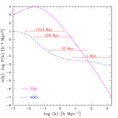
Figure 1: Linear power spectrum of density fluctuations at $z=0$ (solid line) and logarithmic slope, $n(k)$, of the power spectrum (dashed line). The horizontal bars show the range of wave numbers, $k=2\pi/\lambda$, resolved in the $1,32,256$ and $1024$ h^-1 Mpc simulations.

If the cores of small mass halos are dense enough to resist disruption and survive “undigested” when incorporated into a larger object, they should determine the halo structure in the inner regions. Using scaling arguments Subramanian, Cen & Ostriker (2000) have shown that, in a flat universe with an initial power spectrum of density perturbation $P(k)\propto k^{n}$, the core density profile is $\rho_{dm}\propto r^{\alpha}$ with $\alpha=(9+3n)/(5+n)$. The numerical results that they report approximately confirm this expectation. In $\Lambda$CDM cosmologies the logarithmic slope of the initial power spectrum ranges between $-3<n<1$, depending on the mass scale (see Fig. 1). From dwarfs to superclusters the logarithmic slope of the core density profile should range between $0\lower 2.15277pt\hbox{$\;\buildrel<\over{\sim}\;$}\alpha\lower 2.15277pt\hbox{$\;\buildrel<\over{\sim}\;$}2$. As shown in Fig. 1, the power spectrum in the 1 h^-1 Mpc box is a power law with $n\approx-2.7$. According to the aforementioned scaling relationship $\alpha\approx 0.4$. This slope is in agreement with what I find in the 1 h^-1 Mpc box. In the 32 h^-1 Mpc box the power spectrum is not a single power law but the slope is close to $n\approx-2$ and therefore $\alpha\approx 1$ is expected, consistent with the NFW universal profile and with the result found for this simulation. In cluster and supercluster size halos $\alpha$ should be larger than in galaxy size halos ($\alpha\sim 1.5$). Indeed, in the 256 h^-1 Mpc simulation I find slopes of the inner profile $\alpha\sim 1.4$. But this is not a strong result because the number of particles in each halo is barely sufficient to start seeing a deviation with respect to the NFW profile. Moreover, the introduction of the parameter $\alpha$ for the slope of the inner part of the halo profile (which can be easily calculated knowing the mass of the galaxy halo) does not increase the number of adjustable parameters in the profile fitting formula. This happens because the concentration parameter, $c_{\Delta}^{NFW}(M_{dm})$, needed to fit the profiles with the NFW formula, is in this case a constant. The changing slope of the inner profile mimics the variation of the concentration parameter in the NFW profile, shifting the value of the radius where the circular velocity reaches its maximum value (see appendix A).

Table 1: Clustering and time steps in the four simulations. $a$ is the scale factor; $N_{p}$ has two columns: the numbers on the left show the number of particles in the most massive halo, the right contains the mean number of particles for the ten most massive halos.

1 h-1 Mpc			32 h-1 Mpc			256 h-1 Mpc			1024 h-1 Mpc
a	steps	$N_{p}/10^{4}$	a	steps	$N_{p}/10^{4}$	a	steps	$N_{p}/10^{4}$	a	steps	$N_{p}/10^{4}$
0.07	1213	5.0 2.5	0.200	1530	.. ..	0.9	2419	4.0 3.0	2.3	1530	0.16 0.14
0.08	1443	5.5 3.3	0.230	1814	5.5 4.0	1.0	2546	4.0 3.0	4.0	1681	0.17 0.15
0.085	1542	10 5.0	0.250	1974	4.5 4.0	1.2	2800	5.0 4.0	10	1809	0.17 0.15
0.090	1678	8.3 5.3	0.270	2122	13 6.0	1.5	3078	7.5 5.0	100	1880	0.17 0.15
0.095	1804	13 6.5	0.300	2470	18 7.5	1.7	3196	7.5 5.5	1000	1910	.. ..

This paper is organised as follows: in § 2 I explain the methods for the simulations and in § 3 I show the results for dwarf galaxies, normal galaxies and clusters of galaxies. In § 4 I demonstrate how a density profile with changing inner slope $\alpha$ can fit all the profiles from dwarfs to clusters with a constant concentration parameter. The discussion and conclusions are presented in § 6. The equations for the circular velocity and integrated mass for the NFW profile and for a halo with arbitrary inner and outer slopes of the density profile are contained in appendix A.

2 The Method

In the literature most efforts have focused on studying galaxies at $z=0$ with masses typical of the Milky Way. Ricotti et al. (2002a, b) have performed high-resolution simulations of the formation of the first galaxies using a cosmological code that solves the equations for the DM particles, baryons, stars and radiative transfer. These simulations achieve a mass resolution of $M_{p}=4.9\times 10^{3}$ M_⊙ for the DM using $256^{3}$ particles and 1 h^-1 Mpc box size. In these simulations at $z\sim 10$ or, expressing the redshift in terms of the scale factor, at $a=(1+z)^{-1}\sim 0.09$, the profiles of the most massive halos ($M_{dm}\sim 2\times 10^{8}$ M_⊙) appear flatter than the NFW profile. I therefore perform the same simulation for only the DM particles, finding again systematically flatter halo cores than found by NFW. Since this result could be produced by subtle numerical problems of the N-body integration or the small number of particles in the halo (typically between $10^{4}$ and $10^{5}$), I repeat the simulation for a 32 h^-1 Mpc box down to $a=0.3$ when the most massive halos have the same number of DM particles as in the 1 h^-1 Mpc box at $a=0.09$. In this case the profiles are well fitted by the NFW universal profile. The differences of the profiles in this two simulations are likely to be caused by the different initial power spectrum of density perturbations, since the they have identical smoothing length in dimensionless units, identical Fourier modes of the initial density perturbations, similar number of integration time steps and comparable number of particles per halo. According to this paradigm and the results of Subramanian et al. (2000), the slope of the DM profiles in simulations with box sizes larger than 32 h^-1 Mpc should be steeper than the NFW profiles. I perform two additional simulations with 256 h^-1 Mpc and 1024 h^-1 Mpc box sizes to test this hypothesis. The large box simulations present the problem that in order to achieve the same degree of clustering as in the smaller boxes it is necessary to evolve the simulation in the future when $a\lower 2.15277pt\hbox{$\;\buildrel>\over{\sim}\;$}1$ and $\Omega_{\Lambda}>0.7$. For the 256 h^-1 Mpc simulation the required level of clustering is reached when $0.9<a<1.5$ and the number of particles per halo is barely sufficient to start noticing a steepening of the inner profile with respect to the NFW profile. In the case of the 1024 h^-1 Mpc box the level of clustering reached in the smaller boxes can never be achieved because the universe begins to inflate (the scale factor becomes $a>1000$ in a few time steps) and the event horizon starts decreasing, preventing any further clustering. I present the results for this simulation because they are interesting for understanding what determines the outer slope of the density profile. The number of particles in these halos is too small for measuring the slope of the inner profile but it is evident that, in an accelerating universe, the outer slope of the density profile is steeper. Analytically, Subramanian et al. (2000) show that the slope of the outer profile is $\gamma\sim 4$ in a low density universe and in an accelerating $\Lambda$CDM universe. Table 1 lists the scale factors when the simulations with different box sizes, $L_{box}$, have run for a comparable number of time steps and the most massive halos are composed of the same number of DM particles.

In the following paragraphs I explain in greater detail the numerical techniques and the sanity checks adopted to derive the density profiles and the rotation curves.

2.1 N-body Simulations

I use an N-body code based on the P³M method with two levels of mesh refinement (Bertschinger & Gelb, 1991; Gnedin & Bertschinger, 1996). In all the simulations the number of particles is $256^{3}$ and the Plummer softening parameter is $\epsilon=0.02$ in cell units $\Delta L$, where $\Delta L=L_{box}/256$ and $L_{box}$ is the box size. Unless stated otherwise, I use scale-free (dimensionless) units in this paper. The cosmology adopted is a flat $\Lambda$CDM model with $\Omega_{\Lambda}=0.7$, $\Omega_{m}=0.3$ and $h=0.7$. The initial conditions for the density and velocity fields are calculated using the COSMIC package (Bertschinger, 1995) assuming a scale-invariant (tilt $n=1$) initial spectrum of density perturbations and $\Lambda$CDM transfer function. The spectrum, shown in Fig. 1, is normalised imposing a variance $\sigma_{8}=0.91$ in spheres with radius of 8 h^-1 Mpc at $z=0$. The initial conditions are calculated using the Zel’dovich approximation until $z=166,91,48$ and $26$ for the $L_{box}=1,32,256$ and $1024$ h^-1 Mpc boxes, respectively. The N-body simulations start at those redshifts. I use the same random realization for the wave phases and directions in all simulations.

The halos are identified using DENMAX (Bertschinger & Gelb, 1991) with smoothing parameter $G=1000$. The DENMAX algorithm identifies halos as maxima of the smoothed density field with smoothing length $L_{G}=L_{box}/G$. The algorithm assigns each particle in the simulation to a group (halo) by moving each particle along the gradient of the density field until it reaches a local maximum. Unbound particles are then removed from the group. The results of DENMAX depend on the degree of smoothing used to define the density field. A finer resolution in the density field will split large groups into smaller subunits and vice versa. This arbitrariness in results is a common problem of any group-finding algorithm, and it is not only a numerical problem but often a real physical ambiguity. Especially at high redshift, since the merger rate is high, it is difficult to identify or define a single galaxy halo. In appendix B in Ricotti et al. (2002a) the mass functions obtained using DENMAX with different smoothing lengths are compared with the analytical expectation using the Press-Schechter formalism. It was found that the smoothing parameter $G=1000$ gives the best results for boxes with $256^{3}$ particles.

In each simulation with a different box size the profiles of the halos are compared when the level of clustering is similar and the positions of the most massive halos coincide. This happens after a comparable number of time steps, but the number of steps required becomes larger as the box size increases since the halos are more concentrated. The most massive halos in the simulations are composed of about $N_{p}=10^{4}-10^{5}$ DM particles and the typical number of time steps to reach this level of clustering is a few thousands (see Table 1). Fig. 2 shows the sizes and positions of bound halos in the 1 h^-1 Mpc box at $a=0.085$ and in the 32 h^-1 Mpc box at $a=0.230$, when the clustering in the two simulations is similar.

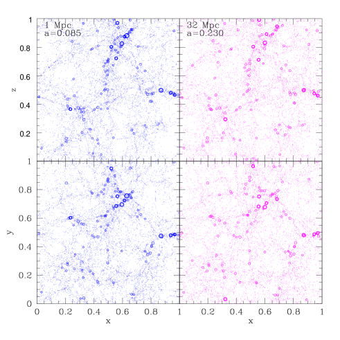
Figure 2: Position of DM halos in the 1 h^-1 Mpc box at $a=0.085$ (left panels) and 32 h^-1 Mpc box at $a=0.23$ (right panels). The circles show the sizes (virial radii) and positions of the 100 most massive halos in the simulation. The 10 most massive halos are shown as thicker circles. The positions of the most massive 10000 halos are shown as points.

2.2 Density Profiles

The density profiles are calculated in three different ways:
(i) Using the list of particles identified as halo members by DENMAX. This means all the bound particles.
(ii) Using, additionally, the particles identified by DENMAX as unbound particles.
(iii) Using all the particles. This includes all the halo satellites and neighbouring halos.
Usually profiles using (i) and (ii) are almost indistinguishable. But the profiles using (iii) look different in the outer parts if the halo is disturbed by accreting satellites. The profiles obtained with method (iii) are used for the analysis as in previous studies. The other profiles are useful to discriminate between isolated halos and halos that are undergoing accretion of massive satellites. One can choose whether to exclude or include in the analysis halos that are undergoing major mergers; either choice does not change the result significantly.

The profiles are shown in dimensionless units: the radii are expressed in number of cells $x$ (the cell size is $\Delta L=L_{box}/256$ in comoving coordinates) and the masses in number of DM particles $N_{p}$. The mass and density of each halo are sampled as a function of the radius, $x$, in shells with constant logarithmic spacing $dx/x=0.01$. The dimensionless circular velocity is more appropriate to compare the profiles since the virial radii are difficult to determine when the halos are not isolated. Moreover, the relative error on the density profile is smaller at radii corresponding to the maximum of the circular velocity since the number of particles per shell at intermediate radii is maximum. Therefore, if the halo profile is not disturbed by accreting satellites, the location and the value of the maximum circular velocity provides the best method to compare halos of different masses. The dimensionless circular velocity is defined as,

$$v_{c}={V_{c}(x)\over V_{c}^{0}}=\sqrt{N_{dm}(x)\over x}$$

where $V_{c}^{0}=(GM_{p}/\Delta L)^{1/2}=7.365\times 10^{-2}(L_{box}/1~{}h^{-1}{\rm Mpc})$ km s^-1. If the slope of the inner density profile is $\rho(r)\propto r^{-\phi}$, the circular velocity has a slope $V_{c}\propto r^{(1-\phi/2)}$. The Poisson error for the density is $\delta\rho/\rho=dN_{p}(x)^{-1/2}$, where $dN_{p}(x)$ is the number of particles in each shell of radius $x$. The error on the mass as a function of the radius is $\delta M_{dm}/M_{dm}(x)=N_{p}(x)^{-1/2}$, where $N_{p}(x)$ is the number of particles in each sphere of radius $x$. The error on the circular velocity is $\delta v_{c}/v_{c}=0.5\delta M_{dm}/M_{dm}$. Table 2 lists the values of useful constants for converting dimensionless units into physical units.

Table 2: Scaling constants.

Lbox	$\Delta L$	Log Mp	$V_{c}^{0}/100$	a
h-1 Mpc	h-1 kpc	h-1 M⊙	km s-1	range
1	3.9	$3.69$	7.26	0.07-0.09
32	125	$8.21$	235.7	0.23-0.3
256	1000	$10.9$	1885	0.9-1.5
1024	4000	$12.7$	7542	$>1000$

3 Results

In Figs. 3-5 (top) the dimensionless circular velocities are shown for the nine most massive halos in the simulations with box sizes $L_{box}=1,32$, and 256 h^-1 Mpc, respectively. The statistical errors, $\delta v_{c}$, on each point are about the sizes of the symbols and therefore are not shown to avoid excessive crowding. I show the profiles obtained using methods (ii) (small dots) and (iii) (large dots). I do not show those obtained using method (i) since they are almost indistinguishable from (ii). I show the fit with a NFW profile obtained by matching the position and value of the maximum of $v_{c}$ and the virial radius (arrow) for the halos that are not severely perturbed by mergers. The points are connected in the range of radii that are reliable: $x_{mi}<x<x_{\Delta}$. Here $x_{\Delta}=2.37(\Delta/178)^{-1/3}(N_{p}/10^{4})^{1/3}$ is the dimensionless virial radius and $x_{mi}$ is the radius that contains a number of particles $N_{p}(x_{mi})\geq 300(\rho(x_{mi})/10^{4})^{1/2}$. This condition ensures that two-body relaxation is not important in flattening the inner profile (see Power et al. (2002) for details on convergence studies). Note that $x_{mi}$ is always larger than twice the Plummer softening length $2\epsilon=0.04$, therefore an incorrect force calculation does not affect the results at those radii. In summary, the sanity checks adopted are as follows.
1) Only radii well above twice the softening length are considered.
2) Only radii that enclose $N_{p}\geq 300(\rho/10^{4})^{1/2}$ particles are considered.
3) No merging halos: profiles (ii) and (iii) give similar results for the value and radius of the maximum circular velocity.
4) The same criteria are adopted for all the simulations with different box sizes, $L_{box}$, and scale factor $a$.

Figs. 3-5 (bottom) show the mean profiles obtained by scaling (shifting in logarithmic scale) the radii to the same $x_{max}=1$ and normalising the maximum of $v_{c}$ to $v_{c}^{max}=1$. Each radial bin, logarithmically spaced, is weighted equally so long as $N_{p}\geq 300(\rho/10^{4})^{1/2}$. Only the halos that are not undergoing a major merger are considered. If all the ten profiles or a different subset of profiles are considered, I find that the resulting mean profile does not change significantly. Also, using the arithmetic or geometric mean does not change the mean profiles. A possible criticism to this method is that the halos analysed are not isolated as in works where a single galaxy is re-simulated with higher resolution. Time-dependent effects could thus produce flatter or steeper cores. For this reason, I present the mean profile at different redshifts (listed in the figure captions). If the halos are not relaxed to their final configuration the mean profiles should differ at different redshifts. Moreover, the increased statistical sample of halos makes the result more robust.

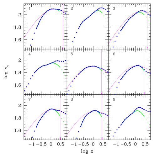
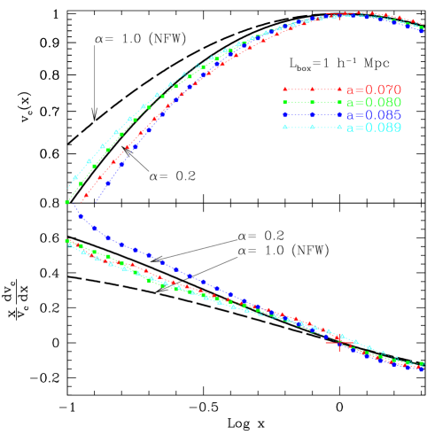
Figure 3: (Top). Dimensionless circular velocity, $v_{c}$, as a function of comoving radius, $x$, for the nine most massive halos in the 1 h^-1 Mpc simulation at $a=0.085$. The points are connected in the interval where the profile is reliable (the arrow indicates the virial radius). The smaller points are obtained using method (ii) (see text) and the thin solid line shows the NFW fit to the profile (for those profiles that are not undergoing major mergers). (Bottom). Normalised mean circular velocity $v_{c}$ (top panel) and its slope (bottom panel) as a function of the normalised radius $x$ of the nine more massive halos in the simulation. The thick dashed line shows the NFW profile and the thick solid line a profile with $\alpha=0.2$. The mean profiles at at $a=0.070,0.080,0.085$ and $0.090$ are shown to ensure that the result is not affected by time dependent effects such as mergers and to increase the statistical significance of the result.

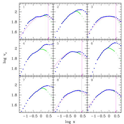
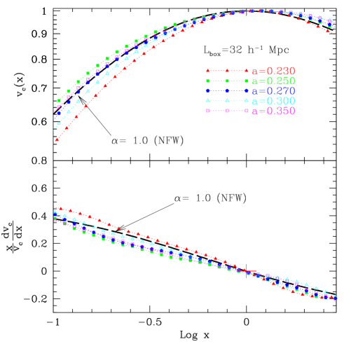
Figure 4: (Top) Same as in Fig. 3 for the 32 h^-1 Mpc box at $a=0.23$. (Bottom) Same as in Fig. 3 for the 32 h^-1 Mpc box at $a=0.23,0.25,0.27$ and $0.30$.

In the 1 h^-1 Mpc simulation (see Fig. 3) the slope of the inner profiles is, on average, flatter (i.e., the circular velocity rises more steeply) than the NFW profile. The typical masses of the halos in this simulation are $M_{dm}\sim 10^{8}$ M_⊙. Even at radii close to $v_{max}$ the circular velocity starts to deviate from the NFW fit. The slope of the outer profile is instead consistent with $\gamma=3$ as in the NFW formula. Note that method (ii) does not attribute several DM particles to the halo, producing an outer profile that decreases more steeply. It is not clear if DENMAX fails not to include those particles or if they effectively do not belong to the halo. The definition of halo boundary (or virial radius) is somewhat arbitrary and time dependent since halos are constantly growing. Especially for small mass halos the flat mass function of the accreting satellites and the short accretion timescale makes it more difficult to define the outer edge of the galaxy. This is also true for dwarf galaxies at $z=0$, even if the accreting satellites are mostly invisible because they do not contain stars. For this reason an “isolated” dwarf galaxy cannot be found or defined in the same way as for massive galaxies for which the mass function of accreting satellites is dominated by halos with masses similar to the host halo. There are halos for which the use of either method (iii) or (ii) gives a different radius where the circular velocity is maximum. Those halos are excluded from the analysis since they are severely disturbed by accreting satellites (but if they were to be included in the analysis, the mean slope would remain flatter than $\alpha=1$). The mean density profiles are best fitted by inner slopes in the range $\alpha\sim 0.4-0.5$, equivalent to mean slopes of the inner circular velocity $\beta\sim 0.75-0.8$.

In the 32 h^-1 Mpc simulation (see Fig. 4) the NFW profile provides a good fit to all the halos that are not severely disturbed by accreting satellites. The typical masses of the halos in this simulation are $M_{dm}\sim 5\times 10^{12}$ M_⊙. The mean density profiles are best fitted assuming inner slopes in the range $\alpha\sim 0.9-1$, equivalent to mean slopes of the inner circular velocity $\beta\sim 0.5-0.55$.

In the 256 h^-1 Mpc simulation (see Fig. 5) the inner density profile slopes appear slightly steeper than predicted by NFW (i.e., flatter circular velocities). Unfortunately, the number of particles in the inner region is barely sufficient to start seeing a discrepancy. A larger number of particles per halo is needed to construct reliable rotation curves at small radii where the discrepancy, expected by extrapolating the reliable part of the rotation curve, should become evident. The typical masses of the halos in this simulation are $M_{dm}\sim 2\times 10^{15}$ M_⊙. The mean density profiles are best fitted by inner slopes in the range $\alpha\sim 1.3-1.4$, equivalent to mean slopes of the inner circular velocity $\beta\sim 0.3-0.35$. In Fig. 5 (bottom), it appears that the slope of the outer profile becomes steeper when $a>1$. For this reason, included in the figure are the best fits for two cases: (i) when the outer slope of the profile is $\gamma\approx 3$ at $a=1.0,1.2$, and (ii) when the slope is $\gamma\approx 4.0$ at $a=1.5,1.7$. This dependence of the outer profile slope on the scale factor becomes more evident in the 1024 h^-1 Mpc simulation and is discussed in the following paragraph.

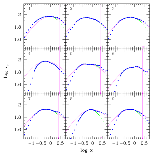
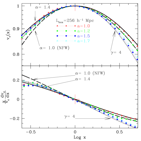
Figure 5: (Top) Same as in Fig. 3 for the 256 h^-1 Mpc simulation at $a=1.0$. (Bottom) Same as in Fig. 3 for the 256 h^-1 Mpc box at $a=1,1.2,1.5$ and $1.7$. The solid and dotted thick lines show two profiles both with $\alpha=1.4$, but with slopes of the outer profile $\gamma=3$ and $\gamma=4$, respectively.

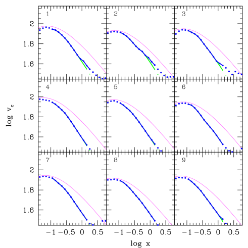
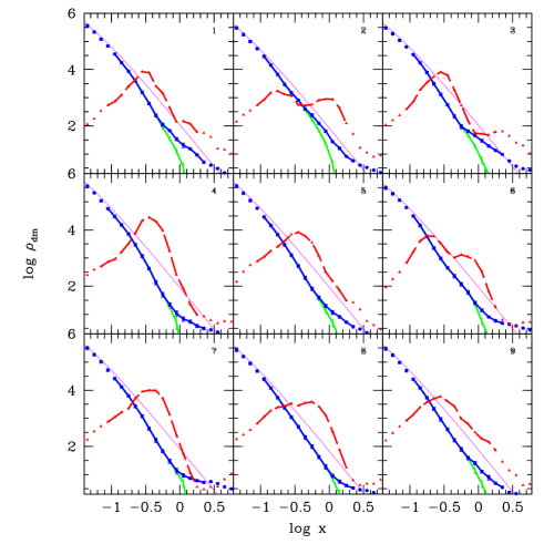
Figure 6: (Top) Same as in Fig. 3 for the 1024 h^-1 Mpc simulation at $a=10$. (Bottom) Density profile (solid lines) and slope of the density profile (dashed lines) for the 1024 h^-1 Mpc simulation at $a=10$. The thin solid line is the fit with the NFW profile. The outer slope of the density profile is $\gamma\approx 4$, steeper than in the NFW profile. This is probably caused by the accelerating universe.

In Fig. 6 (top), the dimensionless circular velocities are shown for the nine most massive halos in the simulation with box size $L_{box}=1024$ h^-1 Mpc at $a=10$. The number of particles in these halos is too small for measuring the slope of the inner profile but it is evident that the outer slope is steeper than the NFW profile. Fig. 6 (bottom) shows the density profiles (solid lines) and slope of the density profiles (dashed lines) for the nine more massive halos in the same simulation. The outer density profile has a slope $\gamma\sim 4$. At $a=2.3$ the slope is $\gamma\sim 3.5$ and increases to $\gamma\sim 4$ when the scale factor is $a=4,10,100$ and 1000. The physical explanation of this result is likely to be related to the expansion rate of the universe. When $\Omega_{\Lambda}(z)\sim 0$ at $a\lower 2.15277pt\hbox{$\;\buildrel<\over{\sim}\;$}0.5$ the universe is decelerating and $\gamma\sim 3$. As $a$ increases to $a\lower 2.15277pt\hbox{$\;\buildrel>\over{\sim}\;$}1$ the universe starts inflating (at $a=2$, $\Omega_{\Lambda}\sim 0.95$ in a flat universe) and the slope of the outer profiles becomes $\gamma\sim 4$. It is possible that even at $z=0$ the outer profile of recently virialized clusters is slightly steeper than $\gamma=3$. According to the aforementioned interpretation, the observation of a steep outer profile in nearby clusters would indicate that the universe is accelerating (see also the results of Subramanian et al. (2000) for low density universes). In § 4 I show that for the halo profiles in this simulation the radii, $r_{max}$, where the circular velocity is maximum, decrease with increasing scale factor, consistent with the predictions assuming an inner slope of the density profile $\alpha\sim 1.5$.

3.1 Radiative Feedback Effects on the DM profile

Fig. 7 shows the mean $v_{c}$ for the nine most massive halos in the simulation 256L1p3 presented by Ricotti et al. (2002b) at $a=0.075$ and $a=0.090$. This simulation attempts to simulate realistically the formation of the first galaxies in the universe modeling radiative feedback effects in the early universe. The parameters of the simulation are the same as in the 1 h^-1 Mpc simulation presented in this work. But in addition to DM particles it includes gas dynamics, star formation using a Schmidt-Law, metal enrichment from star formation and radiative transfer. Radiative feedback effects produced by UV radiation emitted by the first stars are calculated following the molecular processes involving H₂ formation, destruction and cooling. From the results presented in this work it appears that radiative feedback processes are not responsible for the flattening of the DM profile in small-halos. The slopes of the inner profile of the halos in this simulation are similar to the corresponding N-body simulation, or perhaps slightly steeper.

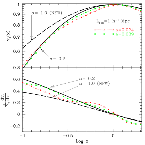
Figure 7: Same as in Fig. 3 (Bottom) for the 1 h^-1 Mpc simulation presented by Ricotti et al. (2002b) at $a=0.075$ and $0.090$ (see text).

4 Constant concentration DM profiles

In comoving coordinates, $r$, all of the simulated halos in this work can be fitted by a profile with the form (cf., Zhao, 1996)

$$\rho_{dm}(X)\propto{1\over X^{\alpha}(1+X)^{\gamma-\alpha}},$$ (1)

where $X=c_{\Delta}r/r_{\Delta}$, $r_{\Delta}$ is the comoving virial radius, $\alpha=\alpha(M_{dm})$ is a function of the halo mass, $M_{dm}$, and $c_{\Delta}\sim 7$ is the concentration parameter that, as I will show, is a constant. In physical coordinates, $R$, it is simply $X=c_{\Delta}R/R_{\Delta}$, where $R_{\Delta}=(1+z)^{-1}r_{\Delta}$ is the virial radius. Given the initial power spectrum of density perturbations, the parameter $\alpha$ is a function of the halo mass only. The values found in this work agree with the predictions of Subramanian et al. (2000) (see Fig. 8). An acceptable fit to the theoretical value of $\alpha$ for the case of the $\Lambda$CDM cosmology, adopted in this work, has the form $\alpha\approx 1.3+(M_{dm,14}^{1/6}-1)/(M_{dm,14}^{1/6}+1)$, where $M_{dm,14}=M_{dm}/(3\times 10^{14}$ M_⊙). This fit is five percent accurate for masses $10^{6}\lower 2.15277pt\hbox{$\;\buildrel<\over{\sim}\;$}M_{dm}/M_{\odot}\lower 2.15277pt\hbox{$\;\buildrel<\over{\sim}\;$}10^{18}$.

The logarithmic slope, $\gamma$, of the outer parts of the halo appears to depend on the acceleration of the universe: when the scale parameter is $a\lower 2.15277pt\hbox{$\;\buildrel<\over{\sim}\;$}1$, the slope is $\gamma\approx 3$ as in the NFW profile, but is $\gamma\approx 4$ at $a>1$ when $\Omega_{\Lambda}\sim 1$ and the universe is inflating. Equation (1) is normalised imposing the condition that the integrated mass inside the virial radius is $m_{dm}(X=c_{\Delta})=M_{dm}$ (see appendix A). The comoving virial radius is defined as

$$r_{\Delta}\equiv(32~{}{\rm kpc})\left({\Delta\over 178}\right)\left(M_{dm}\over 10^{6}M_{\odot}\right)^{1/3},$$

to satisfy the relation $M_{dm}=(4\pi/3)\rho_{0}\Delta r_{\Delta}$, where $\Delta$ is the mean overdensity of the halo and $\rho_{0}$ is the mean DM density at $z=0$. $\Delta$ depends on the cosmology since it is related to the mean overdensity and the time it takes for a density perturbation to stop expanding with the universe and “turn around,” starting the collapse. According to the simple top-hat spherical collapse approximation, $\Delta\approx 178\Omega_{0}(z)^{0.45}$ for a flat universe with a cosmological constant (Eke et al., 1998).

I now explain why this profile has the property of a constant concentration parameter. The changing slopes of the inner and outer parts of the profile mimics the variation of the concentration parameter in the NFW profile, shifting the value of the radius, $r_{max}$, where the circular velocity reaches its maximum value. For the NFW profile (i.e., for $\alpha=1$) $r_{\Delta}/r_{max}=c_{\Delta}^{NFW}/2.16$, therefore the location of $r_{max}$ with respect to the virial radius is inversely proportional to the concentration parameter. In the general case

$${r_{\Delta}\over r_{max}}={c_{\Delta}\over f(\alpha,\gamma)}.$$ (2)

The location of the maximum circular velocity depends on the inner and outer profile slopes and on the concentration parameter. In appendix A I show that a good approximation for the function $f(\alpha,\gamma)$ is $f\approx(4/\gamma)^{2.68}(2-\alpha)$. In Fig. 8 it can be seen that the values of $r_{\Delta}/r_{max}$ (circles), for all the simulations in this work (listed in Table 1), agree with equation (2), assuming constant concentration parameter $c_{\Delta}=7$. Moreover the values of $\alpha$ (triangles) are in good agreement with the theoretical relationship proposed by Subramanian et al. (2000), $\alpha=(9+3n)/(5+n)$ (dashed line), where $n$ is the effective slope of the power spectrum. The solid and open circles show $r_{\Delta}/r_{max}$ measured in profiles with $\gamma=3$ (i.e., at $a<1.2$) and with $\gamma>3$, respectively. The solid and dash-dotted lines show $r_{\Delta}/r_{max}$ given by equation (2) using the theoretical value of $\alpha$ (shown by the dashed line), $\gamma=3$ and $\gamma=3.5-4$, respectively. In the 1024 h^-1 Mpc box simulation I find that $\gamma\sim 4$. The inner slope of the profile cannot be measured because of the small number of particles in the inner regions. But the measured values of $r_{\Delta}/r_{max}$ are consistent with values of the inner slope $\alpha\sim 1.5$, predicted by the theory.

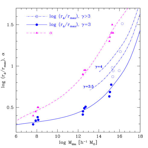
Figure 8: $r_{\Delta}/r_{max}$ (circles) and $\alpha$ (triangles) for the simulations listed in Table 1 as a function of the halo DM mass $M_{dm}$. The open circles show $r_{\Delta}/r_{max}$ when $\gamma>3$ at $a>1$. The dashed line shows the theoretical value of $\alpha$ (see text). The solid and dash-dotted lines show $r_{\Delta}/r_{max}$ for the profile given in Eq. (1) using $\gamma=3$ and $\gamma=4$, respectively.

5 Discussion

The results presented in this work and their interpretation seem to disagree with most previously published work, although the simulations presented here are not of substantially higher resolution than those in the literature. In this section I analyse the discrepancies with previous works and point out that the results do not disagree strongly with most previous works, save for the 1 h^-1 Mpc simulation. The result of the 1 h^-1 Mpc simulation cannot be compared with previous works since a similar simulation has not been performed before. The joint analysis of the three simulations with $L_{box}=1,32$ and 256 h^-1 Mpc suggests that the slope of the inner part of the DM profile depends on the power spectrum of linear perturbation. This interpretation of the results disagrees with the common view of universality of DM profiles, although several groups have found results that contrast with this idea, both in the context of galactic dynamics (Nipoti et al., 2003, e.g.,) and cosmology (Syer & White, 1998; Kravtsov et al., 1998; Jing & Suto, 2000; Jing, 2000). Here I identify and summarise three possible reasons why the present results differ from a large number of published work on N-body simulations.

1. The profiles of halos with typical masses resolved by the 1 h^-1 Mpc simulation have not been analysed before. This simulation is equivalent to a scale free simulation with linear power spectrum $P(k)\propto k^{n}$ with $n=-2.7$ and Einstein-de Sitter cosmology, since at $z>2$ the cosmological constant contribution is negligible. Previous works have studied scale free simulations with power spectrum index $n\geq-2$. For instance Cole & Lacey (1996) studied the $n=0,-1,-2$ cases and Navarro et al. (1997) the $n=0,-0.5,-1,-1.5$ cases. The simulations in those works have the same resolution as in the present study. Their results do not contrast with the findings of this work because when $n\lower 2.15277pt\hbox{$\;\buildrel>\over{\sim}\;$}-2$ the inner slope of DM profiles is also $\alpha\approx 1-1.5$. But, as mentioned, the resolution of the simulations (about $10^{4}-10^{5}$ particles per halo) is marginally sufficient to discern between $\alpha\sim 1$ and $\alpha\sim 1.5$. The $n=-2.7$ case is markedly different from the others since it corresponds to a scenario in which all mass perturbations become non-linear at about the same time (an index $n<-3$ would correspond to the top-down formation scenario, in which small mass halos form after the large ones). For this reason, I believe that the result found analysing the 1 h^-1 Mpc simulation is new and complements previous studies.

2. Interpretation of the results. Theoretically it is unclear what determines the slope of the inner DM profiles. Some works argue that the slope depends on the power spectrum of initial perturbations (Syer & White, 1998; Subramanian et al., 2000), others argue that the slope tends asymptotically to a steep slope $\alpha\sim 1-2$ (Alvarez et al., 2003; Dekel et al., 2003). Recent still unpublished high-resolution N-body results from Navarro and collaborators show that the inner slope does not converge to $\alpha=1$ but the slope slowly flattens to $\alpha\lower 2.15277pt\hbox{$\;\buildrel<\over{\sim}\;$}1$. This result contrasts with most aforementioned semi-analytical results indicating that physical processes that determine the density profile of DM halos and their time evolution are not well understood.

   The halos analysed in the present work are the most massive halos at a given redshift. For this reason they are recently virialized halos with different masses, compared after about the same number dynamical times from their formation. The halos analysed in high-resolution N-body studies are usually chosen to be “isolated”: halos that did not experience “recent” major mergers. Therefore, depending on their mass, their age from the virialization differs greatly at $z=0$. Semi-analytical works study the equilibrium profile of halos given an accretion history. The different evolutionary states of the halos studied in literature could explain the discrepancies in the results if the time scale to reach the equilibrium configuration is long compared to the accretion time. I find that the halo profile depends on the accretion history. But it is possible that this is true only during a transient period of time, before the halo relaxes to a different equilibrium configuration. This concern is especially valid for the 1 h^-1 Mpc simulation since in a scale free simulation with $n\sim-2.7$ the halos continuously accrete satellites. The result is therefore statistically significant at redshift about 10 but the shallow slope of the profiles might not survive to redshift $z=0$. Even if the shallow profiles are transient, depending on the time scale to reach the equilibrium configuration, the result at $z=10$ might suggest a reason for why not all dwarf galaxy halos at $z=0$ present shallow cores. According to the work of Dekel et al. (2003), substructure is not tidally striped but instead is compressed when the halo profile is shallow. Therefore substructure could survive undigested for quite a long time. Moreover even at $z=0$, small mass halos, due to their larger number density, are expected to capture dark satellites of non-negligible mass with higher frequency than larger mass halos. Further work is needed, and is currently in progress (Ricotti & Wilkinson, 2003), to extend the result of the present work from redshift $z=10$ to redshift $z=0$. The aim of this study is to understand if the flat profiles at $z=10$ are in a stable configuration that would survive for a Hubble time and if the profiles are consistent with the observed flat cores of dSph galaxies in the local group. Preliminary results show that the dynamical state of the halos is stable and the inner profiles remain flat for $20$ Grys if the halo is evolved in isolation.

   To further support the case for a dependence of the inner profile on the mass of the halos I show that flat inner profiles are associated with an almost isotropic velocity dispersion of DM particles while steeper profiles have a velocity dispersion slightly biased in the radial direction. This result is shown in Fig. 9. The lines show the parameters $\beta=1-\sigma^{2}_{\theta}/\sigma^{2}_{r}$ (dashed lines) and $\beta^{*}=1-\langle v_{\theta}^{2}\rangle/\langle v_{r}^{2}\rangle$ (solid lines) as a function of the scaled radius $x=r/r_{max}$, where $r_{max}$ is the radius where the circular velocity is maximum. Here, $\sigma^{2}_{\theta}=\langle v_{\theta}^{2}\rangle-\langle v_{\theta}\rangle^{2}$ and $\sigma^{2}_{r}=\langle v_{r}^{2}\rangle-\langle v_{r}\rangle^{2}$, where $v_{r}$ is the radial velocity and $v_{\theta}$ is the tangential velocity. The $\beta$ parameter measures the degree of anisotropy of the velocity dispersion: $\beta=0$ corresponds to an isotropic velocity dispersion, $\beta<0$ to a tangentially biased velocity dispersion and $0<\beta<1$ to a radially biased velocity dispersion. The lines from top to bottom show the mean value of $\beta$ and $\beta^{*}$ for the 9 most massive halos in the 256 h^-1 Mpc, 32 h^-1 Mpc and 1 h^-1 Mpc simulations. The shallow inner DM profiles in the 1 h^-1 Mpc simulation have almost isotropic velocity dispersion. Steeper DM profiles in the 32 h^-1 Mpc and 256 h^-1 Mpc simulations have a velocity dispersion slightly biased in the radial direction. This result is consistent with the analytical expectations based on the solution of the Jeans equations in spherical systems.

   

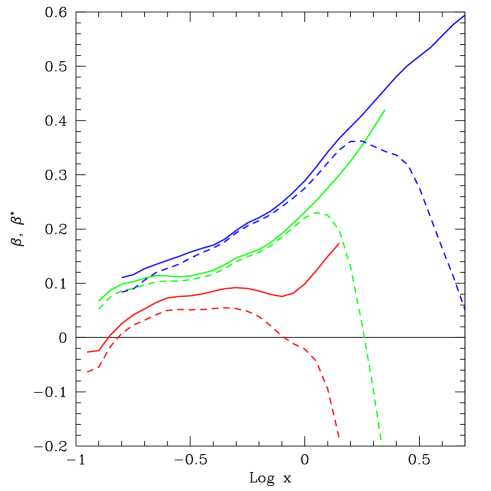
   Figure 9: $\beta=1-\sigma_{\theta}^{2}/\sigma_{r}^{2}$ (dashed line) and $\beta^{*}=1-\langle v_{\theta}^{2}\rangle/\langle v_{r}^{2}\rangle$ (solid lines) as a function of the scaled radius $x=r/r_{max}$. The lines from top to bottom show the mean value of $\beta$ and $\beta^{*}$ for the 9 most massive halos in the 256 h^-1 Mpc, 32 h^-1 Mpc and 1 h^-1 Mpc simulations (shown in the top panels of Figs. 3-5). The shallow inner DM profiles in the 1 h^-1 Mpc simulation have almost isotropic velocity dispersion ($\beta\sim 0$). Steeper DM profiles in the 32 h^-1 Mpc and 256 h^-1 Mpc simulations have a velocity dispersion slightly biased in the radial direction (i.e., $\sigma_{r}>\sigma_{\theta}$).

3. Method and analysis of the results In this paper I present statistical results without preselecting the halos to re-simulate with higher resolution as has been done in previous studies. In order to compare simulations with observations a statistically significant sample should be analysed. Halos that did not reach an asymptotic equilibrium configuration (if they exist) or halos presenting substructures produced by recent mergers should be included in the analysis if they appear to be statistically significant. Especially if there is not an easy way to determine the dynamical stage of a halo because the accreting substructure is invisible (small halos at $z=0$ should accrete mostly dark halos), understanding what fraction of dark halos of a given mass is in a transient configuration is relevant to solve the problem of the DM cores observed in a fraction of galaxies at low redshift.

   As expected the halos studied in this work show substantial substructure. 3D images of the halos show that numerous satellites are present, independently of the halo mass. Perhaps in small mass halos substructure can survive “undigested” closer to the halo cores. Nevertheless, in most cases, this does not affect the approximately spherical symmetry of the halos and the determination of the halo centres. The halo centres are calculated, using DENMAX, as the minimum of the gravitational potential. I also calculate the centres as the maximum of halo density and as the centre of mass of bound particles. The halo centres calculated using those alternative definitions are practically coincident and choosing either of them does not change the profiles. Exceptions are profile 8 in the 1 h^-1 Mpc simulation and profile 4 in the 256 h^-1 Mpc simulation that have maximum density centres offset by 2$\epsilon$, where $\epsilon$ is the Plummer softening parameter.

   In this work the inner slope of the profiles and the core radii are determined fitting the circular velocities instead of the density profiles. This procedure partially remove the degeneracy between the slope $\alpha$ of the inner profile and the core radius $r_{s}$. This is illustrated in Fig. 10, which shows the maximum likelihood estimate of the parameters $\alpha$ and $r_{s}$ fitting the density profile (left) or the circular velocity (right). The $1\sigma,2\sigma$ and $3\sigma$ confidence contours are shown assuming constant relative errors on the density and circular velocity in each logarithmically spaced radial bin.

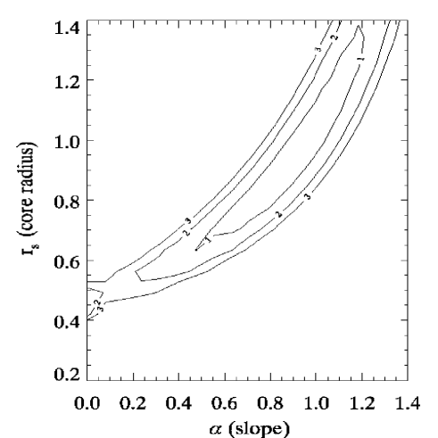
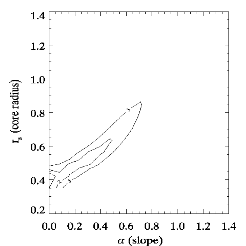
Figure 10: Maximum likelihood estimate of the core radius, $r_{s}$, and inner slope, $\alpha$. The $1\sigma,2\sigma$ and $3\sigma$ confidence contours are shown. The degeneracy between the core radius and inner slope when the density profile is fitted with the generalised profile given in Eq. (1) (left panel) can be partially broken fitting the circular velocity (right panel).

6 Conclusions

Two main problems faced by CDM cosmologies are related to the properties of small mass galaxies. Namely, (i) the number of visible galactic satellites (dwarf galaxies) in the Local Group is smaller than predicted by N-body simulations (Moore et al., 1999; Klypin et al., 1999) and (ii) the flatness of the DM cores in dwarf and LSB galaxies is not reproduced by N-body simulations. The first problem can be solved by including radiative feedback effects (Chiu et al., 2001; Ricotti et al., 2002b) in cosmological simulations. Galaxies with masses $M_{dm}\lower 2.15277pt\hbox{$\;\buildrel<\over{\sim}\;$}10^{8}-10^{9}$ M_⊙ are too small to retain the gas that is photoevaporated by stars or by the ionising background after reionization. Consequently, the luminosity of most dwarf galaxies is predicted to be too low to be detected (i.e., the mass-to-light ratio should increase for halos with smaller masses) or zero for very small mass halos. Here I have shown results of N-body simulations suggesting that the second problem might not contradict the predictions of CDM cosmologies. But further investigation is needed to understand if the dwarf galaxies showing shallow DM profiles at $z\sim 10$ (e.g., just after the time when most of the dwarf galaxies formed) are in a configuration that will survive unchanged until redshift $z=0$. In summary the main findings of this work are:

• The slope, $\alpha$ of the inner profile of DM halos is determined by the mass function of the accreting substructure (i.e., the initial power spectrum of initial perturbations). Dwarf galaxies have on average flatter DM cores, and clusters, steeper cores than galaxies similar to the Milky Way for which the NFW profile is a good fit to the halo density profile.

• The logarithmic slope, $\gamma$, of the outer parts of the halo appears to depend on the acceleration of the universe: when the scale parameter is $a\lower 2.15277pt\hbox{$\;\buildrel<\over{\sim}\;$}1$, $\gamma\approx 3$ as in the NFW profile, but $\gamma\approx 4$ at $a>1$ when $\Omega_{\Lambda}\sim 1$ and the universe is inflating.

• A density profile in the form $\rho_{dm}\propto X^{-\alpha}(1+X)^{-\gamma+\alpha}$, where $X=c_{\Delta}r/r_{\Delta}$, $\alpha$ is a function of the halo mass ($\alpha\approx 1.3+[M_{dm,14}^{1/6}-1]/[M_{dm,14}^{1/6}+1]$, where $M_{dm,14}=M_{dm}/[3\times 10^{14}$ M_⊙]) and $\gamma\sim 3$ (but $\gamma\sim 4$ if $\Omega_{\Lambda}\sim 1$), can fit all the profiles from dwarfs to superclusters with constant concentration parameter $c_{\Delta}\simeq 7$. This provides a physical explanation for the variation of the concentration parameter in the NFW profile as a function of the halo mass: the changing slopes mimic the variation of the concentration parameter by shifting the radius where the circular velocity reaches its maximum value.

• The dependence of $\alpha$ on the mass of the halo, and therefore on the slope of the power spectrum, $n$, agrees with the theoretical expectation $\alpha=(9+3n)/(5+n)$, derived assuming that “undigested” satellites determine the halo structure in the inner regions (Subramanian et al., 2000). Note that if the DM halo develops a flat core, the chance for accreting satellites to survive tidal disruption is larger (Dekel et al., 2003).

The shape of the profiles for a given mass and redshift present significant statistical variations. This can be attributed to two factors. Firstly, galaxies are not isolated entities and especially at high redshift are severely disturbed by neighbouring satellites or by undergoing major mergers. This produces irregularities in the azimuthally averaged density profile. Secondly, the accretion history of satellites has statistical variation and depends on the local environment. A dwarf galaxy forming at high redshift from a large $\sigma$ peak of the power spectrum of initial perturbations (the type of galaxy simulated in this work) could have an inner profile different from the same mass galaxy forming at lower redshift from a smaller $\sigma$ perturbation. Also, the slope of the profile could differ if a galaxy forms in a void or in an overdense region, even for galaxies with similar masses and radii.

I have identified three main reasons to explain why previous studies (e.g., Eke et al., 2001; Moore et al., 1999) found that the inner slope of the DM profiles are not determined by the power spectrum or accretion history (but see also Syer & White (1998); Kravtsov et al. (1998); Jing & Suto (2000); Jing (2000) for a different point of view). (i) The profiles of halos with typical masses resolved by the 1 h^-1 Mpc simulation have not been analysed before. (ii) The dynamical state of the the halos at $z=10$ might be different at $z=0$. But there are not published high-resolution simulations for dwarf-size halos ($M_{DM}\sim 10^{8}$ M_⊙) at $z=0$. The classic results of Cole & Lacey (1996); Navarro et al. (1997) are based on the same type of simulations presented here. (iii) Most of the computational efforts have focused on simulating a single galaxy-size or cluster-size halo with mass $M_{dm}\lower 2.15277pt\hbox{$\;\buildrel>\over{\sim}\;$}10^{12}$ M_⊙ at $z=0$ with higher resolution (about $10^{6}$ particles per halo) than in this study. Such a large number of particles is required to study the profile in the very inner regions of the halo. But the task of achieving reliable profiles with such a high spatial resolution is sensitive to numerical integration errors and requires careful resolution studies (Power et al., 2002); perhaps this is a reason for the disagreement between groups, using different codes, on the slope of the inner profile. In this work I find that the shape of the DM profiles present significant scatter around the mean. It is, therefore, important to analyse a significant statistical sample of halos in order to measure the mean profile. Works where a single halo is re-simulated with higher resolution are affected by a bias, difficult to control, determined by the criteria for picking the halos to re-simulate. Finally, the fitting method could be important as well for the results. The degeneracy between the slope of the inner profile and the value of the core radius is more easily broken fitting the circular velocities instead of the density profiles. This is because the radius where the circular velocity is maximum is univocally determined by the value of the core radius, $r_{s}$ (for the NFW profile is $r_{max}=2.16r_{s}$). The halo profiles at any redshift and mass, when renormalised matching the values and radii of the maximum circular velocities, have to be identical if their profiles can be all fitted by the NFW profile.

Moore et al. (1999) find steep profiles in cluster size halos ($\alpha\sim 1.5$), in agreement with the results of this work. The results of this work also agree with the classic NFW result for Milky Way size galaxies but not with Moore et al. (1999) for halos with the same mass. In this work the spatial resolution is not as large as in the aforementioned studies, therefore I cannot study the slope of the DM profile in the very centre of the halos. Nevertheless, I find evidence for disagreement with the NFW predictions even at relatively large radii. Perhaps this new result has been found because it is the first time that a simulation of halos with masses typical of dwarf galaxies and mass resolution $M_{p}\sim 10^{3}$ M_⊙ has been performed. The result for the cluster size halos could also be understood with similar reasoning (i.e., the cluster masses are larger than in previous studies: $M_{dm}\sim 10^{15}-10^{16}$ M_⊙). The steeper core density profile found in clusters may not be as evident as the flatter core found in dwarf galaxies but, combined with the result for normal galaxies, the findings from the three simulations strengthen the case for an inner slope that changes with the mass of the halos.

I conclude this work with two final remarks:

• According to the scaling relation $\alpha=(9+3n)/(5+n)$, the inner slope of DM profile of dwarf galaxies is more sensitive to the power spectrum index, $n$, than more massive galaxies: $\delta\alpha=1.5\delta n$ if $n\sim-3$. A tilt $\delta n\approx 0.2$ in the initial power spectrum should produce a variation $\delta\alpha\approx 0.3$ of the inner slope of the DM profile.

• The best place to look for the effects of the cosmological constant is the outer profile of clusters and superclusters at low redshift. The prediction is for a slope steeper than $\gamma=3$. Perhaps gravitational lensing studies could be useful in this regard.

ACKNOWLEDGEMENTS

M.R. is supported by a PPARC theory grant. Research conducted in cooperation with Silicon Graphics/Cray Research utilising the Origin 3800 supercomputer (COSMOS) at DAMTP, Cambridge. COSMOS is a UK-CCC facility which is supported by HEFCE and PPARC. I would like to thank Jerry Ostriker for his valuable comments on the draft and exciting discussions.

Appendix A Generalised Profile

The comoving virial radius, $r_{\Delta}$, here is defined as the radius where the halo mean overdensity is $\Delta$, i.e., $M_{dm}\equiv(4\pi/3)\rho_{0}\Delta r_{\Delta}^{3}$. Here $M_{dm}$ is the mass of the halo, $\rho_{0}$ is the mean DM density at $z=0$ and $\Delta\approx 178$ if $\Omega(z)=1$. A density profile with inner slope $\alpha$, and outer slope $\gamma$, can be written in the form

$$\rho_{dm}(r)={\rho_{0}\Delta\delta_{(c,\alpha,\gamma)}\over X^{\alpha}(1+X)^{\gamma-\alpha}}$$

where $X=r/r_{s}$, $r_{s}=r_{\Delta}/c_{\Delta}$ is the core radius and $\delta_{(c,\alpha,\gamma)}$ is a normalisation constant. The NFW profile has $\alpha=1$ and $\gamma=3$. The mass enclosed inside the radius, $X$, is

$$\begin{split}m_{dm}(X)=4\pi\rho_{0}\Delta\delta_{(c,\alpha,\gamma)}r_{s}^{3}\int_{0}^{X}{y^{g}\over(1+y)^{\gamma-\alpha}}{dy\over y}=\\ 4\pi\rho_{0}\Delta\delta_{(c,\alpha,\gamma)}r_{s}^{3}\left({X^{g}\over g}\right){{}_{2}F_{1}}(g;\gamma-\alpha;g+1;-X)\end{split}$$ (3)

where $g=(3-\alpha)$ and ${}_{2}F_{1}$ is the hypergeometric function. If $\gamma=3$, the hypergeometric function simplifies as

$${{}_{2}F_{1}}(g;g;g+1;-X)=g\sum_{n=0}^{\infty}{{\cal B}(n;g)\over(g+n)n}(-X)^{n},$$

where $\cal B$ is the beta function. When $\alpha=1$ and $\gamma=3$ (NFW profile) equation (3) can be integrated analytically and the solution is

$$m_{dm}(X)={4\pi\over 3}\rho_{0}\Delta\delta_{c}^{NFW}r_{s}^{3}\left[\ln(1+X)-{X\over 1+X}\right].$$

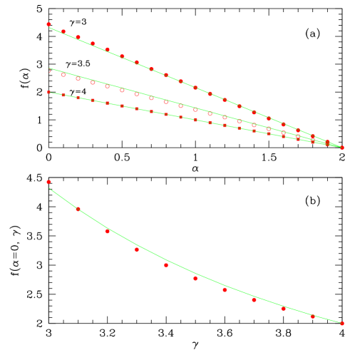
Figure 11: (a) $f(\alpha,\gamma)=r_{max}/r_{s}$ as a function of $\alpha$ for $\gamma=3$ (circles), $\gamma=3.5$ (open circles), and $\gamma=4$ (squares). The solid lines show the fit to the numerical solution. (b) $f(\alpha=0,\gamma)=r_{max}/r_{s}$ as a function of $\gamma$. The solid lines show the fit, $f=(4/\gamma)^{2.65}(2-\alpha)$, to the numerical solution.

The normalisation constant $\delta_{(c,\alpha,\gamma)}$ is such that $m_{dm}(X=c_{\Delta})=M_{dm}$. For the NFW profile, $\delta_{c}^{NFW}=c_{\Delta}^{3}/[\ln(1+c_{\Delta})-c_{\Delta}/(1+c_{\Delta})]$. In the general case equation (3) has to be evaluated numerically. If $\gamma=3$, analytical solutions exist for $\alpha=0,0.5,1,1.5$ and 2:

$${}_{2}F_{1}(-X)=\begin{cases}{3\over X^{3}}\left[-{(1+3X/2)X\over(1+X)^{2}}+\ln{(1+X)}\right],~{}~{}\text{if}~{}\alpha=0\\ {5\over X^{5/2}}\left[-{(1+4X/3)X^{1/2}\over(1+X)^{3/2}}+{\rm ArcSinh}(X^{1/2})\right],~{}~{}\text{if}~{}\alpha=0.5\\ {3\over X^{3/2}}\left[-\left({X\over 1+X}\right)^{1/2}+{\rm ArcSinh}(X^{1/2})\right]~{}~{}\text{if}~{}\alpha=1.5\\ {\ln(1+X)\over X},~{}~{}\text{if}~{}\alpha=2\end{cases}$$

If $\gamma=4$ an analytical solution exists for a generic $\alpha$:

$${}_{2}F_{1}(-X)=\left({1+X\over X}\right)^{\alpha}[1-3(1+X)^{-1}+3(1+X)^{-2}-(1+X)^{-3}].$$

The circular velocity is defined as

$$V_{c}(X)=\sqrt{m_{dm}(X)\over Xr_{s}}.$$ (4)

For the NFW profile equation (4) has a maximum $V_{c}^{max}\propto r_{\Delta}$ at $r_{max}=2.16r_{s}$. For a fixed value of $r_{\Delta}$, $V^{max}_{c}$ depends weakly on $c_{\Delta}$, and $r_{max}$ is inversely proportional to $c_{\Delta}$. In the general case, $r_{max}=f(\alpha,\gamma)r_{s}$ and must be calculated numerically. In Fig. 11(a) I show the numerical solution and a simple fit to $f(\alpha,\gamma)=r_{max}/r_{s}$ as a function of $\alpha$ for $\gamma=3,3.5$ and 4. If $\alpha=0$ the maximum, $f$, of $v_{c}$ can be found solving the equation

$$2[1-(1+f)^{\gamma}]+(\gamma-1)f\left[(\gamma-2)^{2}f^{2}+\gamma f+{2\gamma\over\gamma-1}\right]=0.$$

If $\gamma=4$ the solution is $f=2$, but in general the solution has to be evaluated numerically. The simplest fit to the numerical solution, shown in Fig. 11(b), is given by $f=(4/\gamma)^{2.68}$. Using this fit in conjunction with the previous for $f(\alpha,3)$, a general fitting formula is found to be

$${r_{max}\over r_{s}}=f(\alpha,\gamma)\approx(4/\gamma)^{2.68}(2-\alpha),$$ (5)

which is at least 5 percent accurate in the parameter interval $0<\alpha<2$ and $3<\gamma<4$.

References

- Alvarez et al. (2003) Alvarez M. A., Ahn K., Shapiro P. R., 2003, in M. Reyes E. V.-S., ed., ”The Eighth Texas-Mexico Conference on Astrophysics” RevMexAA SC
- Bertschinger (1995) Bertschinger E., 1995, COSMIC, GC-3 report, (astro-ph/9506070)
- Bertschinger & Gelb (1991) Bertschinger E., Gelb J. M., 1991, Computers in Physics, 5, 164
- Bode et al. (2001) Bode P., Ostriker J. P., Turok N., 2001, ApJ, 556, 93
- Borriello & Salucci (2001) Borriello A., Salucci P., 2001, MNRAS, 323, 285
- Chiu et al. (2001) Chiu W. A., Gnedin N. Y., Ostriker J. P., 2001, ApJ, 563, 21
- Cole & Lacey (1996) Cole S., Lacey C., 1996, MNRAS, 281, 716
- de Blok & Bosma (2002) de Blok W. J. G., Bosma A., 2002, A&A, 385, 816
- de Blok et al. (2001) de Blok W. J. G., McGaugh S. S., Bosma A., Rubin V. C., 2001, ApJ, 552, L23
- Dekel et al. (2003) Dekel A., Devor J., Hetzroni G., 2003, MNRAS, in press (astro-ph/0204452)
- Eke et al. (1998) Eke V. R., Navarro J. F., Frenk C. S., 1998, ApJ, 503, 569
- Eke et al. (2001) Eke V. R., Navarro J. F., Steinmetz M., 2001, ApJ, 554, 114
- Gnedin & Bertschinger (1996) Gnedin N. Y., Bertschinger E., 1996, ApJ, 470, 115+
- Huss et al. (1999) Huss A., Jain B., Steinmetz M., 1999, ApJ, 517, 64
- Jing (2000) Jing Y. P., 2000, ApJ, 535, 30
- Jing & Suto (2000) Jing Y. P., Suto Y., 2000, ApJ, 529, L69
- Klypin et al. (1999) Klypin A., Kravtsov A. V., Valenzuela O., Prada F., 1999, ApJ, 522, 82
- Kravtsov et al. (1998) Kravtsov A. V., Klypin A. A., Bullock J. S., Primack J. R., 1998, ApJ, 502, 48
- Moore et al. (1998) Moore B., Governato F., Quinn T., Stadel J., Lake G., 1998, ApJ, 499, L5
- Moore et al. (1999) Moore B., Quinn T., Governato F., Stadel J., Lake G., 1999, MNRAS, 310, 1147
- Navarro et al. (1996) Navarro J. F., Frenk C. S., White S. D. M., 1996, ApJ, 462, 563
- Navarro et al. (1997) Navarro J. F., Frenk C. S., White S. D. M., 1997, ApJ, 490, 493
- Nipoti et al. (2003) Nipoti C., Londrillo P., Ciotti L., 2003, MNRAS, accepted
- Power et al. (2002) Power C., Navarro J. F., Steinmetz M., 2002, The inner, (astro-ph/0201544) submitted
- Ricotti et al. (2002a) Ricotti M., Gnedin N. Y., Shull J. M., 2002a, ApJ, 575, 33
- Ricotti et al. (2002b) Ricotti M., Gnedin N. Y., Shull J. M., 2002b, ApJ, 575, 49
- Ricotti & Wilkinson (2003) Ricotti M., Wilkinson M. I., 2003, in preparation
- Salucci & Burkert (2000) Salucci P., Burkert A., 2000, ApJ, 537, L9
- Spergel & Steinhardt (2000) Spergel D. N., Steinhardt P. J., 2000, Physical Review Letters, 84, 3760
- Subramanian et al. (2000) Subramanian K., Cen R., Ostriker J. P., 2000, ApJ, 538, 528
- Syer & White (1998) Syer D., White S. D. M., 1998, MNRAS, 293, 337
- van den Bosch et al. (2000) van den Bosch F. C., Robertson B. E., Dalcanton J. J., de Blok W. J. G., 2000, AJ, 119, 1579
- Zhao (1996) Zhao H., 1996, MNRAS, 278, 488