On Second Order Superhorizon Perturbations in Multi-Field Inflationary Models

Abstract

We present a method for the study of second order superhorizon perturbations in multi field inflationary models with non trivial kinetic terms. We utilise a change of coordinates in field space to separate isocurvature and adiabatic perturbations generalizing previous results. We also construct second order gauge invariant variables related to them. It is found that with an arbitrary metric in field space the isocurvature perturbation sources the gravitational potential on long wavelengths even for “straight” trajectories. The potential decouples from the isocurvature perturbations if the background fields’ trajectory is a geodesic in field space. Taking nonlinear effects into account shows that, in general, the two types of perturbations couple to each other. This is an outline of a possible procedure to study nonlinear and non-Gaussian effects during multifield inflation.

1 Introduction

It has been customary to say that an adiabatic, gaussian, almost scale invariant perturbation is a generic prediction of inflation. In the past few years though it has been realised that if more than one degrees of freedom are allowed to be relevant during inflation - i.e more dynamic scalar fields - then isocurvature perturbations can arise, possibly correlated with the adiabatic ones, leading to a far richer phenomenology. For example simple statements about single field inflation such as the conservation of the superhorizon curvature perturbation ${\mathcal{R}}$ do not hold in multifield models [1]. Therefore the need for more accurate modeling of the inflationary era has arisen and is actively pursued at the moment.

So far almost all studies of inflationary perturbations have been performed using only linear perturbation theory. The smallness of the fluctuations in the temperature of the CMB certainly justify this approach. But given the accuracy of the forthcoming data it would be worth trying to go beyond this approximation and see if we can extract more information about our models by studying nonlinear effects during inflation. Nonlinearities are always there since gravity is a nonlinear theory. They would induce non gaussianities in the fluctuations of the cosmic microwave background which could be potentially observable by the PLANCK sattelite due for launch in 2007. The level of nongaussianity in standard single field models of inflation has been estimated in the past (e.g [2, 3, 4, 5] - ref. [6] discusses deviations from gaussianity within linear theory but from a non vacuum initial state). It turns out that such a signal will not be detectable even by PLANCK [7].

Multiple scalar fields seem to have a better chance of producing an observable nongaussian signal [8, 10] the detection of which could provide evidence that more than one degrees of freedom were relevant during inflation. Current limits from WMAP on the deviation of the CMB from gaussianity come in the form of an allowed range for a widely used non-linearity parameter $f_{NL}$ related to a $\chi^{2}$ type of non gaussianity. The authors of [11] find $-58<f_{NL}<134$ (95% C.L.). It would be interesting to see if multiple fields can generate observable non gaussianity within this limit which would be observable in the future. In this paper an attempt is made to formulate a method for the calculation, to the lowest order, of the nonlinear evolution of the perturbations generated from a generic multifield inflationary model. This is done by extending the usual perturbation theory to second order. A future paper will address the issue from a different perspective [12].

2 Perturbations and gauge invariance at second order

Cosmological perturbation theory is a rather arcane subject. The reason is that in a general perturbed spacetime there is no privileged coordinate system with respect to which one can define perturbations. So perturbations can change when we change the coordinates. The study of general relativistic perturbations was pioneered in [13] and studied by many authors since (see e.g [14] for a comprehensive review). Let us briefly recall a more formal presentation of what is usually meant when one talks of perturbations in general relativity [15]. One considers a five dimensional space composed of the background spacetime ${\mathcal{M}}_{0}$ and, stacked above it, perturbed spacetimes ${\mathcal{M}}_{\epsilon}$ parametrized by the parameter $\epsilon$. We implicitly assume some sort of differentiable structure on this 5-D space such that these perturbed spacetimes can be considered “close” to ${\mathcal{M}}_{0}$. On these spacetimes live tensor fields $T$. One then defines a vector field $X$, the integral curves of which are used for identifying points on ${\mathcal{M}}_{\epsilon}$ with points on the background ${\mathcal{M}}_{0}$. The choice of $X$ is completely arbitrary and is called a choice of gauge. In general, any tensor $T$ can be expanded as a taylor series

$$T_{0}+\delta_{X}T=\phi^{*}_{X\epsilon}(T_{\epsilon})=T_{0}+\epsilon\pounds_{X}T\mid_{0}+\frac{1}{2}\epsilon^{2}\pounds_{X}\pounds_{X}T\mid_{0}+...\,,$$ (1)

or, calling the various terms the perturbations at various orders,

$$\phi^{*}_{X\epsilon}(T_{\epsilon})=T_{0}+{\delta}T^{(1)}+{\delta}T^{(2)}+...\,,$$ (2)

where $\phi^{*}_{X\epsilon}$ is the pullback along $X$ on the background manifold ${\mathcal{M}}_{0}$ of a tensor that lives on a perturbed spacetime $\mathcal{M}_{\epsilon}$ parameter distance $\epsilon$ away from the background. Hence the vector field $X$ alows us to define perturbations in a meaningful way. The choice of another vector field $Y=(1,Y^{\mu})$ defines a different gauge and one finds that perturbations differ when defined in different gauges:

$$\delta_{Y}T-\delta_{X}T=\epsilon\pounds_{\xi^{(1)}}T\mid_{0}+\frac{1}{2}\epsilon^{2}\pounds_{\xi^{(1)}}^{2}T\mid_{0}+\epsilon^{2}\pounds_{\xi^{(1)}}\delta^{(1)}_{X}T+\frac{1}{2}\epsilon^{2}\pounds_{\xi^{(2)}}T\mid_{0}+...\,,$$ (3)

where $\delta^{(1)}_{X}T\equiv\epsilon\pounds_{X}T\mid_{0}$ is the linear perturbation of $T$ in the “$X$ gauge” and $\xi^{(1)}\equiv{Y-X}$, $\xi^{(2)}\equiv{[X,Y]}$ are vector fields which lie on ${\mathcal{M}}_{0}$ and are independent of each other. Hence, by a suitable choice of ${\xi^{(1)}}$ and ${\xi^{(2)}}$, a gauge condition can be imposed order by order.

Expansion (3) also suggests a strategy for identifying gauge invariant quantities at second order. Observe that the first and fourth terms on th r.h.s of (3) are essentially the same (the transformations they define have the same functional form). This means that any linear combination $f(\delta{T}^{(1)})$ of first order variables which is gauge invariant to first order will also be gauge invariant w.r.t that part of the second order transformation which corresponds to the $\frac{1}{2}\epsilon^{2}\pounds_{\xi^{(2)}}T\mid_{0}$ term in (3). The remaining terms, $\frac{1}{2}\epsilon^{2}\pounds_{\xi^{(1)}}^{2}T\mid_{0}+\epsilon^{2}\pounds_{\xi^{(1)}}\delta^{(1)}_{X}T$, are all composed of products of first order quantities. So in seeking gauge invariant combinations at second order we must look for appropriate quadratic terms of first order quantities that will cancel these quadratic terms in (3). If this can be done in a unique way then the form of a gauge invariant quantity at first order will dictate its form at second order.

We will now give an explicit example of the construction of a second order gauge invariant variable corresponding to the well known first order gauge invariant quantity (first introduced in [16], see also [14])

$${\mathcal{R}}=\psi+\frac{{\mathcal{H}}}{\varphi_{0}^{\prime}}\delta\varphi.$$ (4)

In general every quantity will be expanded in orders like in (2). For example

$$g_{\mu\nu} = g^{(0)}_{\mu\nu}+{\delta}g^{(1)}_{\mu\nu}+\frac{1}{2}{\delta}g^{(2)}_{\mu\nu}+...$$

$$\varphi = \varphi^{(0)}+{\delta}\varphi^{(1)}+\frac{1}{2}{\delta}\varphi^{(2)}+...$$ (5)

e.t.c. In particular, writing the general perturbed metric element as

$$ds^{2}=a^{2}[(1+2\phi)d\tau^{2}-2B_{i}dx^{i}d\tau-[(1-2\psi)\gamma_{ij}+2E_{ij}]dx^{i}dx^{j}]$$ (6)

we have

$$g_{00} = a(\tau)^{2}\left(1+2\phi^{(1)}+\phi^{(2)}+...\,\right)$$ (7)

$$g_{0i} = a(\tau)^{2}\left(B_{i}^{(1)}+\frac{1}{2}B_{i}^{(2)}+...\,\right)$$ (8)

$$g_{ij} = -a(\tau)^{2}\left[\left(1-2\psi^{(1)}-\psi^{(2)}+...\right)\delta_{ij}+2E_{ij}^{(1)}+E_{ij}^{(2)}+...\,\right].$$ (9)

Then, from eqn. (3) one can calculate the formulae for the gauge transformations of the relevant quantities. For an extensive account of second order gauge transformations, explicit formulae and some specific examples the reader can see [17, 18] and references therein.

In general, formulae for perturbations at second order can be complicated and calculations rather tedious. In this paper we will make a number of simplifying assumptions. We will ignore vectors (hence spatially indexed quantities are given by derivatives of scalars) and, mainly, we will drop terms containing more than one spatial gradients. They are expected to be unimportant on scales longer than the hubble radious. Although there is no rigorous justification for the latter approximation it is expected to capture the main affects on superhorizon scales [9]. Within such an approach, initial conditions at horizon crossing can be set by linear theory. Then, the long wavelength equations can be used to calculate the nonlinearities induced during the superhorizon evolution. The authors of [10] adopted such a procedure and showed that it is possible for significant nongaussianities to be generated in the adiabatic mode from the long wavelength evolution in multifield inflationary models. Their calculation ignored metric perturbations which are included here (see next section).

With these approximations in mind we have the following formulae for a gauge transformation: At first order

$$\tilde{\phi}_{(1)} = \phi_{(1)}+{\xi^{0}_{(1)}}^{\prime}+{\mathcal{H}}\xi_{(1)}^{0},$$ (10)

$$\tilde{B}_{(1)i} = {B}_{(1)i}-\partial_{i}\xi^{0}_{(1)}+\xi_{i(1)}^{\prime},$$ (11)

$$\tilde{\psi}_{(1)} = \psi_{(1)}-{\mathcal{H}}\xi_{(1)}^{0},$$ (12)

$$\tilde{E}_{(1)ij} = {E(1)}_{ij},$$ (13)

$$\tilde{\delta}\varphi_{(1)} = \delta\varphi_{(1)}+\varphi^{\prime}\xi^{0}_{(1)},$$ (14)

and at second order

$$\tilde{\phi}_{(2)}=\phi_{(2)}+{\xi^{0}_{(2)}}^{\prime}+{\mathcal{H}}\xi_{(2)}^{0} + \xi_{(1)}^{0}\left[2\left(\phi_{(1)}^{\prime}+2{\mathcal{H}}\phi_{(1)}\right)+{\xi_{(1)}^{0}}^{\prime\prime}+5{\mathcal{H}}{\xi_{(1)}^{0}}^{\prime}+\left({\mathcal{H}}^{\prime}+2{\mathcal{H}}^{2}\right)\xi_{(1)}^{0}\right]$$ (15)

$$+ 2{\xi_{(1)}^{0}}^{\prime}\left(2\phi_{(1)}+{\xi_{(1)}^{0}}^{\prime}\right),$$

$$\tilde{B}_{(2)i} = {B}_{(2)i}-4\phi_{(1)}\partial_{i}\xi_{(1)}^{0}+\xi_{(1)}^{0}\left[2\left({B_{i}^{(1)}}^{\prime}+2{\mathcal{H}}B_{i}^{(1)}\right)-\partial_{i}{\xi^{0}_{(1)}}^{\prime}+{\xi_{i}^{(1)}}^{\prime\prime}-4{\mathcal{H}}\left(\partial_{i}\xi_{(1)}^{0}-{\xi_{i}^{(1)}}^{\prime}\right)\right]$$ (16)

$$+ {\xi^{0}_{(1)}}^{\prime}\left(2B_{i}^{(1)}-3\partial_{i}\xi^{0}_{(1)}+{\xi_{i(1)}}^{\prime}\right)+{\xi_{(1)}^{j}}^{\prime}\left(-4\psi_{(1)}\delta_{ij}+2E_{(1)ij}\right)-\partial_{i}\xi^{0}_{(2)}+\xi_{i(2)}^{\prime},$$

$$\tilde{\psi}_{(2)}=\psi_{(2)}-{\mathcal{H}}\xi^{0}_{(2)}+\xi_{(1)}^{0}\left[2\left(\psi_{(1)}^{\prime}+2{\mathcal{H}}\psi_{(1)}\right)-\left({\mathcal{H}}^{\prime}+2{\mathcal{H}}^{2}\right)\xi_{(1)}^{0}-{\mathcal{H}}{\xi_{(1)}^{0}}^{\prime}\right],$$ (17)

$$\tilde{E}_{(2)ij}={E}_{(2)ij}+2\xi^{0}_{(1)}\left({E}_{(1)ij}^{\prime}+2{\mathcal{H}}{E}_{(1)ij}\right)$$ (18)

$$\tilde{\delta}\varphi_{(2)}=\delta\varphi_{(2)}+\varphi^{\prime}\xi_{(2)}^{0}+\xi_{(1)}^{0}\left(\varphi^{\prime\prime}\xi_{(1)}^{0}+\varphi^{\prime}{\xi_{(1)}^{0}}^{\prime}+2\delta\varphi_{(1)}^{\prime}\right).$$ (19)

Note that, as mentioned before, the part of the transformations in (15) - (19) containing the vector field $\xi_{(2)}$ is exactly the same as the first order case, eqn’s (10) - (14). From the above we see that the variable (4) at second order transforms like

$$\frac{{\mathcal{H}}}{\varphi_{0}^{\prime}}\delta\tilde{\varphi}^{(2)}+\tilde{\psi}^{(2)}=\frac{{\mathcal{H}}}{\varphi_{0}^{\prime}}\delta\varphi^{(2)}+\psi^{(2)} + \left[{\mathcal{H}}\frac{\varphi_{0}^{\prime\prime}}{\varphi_{0}^{\prime}}-\left({\mathcal{H}}^{\prime}+2{\mathcal{H}}^{2}\right)\right](\xi_{(1)}^{0})^{2}$$ (20)

$$+ 2\left(\frac{{\mathcal{H}}}{\varphi_{0}^{\prime}}\delta\varphi_{(1)}^{\prime}+\psi_{(1)}^{\prime}+2{\mathcal{H}}\psi_{(1)}\right)\xi_{(1)}^{0}$$

As expected the transformation contains only products of first order quantities. Therefore we seek to construct a gauge invariant quantity at second order by adding a quadratic combination of first order quantities that will transform appropriately. By inspection we see that it must contain $\psi$, $\delta\varphi^{\prime}$ and $\psi^{\prime}$ and it must not contain $\delta\varphi$. So we must have

$$\left(A\psi+C\psi^{\prime}+D\delta\varphi^{\prime}\right)\left(E\psi+G\psi^{\prime}+H\delta\varphi^{\prime}\right).$$ (21)

Noting that

$$\psi^{\prime}\,\rightarrow\,\psi^{\prime}-{\mathcal{H}}^{\prime}\xi^{0}-{\mathcal{H}}{\xi^{0}}^{\prime}$$ (22)

$$\delta\varphi^{\prime}\,\rightarrow\,\delta\varphi^{\prime}+\varphi_{0}^{\prime\prime}\xi^{0}+\varphi_{0}^{\prime}{\xi^{0}}^{\prime}$$ (23)

and that we must not have terms involving ${\xi^{0}}^{\prime}$ we see that we have 2 options. We either set

$$D=C\frac{{\mathcal{H}}}{\varphi_{0}^{\prime}}$$ (24)

$$H=G\frac{{\mathcal{H}}}{\varphi_{0}^{\prime}}$$ (25)

which eliminates the terms involving ${\xi^{0}}^{\prime}$ in the transformation or take

$$D=H=\frac{4\pi}{m_{p}^{2}}{\mathcal{H}}\varphi_{0}^{\prime}$$ (26)

$$C=G={\mathcal{H}}^{2}-{\mathcal{H}}^{\prime}.$$ (27)

and use the background equations of motion. In both cases we are forced to consider $A=E$, $C=G$ and $D=H$ and we end up with the same variable [5]

$${\mathcal{R}}_{(2)} = \left[\psi_{(2)}+\frac{{\mathcal{H}}}{\varphi_{0}^{\prime}}\delta\varphi_{(2)}\right]$$ (28)

$$+ \frac{\left[\psi_{(1)}^{\prime}+2{\mathcal{H}}\psi_{(1)}+\frac{{\mathcal{H}}}{\varphi_{0}^{\prime}}\delta_{(1)}\varphi^{\prime}\right]^{2}}{{\mathcal{H}}^{\prime}+2{\mathcal{H}}^{2}-{\mathcal{H}}\frac{\varphi_{0}^{\prime\prime}}{\varphi_{0}^{\prime}}}$$

which is invariant under the transformations (17) and (19).

3 Einstein equations for scalar fields at second order

Consider the perturbed line element

$$ds^{2}=a^{2}[(1+2\phi)d\tau^{2}-2B_{i}dx^{i}d\tau-[(1-2\psi)\gamma_{ij}+2E_{ij}]dx^{i}dx^{j}].$$ (29)

Here it is understood that all quantities appearing are to be expanded as in (5). By inserting (29) into the Einstein equations with the relevant energy momentum tensor and keeping only linear order terms, one arrives at the well known equations of linear perturbation theory which can be symbolically represented as

$${\mathcal{D}}\delta^{(1)}g=0\,.$$ (30)

Here $\mathcal{D}$ is a set of linear differential operators and $\delta^{(1)}g$ represents the perturbation variables. At second order there are two types of terms. The $\delta^{(2)}g$’s and terms quadratic in the $\delta^{(1)}g$’s. The later are supposed to be known from the solution of the first order problem. The form of the equations at second order will then be

$${\mathcal{D}}\delta^{(2)}g={\mathcal{J}}[(\delta{g})^{2}]\,.$$ (31)

with $\mathcal{D}$ the same operator as in (30) and ${\mathcal{J}}$ a source term quadratic in the perturbations. Since the solution to the homogeneous equation ${\mathcal{D}\delta{g}=0}$ is known then we can consider the source terms $\mathcal{J}[(\delta{g})^{2}]\equiv\mathcal{J}[(\delta^{(1)}{g})^{2}]$ as known functions to second order. The solution of (31) will then have the form

$$\delta^{(2)}g(y)={\int}{\mathcal{D}}^{-1}(y-x){\mathcal{J}}\mathrm{d}x,$$ (32)

with ${\mathcal{D}}^{-1}(y-x)$ the appropriate set of Green’s functions, i.e the second order perturbations will be determined entirely by the $\mathcal{J}$’s. If $\delta^{(1)}g$ is taken to be a gaussian random field, then (32) shows that $\delta^{(2)}g$ is given by the square of a gaussian random field ($\mathcal{J}$ is quadratic in first order perturbations) and is non-gaussian.

3.1 Gravity sector

In the longitudinal gauge, the linear perturbation of the Einstein tensor has the well known form (ignoring second order gradients)

$$\delta_{L}G^{0}{}_{0} = \frac{2}{a^{2}}\left[-3{\mathcal{H}}({\mathcal{H}}\phi+\psi^{\prime})\right],$$ (33)

$$\delta_{L}G^{0}{}_{i} = \frac{2}{a^{2}}\partial_{i}\left({\mathcal{H}}\phi+\psi^{\prime}\right),$$ (34)

$$\delta_{L}G^{i}{}_{j} = -\frac{2}{a^{2}}\left((2{\mathcal{H}}^{\prime}+{\mathcal{H}}^{2})\phi+{\mathcal{H}}\phi^{\prime}+\psi^{\prime\prime}+2{\mathcal{H}}\psi^{\prime}\right)\delta^{i}_{j}$$ (35)

$$+ \frac{1}{a^{2}}\left[E_{ij}^{\prime\prime}+2{{\mathcal{H}}}E_{ij}^{\prime}\right],$$

where the subscript ’L’ stands for the linear part. $E_{ij}$ is a transverse traceless tensor (there are no vectors and we ignore the scalar part since it is second order in spatial derivatives). For the matter sector we will take a system of scalar fields $\varphi^{A}$ with the lagrangian

$$\mathcal{L}=\frac{1}{2}G_{AB}\partial^{\mu}\varphi^{A}\partial_{\mu}\varphi^{B}-V(\varphi)$$ (36)

which corresponds to an energy momentum tensor

$$T_{\mu\nu}=G_{AB}\partial_{\mu}\varphi^{A}\partial_{\nu}\varphi^{B}-g_{\mu\nu}\left[\frac{1}{2}G_{AB}\partial_{\lambda}\varphi^{A}\partial^{\lambda}\varphi^{B}-V(\varphi)\right].$$ (37)

Here, $V(\varphi^{A})$ is an arbitrary scalar potential. The fields $\varphi^{A}$ can be considered as coordinates on a field manifold with a symmetric metric $G_{AB}$. The background equations of motion for the scalar fields derived from (36) are

$$\frac{1}{\sqrt{-g}}\partial_{\mu}\left(\sqrt{-g}g^{\mu\nu}\partial_{\nu}\varphi^{A}\right)+g^{\mu\nu}\partial_{\mu}\varphi^{B}\partial_{\nu}\varphi^{C}\Gamma^{A}_{BC}+G^{AF}V_{,F}=0$$ (38)

or

$$\varphi^{A}{}^{\prime\prime}+2{\mathcal{H}}\varphi^{A}{}^{\prime}+\varphi^{B}{}^{\prime}\varphi^{C}{}^{\prime}\Gamma^{A}_{BC}+a^{2}G^{AF}V_{,F}=0,$$ (39)

where $\Gamma^{A}_{BC}$ is the symmetric metric connection formed from $G_{AB}$

$$\Gamma^{A}_{BC}=\frac{1}{2}G^{AD}\left(G_{BD,C}+G_{CD,B}-G_{BC,D}\right),$$ (40)

and the linear perturbation of the energy momentum tensor is

$$\delta_{L}T^{0}{}_{0} = \frac{1}{a^{2}}\left[\left(\frac{1}{2}G_{AB,C}\delta\varphi^{C}-{\phi}\,G_{AB}\right)\varphi^{A}{}^{\prime}\varphi^{B}{}^{\prime}+G_{AB}\varphi^{B}{}^{\prime}\delta\varphi^{A}{}^{\prime}+a^{2}V_{,C}\delta\varphi^{C}\right]\,,$$ (41)

$$\delta_{L}T^{0}{}_{i} = \frac{1}{a^{2}}G_{AB}\varphi^{A}{}^{\prime}\partial_{i}\delta\varphi^{B}\,,$$ (42)

$$\delta_{L}T^{i}{}_{j} = -\frac{\delta^{i}{}_{j}}{a^{2}}\left[\left(\frac{1}{2}G_{AB,C}\delta\varphi^{C}-{\phi}\,G_{AB}\right)\varphi^{A}{}^{\prime}\varphi^{B}{}^{\prime}+G_{AB}\varphi^{B}{}^{\prime}\delta\varphi^{A}{}^{\prime}-a^{2}V_{,C}\delta\varphi^{C}\right].$$ (43)

A perturbation $\vec{\delta\varphi}$ will be a tanjent vector on the field manifold. Given a basis ${\mathbf{\hat{e}}}_{A}$ in field space we have

$$\vec{\delta\varphi}=\delta\varphi^{A}{\mathbf{\hat{e}}}_{A}.$$ (44)

If the field manifold is flat there is a prefered basis, say $\{{\mathbf{\hat{e}}}_{1},{\mathbf{\hat{e}}}_{2},...\}$ which makes the kinetic term in the lagrangian canonical. Even in the flat case, a basis {${\mathbf{\hat{e}}}_{A}$} can in general depend on the coordinates in field space. We will use such a basis below. Then, $G_{AB}={\mathbf{\hat{e}}}_{A}\cdot{\mathbf{\hat{e}}}_{B}\neq\delta_{AB}$. Here, $\cdot$ denotes a product in field space. If we expand $\phi$, $\psi$ and $\delta\varphi^{A}$ as in (5) then $\delta_{L}$ is a linear operator acting at each order respectively.

At second order we will also have terms from the quadratic perturbation of the Einstein tensor and the energy momentum tensor which we denote by $\delta_{2}G^{\mu}{}_{\nu}$ and $\delta_{2}T^{\mu}{}_{\nu}$. Then at second order the Einstein equations become

$$\delta_{L}G^{0}{}_{0}[\phi_{(2)},\psi_{(2)}] = \frac{8\pi}{m_{p}^{2}}\delta_{L}T^{0}{}_{0}[\phi_{(2)},\,\psi_{(2)},\,\delta\varphi^{A}_{(2)}]-\frac{2}{a^{2}}A$$ (45)

$$\delta_{L}G^{0}{}_{i}[\phi_{(2)},\psi_{(2)}] = \frac{8\pi}{m_{p}^{2}}\delta_{L}T^{0}{}_{i}[\phi_{(2)},\,\psi_{(2)},\,\delta\varphi^{A}_{(2)}]-\frac{2}{a^{2}}B_{i}$$ (46)

$$\delta_{L}G^{i}{}_{j}[\phi_{(2)},\psi_{(2)}] = \frac{8\pi}{m_{p}^{2}}\delta_{L}T^{i}{}_{j}[\phi_{(2)},\,\psi_{(2)},\,\delta\varphi^{A}_{(2)}]-\frac{2}{a^{2}}C^{i}{}_{j}$$ (47)

where

$$A\, \equiv\, \frac{a^{2}}{2}\left(\delta_{2}G^{0}{}_{0}-\frac{8\pi}{m_{p}^{2}}\delta_{2}T^{0}{}_{0}\right)$$ (48)

$$B_{i}\, \equiv\, \frac{a^{2}}{2}\left(\delta_{2}G^{0}{}_{i}-\frac{8\pi}{m_{p}^{2}}\delta_{2}T^{0}{}_{i}\right)$$ (49)

$$C^{i}{}_{j}\, \equiv\, \frac{a^{2}}{2}\left(\delta_{2}G^{i}{}_{j}-\frac{8\pi}{m_{p}^{2}}\delta_{2}T^{i}{}_{j}\right).$$ (50)

where, say, $\delta_{2}G^{0}{}_{0}$ is the quadratic perturbation of the Einstein tensor. To this order it will contain quadratic products of $\psi_{(1)}$ and $\delta\varphi^{A}_{(1)}$ which are considered known from the solution of the linear problem. (Please note that $B_{i}$ here is different from the shift $B_{i}$ of (11) - we are in the longitudinal gauge, and C has nothing to do with the C of the previous section). From (34), (42) and (46) we get that

$$\left({\mathcal{H}}\phi+\psi^{\prime}\right)=\frac{4\pi}{m_{p}^{2}}G_{AB}\varphi^{A}{}^{\prime}\delta\varphi^{B}-\nabla^{-2}(\partial_{i}B_{i}).$$ (51)

From (35), (43) and (47) we have

$$\delta_{L}G^{(2)i}{}_{i}=\frac{8\pi}{m_{p}^{2}}\delta_{L}T^{(2)i}{}_{i}-\frac{2}{a^{2}}C$$ (52)

or

$$(2{\mathcal{H}}^{\prime}+{\mathcal{H}}^{2})\phi+{\mathcal{H}}\phi^{\prime} + \psi^{\prime\prime}+2{\mathcal{H}}\psi^{\prime}=\frac{4\pi}{m_{p}^{2}}\Big{[}\left(\frac{1}{2}G_{AB,C}\delta\varphi^{C}-\phi\,G_{AB}\right)\varphi^{A}{}^{\prime}\varphi^{B}{}^{\prime}$$ (53)

$$+ G_{AB}\varphi^{B}{}^{\prime}\delta\varphi^{A}{}^{\prime}-a^{2}V_{,C}\delta\varphi^{C}\Big{]}-\frac{1}{3}C.$$

where $C=C^{i}{}_{i}$. Now use the background relation

$$G_{AB}\varphi^{A}{}^{\prime}\varphi^{B}{}^{\prime}=\frac{m_{p}^{2}}{4\pi}({\mathcal{H}}^{2}-{\mathcal{H}}^{\prime})$$ (54)

and (53) becomes

$$\left({\mathcal{H}}\phi+\psi^{\prime}\right)^{\prime} + 2{\mathcal{H}}\left({\mathcal{H}}\phi+\psi^{\prime}\right)=\frac{4\pi}{m_{p}^{2}}\Big{[}\frac{1}{2}G_{AB,C}\delta\varphi^{C}\varphi^{A}{}^{\prime}\varphi^{B}{}^{\prime}$$ (55)

$$+ G_{AB}\varphi^{B}{}^{\prime}\delta\varphi^{A}{}^{\prime}-a^{2}V_{,C}\delta\varphi^{C}\Big{]}-\frac{1}{3}C.$$

Note that $\phi$ and $\psi$ appear only through the combination

$$\psi^{\prime}+{\mathcal{H}}\phi\equiv-\delta{\mathcal{H}}.$$ (56)

Hence, the long wavelength sector of Einstein’s equations does not contain information for the values of $\phi$ and $\psi$ separately. All the terms containing the difference $\phi-\psi$ are dropped under the long wavelength approximation. In linear theory it is known that $\phi=\psi$ in the case of vanishing anisotropic stress [14]. This need not be the case at second order. Yet, a non vanishing value of $\phi-\psi$ should not matter dynamically since it does not enter the equations explicitly. It only appears as an initial condition for $\delta{\mathcal{H}}$ provided by the short wavelength part of the system. But then, from equations (15) and (17) we see that we can set $\phi-\psi=0$ via a second order gauge transformation ($\xi^{\mu}_{(1)}=0$) by choosing

$${\xi^{0}_{(2)}}^{\prime}+2{\mathcal{H}}\xi^{0}_{(2)}=\psi_{(2)}-\phi_{(2)},$$ (57)

and keep $g_{0i}=0$ with

$$\xi_{i(2)}^{\prime}=\partial_{i}\xi^{0}_{(2)}.$$ (58)

Of course $E_{(2)ij}$ will be redefined via (18). Using (51) and the background equation of motion (39) we obtain in this gauge from (55) a constraint at long wavelengths for the quadratic parts

$$\left(B_{i}\right)^{\prime}+2{\mathcal{H}}B_{i}={1\over 3}\partial_{i}C$$ (59)

Combining (45) and (47) we obtain an equation of motion for the gravitational potential at second order

$$\psi^{\prime\prime}+6{\mathcal{H}}\psi^{\prime}+2\left({\mathcal{H}}^{\prime}+2{\mathcal{H}}^{2}\right)\psi=-\frac{8\pi}{m_{p}^{2}}a^{2}V_{,C}\delta\varphi^{C}+A-{1\over 3}C.$$ (60)

3.2 Matter sector

Equation (60) holds for an arbitrary number of scalar fields in an arbitrary parametrisation of the field manifold. To express the $-\frac{8\pi}{m_{p}^{2}}a^{2}V_{,C}\delta\varphi^{C}$ term on the r.h.s it will be useful to use a basis in the scalar field space which is ‘adapted’ to the background field trajectory, perturbations of which we wish to study. Such an idea was put forward in [19] in order to separate the entropy and adiabatic perturbations. Here we would like to give a more geometrical flavour which can be applied to an arbitrary number of fields and a noncanonical kinetic term. For simplicity we study a two field example with a diagonal metric. Some results for three fields are given in appendix B. A similar approach utilising a coordinate free language was described in [20]

Consider equation (51). It is a constraint equation which relates the evolution of the gravitational (metric) perturbations to the perturbations in the scalar fields. In general all the fields will be linked to the gravitational perturbations. But equation (51) holds for any choice of coordinates on the field manifold. Therefore if we choose a set of coordinates adapted to the background trajectory, i.e a set of field coordinates of which only one varies along the background trajectory and at the same time make $G_{AB}=\delta_{AB}$ on the trajectory, then the linear term on the r.h.s of (51) will contain only the perturbation of that field since the time derivatives of the rest will be zero. Call $\sigma$ the coordinate that varies along the background trajectory. It will define a basis vector

$${\mathbf{\hat{e}}}_{\sigma}=\frac{\partial}{\partial\sigma}=\frac{1}{\sigma^{\prime}}\frac{d}{d\tau}$$ (61)

tangent to the background curve. Call the rest (N-1) coordinates $s_{i}$. Since we want the $s_{i}$’s to remain constant as we move along the trajectory we demand

$$\langle{\mathbf{d}}{}s_{i},\,{\mathbf{\hat{e}}}_{\sigma}\rangle=0,\,\,\,i.e\,\,\,{\mathbf{\hat{e}}}_{s_{i}}\cdot{\mathbf{\hat{e}}}_{\sigma}=0.$$ (62)

We must also impose

$$\langle{\mathbf{d}}{}s_{i},\,{\mathbf{\hat{e}}}_{s_{j}}\rangle=\delta_{ij},\,\,\,i.e\,\,\,{\mathbf{\hat{e}}}_{s_{i}}\cdot{\mathbf{\hat{e}}}_{s_{j}}=\delta_{ij}.$$ (63)

The background equations of motion in these coordinates read

$$\sigma^{\prime\prime}+2{\mathcal{H}}\sigma^{\prime}+\sigma^{\prime}{}^{2}\Gamma^{\sigma}_{\sigma\sigma}+a^{2}G^{\sigma{F}}V_{,F}=0$$ (64)

and

$$\sigma^{\prime}{}^{2}\Gamma^{s_{i}}_{\sigma\sigma}+a^{2}G^{s_{i}F}V_{,F}=0.$$ (65)

The choices above mean that $G_{\hat{A}\hat{B}}=\delta_{\hat{A}\hat{B}}$ on the background trajectory in the ${\mathbf{\hat{e}}}_{\sigma},\,{\mathbf{\hat{e}}}_{s_{i}}$ basis. We also observe the following: the change of ${\mathbf{\hat{e}}}_{\sigma}$ along the background trajectory - on which only $\sigma$ varies - will be

$$\frac{\partial{\mathbf{\hat{e}}}_{\sigma}}{\partial\sigma}\equiv{\mathcal{D}}_{{\mathbf{\hat{e}}}_{\sigma}}{\mathbf{\hat{e}}}_{\sigma}=\Gamma^{\hat{A}}_{\sigma\sigma}{\mathbf{\hat{e}}}_{\hat{A}}.$$ (66)

where ${\mathcal{D}}$ is the covariant derivative operator in field space. Since ${\mathbf{\hat{e}}}_{\sigma}$ is taken to be a vector of unit length its variation along the trajectory will be a vector normal to it, i.e a linear combination of the ${\mathbf{\hat{e}}}_{s_{i}}$’s only. Therefore $\Gamma^{\sigma}_{\sigma\sigma}=0$. So the background equations of motion become

$$\sigma^{\prime\prime}+2{\mathcal{H}}\sigma^{\prime}+a^{2}\delta^{\sigma{F}}V_{,F}=0$$ (67)

and

$$\sigma^{\prime}{}^{2}\Gamma^{s_{i}}_{\sigma\sigma}+a^{2}\delta^{s_{i}F}V_{,F}=0.$$ (68)

Along the trajectory we will have

$${\mathbf{\hat{e}}}_{\sigma}=\Lambda^{A}{}_{\sigma}{\mathbf{\hat{e}}}_{A}$$ (69)

with

$$\Lambda^{A}{}_{\sigma}=\frac{\partial\varphi^{A}}{\partial\sigma}=\frac{\varphi^{A}{}^{\prime}}{\sigma^{\prime}}$$ (70)

We want ${\mathbf{\hat{e}}}_{\sigma}$ to be a unit vector so

$$1={\mathbf{\hat{e}}}_{\sigma}\cdot{\mathbf{\hat{e}}}_{\sigma}=G_{\sigma\sigma}=\Lambda^{A}{}_{\sigma}\Lambda^{B}{}_{\sigma}G_{AB}$$ (71)

from which we get that $\sigma^{\prime}=\sqrt{\varphi^{A}{}^{\prime}\varphi^{B}{}^{\prime}G_{AB}}$ and hence

$$\Lambda^{A}{}_{\sigma}=\frac{\varphi^{A}{}^{\prime}}{\sqrt{\varphi^{B}{}^{\prime}\varphi^{C}{}^{\prime}G_{BC}}}$$ (72)

The coefficients $\Lambda^{A}{}_{s_{i}}\equiv\partial\varphi^{A}/\partial{s_{i}}$ which give the ${\mathbf{\hat{e}}}_{s_{i}}`s$ in terms of the original vectors

$${\mathbf{\hat{e}}}_{s_{i}}=\Lambda^{A}{}_{s_{i}}{\mathbf{\hat{e}}}_{A}$$ (73)

should be chosen such that ${\mathbf{\hat{e}}}_{\sigma}\cdot{\mathbf{\hat{e}}}_{s_{i}}=0$ and ${\mathbf{\hat{e}}}_{s_{i}}\cdot{\mathbf{\hat{e}}}_{s_{j}}=\delta_{ij}$, or

$$G_{AB}\Lambda^{A}{}_{\sigma}\Lambda^{B}{}_{s_{i}}=0,\,\,G_{AB}\Lambda^{A}{}_{s_{i}}\Lambda^{B}{}_{s_{j}}=\delta_{ij}.$$ (74)

For $N\geq 3$ there are less equations in (74) than the number of $\Lambda^{A}{}_{s_{i}}$’s needed to define the $N-1$ entropy vectors as we will now show. One has $\frac{N(N-1)}{2}+N-1=\frac{N(N+1)}{2}-1$ relations from (74) and one needs $N(N-1)$ functions to determine the ${\mathbf{\hat{e}}}_{s_{i}}$’s in terms of the ${\mathbf{\hat{e}}}_{A}$’s. So we are left with $1+\frac{N(N-3)}{2}$ undetermined functions. In three dimensions this is 1 which corresponds to our freedom to rotate the two isocurvature directions in a plane normal to ${\mathbf{\hat{e}}}_{\sigma}$.

In practice it is staightforward to apply a Gram-Schmidt orthogonalization procedure to constuct a new orthonormal basis as follows: We already know ${\mathbf{\hat{e}}}_{\sigma}$ from eqns (69) and (72). Pick any other N-1 vectors from the original basis ${\mathbf{\hat{e}}}_{A}=\frac{\partial}{\partial{\varphi^{A}}}$ which are not parallel to ${\mathbf{\hat{e}}}_{\sigma}$ (as will be the case in general). Then one has N linearly independent vectors. By applying the Gram-Schmidt procedure we can construct N-1 orthonormal vectors which are also normal to ${\mathbf{\hat{e}}}_{\sigma}$ (see figure 1). These define the N-1 isocurvature (entropy) directions. What one ends up with is a relation between $\Lambda^{A}{}_{s_{i}}$ and $\Lambda^{A}{}_{\sigma}$

$$\Lambda^{A}{}_{s_{i}}=f^{A}\left(\Lambda^{B}{}_{\sigma}\right).$$ (75)

The only thing that still needs to be specified in order for this new coordinate system to be defined in a region around the trajectory are derivatives w.r.t the $s_{i}$’s. They will be determined by demanding that the isocurvature part of the basis, ${\mathbf{\hat{e}}}_{s_{i}}\equiv{\partial}/{\partial{}s_{i}}$, commutes with ${\mathbf{\hat{e}}}_{\sigma}$

$$[{\mathbf{\hat{e}}}_{s_{i}},\,{\mathbf{\hat{e}}}_{\sigma}]=0.$$ (76)

By acting the above commutator on the functions $\varphi^{A}$ we get

$$\frac{\partial}{\partial{}s_{i}}\Lambda^{A}{}_{\sigma}=\frac{1}{\sigma^{\prime}}\frac{\partial}{\partial\tau}\Lambda^{A}{}_{s_{i}}=\frac{1}{\sigma^{\prime}}\frac{\partial f^{A}}{\partial\Lambda^{B}_{\sigma}}\frac{\partial}{\partial\tau}\Lambda^{B}{}_{\sigma},$$ (77)

with $f^{A}$ defined in (75). The derivatives $\partial_{s_{i}}\Lambda^{A}{}_{s_{j}}$ are of course defined via (77) and (75). Equation (77) can be used to compute any derivative in the isocurvature directions.

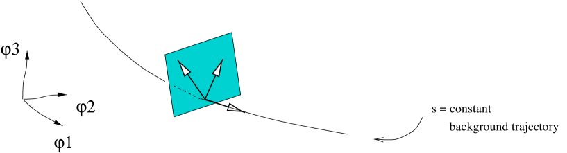
Figure 1: The new basis in N-dimensional field space. Here, $\sigma$ is a coordinate that varies along the background trajectory. It defines a basis vector ${\mathbf{\hat{e}}}_{\sigma}$ tangent to the curve. There are $N-1$ coordinates $s_{i}$ which are constant along the curve and define $N-1$ coordinate directions normal to it. The basis vectors along these directions ${\mathbf{\hat{e}}}_{s_{i}}$ are taken to be orthonormal and define the $N-1$ isocurvature perturbations.

Let us now focus for simplicity on a system with two fields and a diagonal metric

$$G_{AB}=\left(\begin{array}[]{cc}\alpha&0\\ 0&\beta\end{array}\right).$$ (78)

We take $s=0$ on the trajectory and we write (72) as

$$\Lambda^{1}{}_{\sigma}={U}(s)\frac{\varphi^{1^{\prime}}}{\sqrt{\alpha(\varphi^{1^{\prime}})^{2}+\beta(\varphi^{2^{\prime}})^{2}}}$$ (79)

$$\Lambda^{2}{}_{\sigma}={W}(s)\frac{\varphi^{2^{\prime}}}{\sqrt{\alpha(\varphi^{1^{\prime}})^{2}+\beta(\varphi^{2^{\prime}})^{2}}},$$ (80)

where we have parametrised the dependence on $s$ by the functions ${U}(s)$ and ${W}(s)$. On the trajectory ${U}(0)={W}(0)=1$. We take the unnormalised vector normal to the velocity to be

$$\tilde{\mathbf{\hat{e}}}_{s}={\mathbf{\hat{e}}}_{2}-({\mathbf{\hat{e}}}_{\sigma}\cdot{\mathbf{\hat{e}}}_{2}){\mathbf{\hat{e}}}_{\sigma}=\left(1-\beta(\Lambda^{1}{}_{\sigma})^{2}\right){\mathbf{\hat{e}}}_{2}-\beta\Lambda^{2}{}_{\sigma}\Lambda^{1}{}_{\sigma}{\mathbf{\hat{e}}}_{1}.$$ (81)

Therefore, the isocurvature basis vector is

$${\mathbf{\hat{e}}}_{s}=-\sqrt{\beta\over\alpha}\Lambda^{2}{}_{\sigma}{\mathbf{\hat{e}}}_{1}+\sqrt{\alpha\over\beta}\Lambda^{1}{}_{\sigma}{\mathbf{\hat{e}}}_{2},$$ (82)

from which we read off the transformation coefficients in the $s$ direction

$$\Lambda^{1}{}_{s}=-\sqrt{\beta\over\alpha}\Lambda^{2}{}_{\sigma},\,\,\,\Lambda^{2}{}_{s}=\sqrt{\alpha\over\beta}\Lambda^{1}{}_{\sigma}.$$ (83)

The metric in these new coordinates reads

$$G_{\sigma\sigma}=G_{ss}=\alpha\left(\Lambda^{1}{{}_{\sigma}}\right)^{2}+\beta\left(\Lambda^{2}{{}_{\sigma}}\right)^{2},$$ (84)

$$G_{s\sigma}=0,$$ (85)

which reduces to unit diagonal on the background trajectory, $s=0$, as expected.

In order to specify the new coordinate system completely, we need to know the functions $U$ and $W$ appearing in (79) and (80), or, equivalently, to be able to calculate a derivative of arbitrary order with respect to $s$ on the background trajectory, i.e at $s=0$. This can be achieved via (77) which in this case reads

$$\frac{dU}{ds}=-{W}\frac{1}{{\varphi^{1}}^{\prime}}{\partial\over\partial\tau}\left(\sqrt{\beta\over\alpha}{{\varphi^{2}}^{\prime}\over\sigma^{\prime}}\right)$$ (86)

and

$$\frac{dW}{ds}={U}\frac{1}{{\varphi^{2}}^{\prime}}{\partial\over\partial\tau}\left(\sqrt{\alpha\over\beta}{{\varphi^{1}}^{\prime}\over\sigma^{\prime}}\right).$$ (87)

With these, any derivative in the $\sigma,s$ coordinates can be calculated in terms of functions of $\tau$, known along the background trajectory.

We can now derive equations for the gravitational potential and the isocurvature perturbation at second order. The first term on the r.h.s of (60) is written in the $\sigma,\,s$ coordinates

$$\frac{8\pi}{m_{p}^{2}}a^{2}V_{C}\delta\varphi^{C}=\frac{8\pi}{m_{p}^{2}}a^{2}V_{,s}\delta{s}+\frac{8\pi}{m_{p}^{2}}a^{2}V_{,\sigma}\delta\sigma.$$ (88)

From (67)

$$a^{2}V_{,\sigma}\delta\sigma=\left(\frac{\sigma^{\prime\prime}}{\sigma^{\prime}}+2{\mathcal{H}}\right)\sigma^{\prime}\delta\sigma,$$ (89)

and from (51)

$$\sigma^{\prime}\delta\sigma=\frac{m_{p}^{2}}{4\pi}\left({\mathcal{H}}\psi+\psi^{\prime}\right)+\frac{m_{p}^{2}}{4\pi}\nabla^{-2}\left(\partial_{i}B_{i}\right).$$ (90)

So from (60) we can get an equation for the gravitational potential to second order

$$\psi^{\prime\prime}+2\left({\mathcal{H}}-\frac{\sigma^{\prime\prime}}{\sigma^{\prime}}\right)\psi^{\prime} + 2\left({\mathcal{H}}^{\prime}-{\mathcal{H}}\frac{\sigma^{\prime\prime}}{\sigma^{\prime}}\right)\psi=-\frac{8\pi}{m_{p}^{2}}\left(\sigma^{\prime}\right)^{2}\Gamma^{s}_{\sigma\sigma}\delta{s}$$ (91)

$$+ A-F^{\prime}-2\left({\sigma^{\prime\prime}\over\sigma^{\prime}}+3{\mathcal{H}}\right)F,$$

with

$$F\equiv\nabla^{-2}\partial_{i}B_{i}.$$ (92)

and we have used that on long wavelengths we have from (59)

$$F^{\prime}+2{\mathcal{H}}F={1\over 3}C.$$ (93)

We also need an equation for the entropy perturbation $\delta s$. We can get it by perturbing (38) expressed in the $\sigma,\,s$ coordinates:

$$\delta{}s^{\prime\prime} + 2{\mathcal{H}}\delta{}s^{\prime}-2\psi(\sigma^{\prime})^{2}\Gamma^{s}_{\sigma\sigma}+2\sigma^{\prime}\bigg{(}\delta\sigma^{\prime}\Gamma^{s}{}_{\sigma\sigma}+\delta{}s^{\prime}\Gamma^{s}{}_{s\sigma}\bigg{)}$$ (94)

$$+ (\sigma^{\prime})^{2}\bigg{(}\delta{}s\Gamma^{s}{}_{\sigma\sigma,s}+\delta\sigma\Gamma^{s}{}_{\sigma\sigma,\sigma}\bigg{)}+a^{2}G^{s\hat{F}}{}_{,\hat{C}}\delta\varphi^{\hat{C}}V_{,\hat{F}}+a^{2}V_{,s\hat{C}}\delta\varphi^{\hat{C}}=J^{s}.$$

Expressing $\delta\sigma$ and $\delta\sigma^{\prime}$ in terms of $\psi$ and $\psi^{\prime}$ we finally get

$$\delta{}s^{\prime\prime}+2{\mathcal{H}}\delta{}s^{\prime}+\left[a^{2}V_{ss}-6\left(\sigma^{\prime}\right)^{2}\Gamma^{s}_{\sigma\sigma}+\left(\sigma^{\prime}\right)^{2}\partial_{s}\Gamma^{s}_{\sigma\sigma}\right]=J^{s}.$$ (95)

The $J^{s}$ term appearing on the r.h.s of (95) is a second order source and it is calculated in the appendix. Equations (91) and (95) are generalisations to second order and a diagonal but otherwise arbitrary field metric of the equations for the evolution of long wavelength curvature and isocurvature perturbations given in [19]. The above procedure could of course be applied to an arbitrary number of fields and the most general metric.

A nice result proved in [19] is that when the background trajectory is straight in field space then isocurvature perturbations do not source the adiabatic one or, equivalently, the gravitational potential perturbation. This is true only if the metric is flat, $G_{AB}=\delta_{AB}$. If the field space has a nontrivial metric then the equivalent statement would be that this decoupling occurs if the background fields follow a geodesic in field space. By geodesics we mean the curves that the background fields would follow if there was no potential term in the lagrangian (36). We will now prove this for the two field case but the argument can be generalised in a straightforward manner. The geodesic equation in field space would read

$$\varphi^{A}{}^{\prime\prime}+2{\mathcal{H}}\varphi^{A}{}^{\prime}+\varphi^{B}{}^{\prime}\varphi^{C}{}^{\prime}\Gamma^{A}{}_{BC}=0.$$ (96)

In the $\sigma,\,s$ coordinates these equations read

$$\sigma^{\prime\prime}+2{\mathcal{H}}\sigma^{\prime} = 0$$

$$(\sigma^{\prime})^{2}\Gamma^{s}{}_{\sigma\sigma} = 0.$$ (97)

Hence, such trajectories correspond to $\Gamma^{s}{}_{\sigma\sigma}=0$ and from (91) we see that, indeed, the isocurvature perturbations do not source the metric perturbation . In contrast, for a “straight” trajectory $\Gamma^{s}{}_{\sigma\sigma}\neq 0$. Indeed

$$\Gamma^{s}{}_{\sigma\sigma} = \frac{1}{2}G^{s\hat{F}}\left(2G_{\hat{F}\sigma,\sigma}-G_{\sigma\sigma,\hat{F}}\right)$$ (98)

$$= \frac{1}{2}\left(2G_{s\sigma,\sigma}-G_{\sigma\sigma,s}\right)$$

$$= -\frac{1}{2}G_{\sigma\sigma,s}$$

where we have used that, by construction, $G_{\hat{A}\hat{B}}=\delta_{\hat{A}\hat{B}}$ along the trajectory. Now $G_{\sigma\sigma}=\Lambda^{A}{}_{\sigma}\Lambda^{B}{}_{\sigma}G_{AB}$ so

$$G_{\sigma\sigma,s} = 2\Lambda^{A}{}_{\sigma}\Lambda^{B}{}_{\sigma,s}G_{AB}+\Lambda^{A}{}_{\sigma}\Lambda^{B}{}_{\sigma}\Lambda^{C}{}_{s}G_{AB,C}$$ (99)

$$= 2G_{AB}\Lambda^{A}{}_{\sigma}\frac{1}{\sigma^{\prime}}\frac{\partial}{\partial\tau}\Lambda^{B}{}_{s}+\Lambda^{A}{}_{\sigma}\Lambda^{B}{}_{\sigma}\Lambda^{C}{}_{s}G_{AB,C}$$

from eq (77). In general the r.h.s of (99) will be different from zero. Hence $\Gamma^{s}{}_{\sigma\sigma}\neq 0$ and isocurvature perturbations can source the adiabatic one.

We conclude that nontrivial kinetic terms can lead to nontrivial couplings between the adiabatic and the isocurvature perturbations which may not be supressed on superhorizon scales, in contrast to what happens in models with flat field metrics . Such scalar Lagrangians appear in the effective actions of various candidate fundamental theories. Therefore it would be worth studying wether the interplay of isocurvature and adiabatic perturbations in such models has any interesting phenomenological consequences. Of course, non linear evolution will couple the two types of perturbations anyway.

3.3 Superhorizon Gauge Invariant Variables

Having found solutions to the perturbation equations at second order in a particular gauge, we can always construct gauge invariant quantities in terms of the new field coordinates $\sigma$ and $s_{i}$. At first order the gauge invariant curvature perurbation ${\mathcal{R}}$ is can be written as [19]

$${\mathcal{R}}_{(1)}=\left[\psi_{(1)}+\frac{{\mathcal{H}}}{\sigma^{\prime}}\delta\sigma_{(1)}\right]$$ (100)

Since $s^{\prime}=0$, $\delta{s_{i}}$ is gauge invariant at first order. At second order, according to eqn. (19)

$$\tilde{\delta}{s}=\delta{s}+2\xi_{(1)}^{0}\delta{s_{i}}_{(1)}^{\prime}$$ (101)

so a corresponding gauge invariant quantity is easily seen to be

$$\delta{s_{i}}^{(g.i)}=\delta{s_{i}}-2\frac{\delta\sigma_{(1)}}{\sigma^{\prime}}\delta{s_{i}}_{(1)}^{\prime}.$$ (102)

Similarly we can construct a gauge invariant curvature perturbation at second order similar to (28)

$${\mathcal{R}}_{(2)} = \left[\psi_{(2)}+\frac{{\mathcal{H}}}{\sigma^{\prime}}\delta\sigma_{(2)}\right]$$ (103)

$$+ \frac{\left[\psi_{(1)}^{\prime}+2{\mathcal{H}}\psi_{(1)}+\frac{{\mathcal{H}}}{\sigma^{\prime}}\delta_{(1)}\sigma^{\prime}\right]^{2}}{{\mathcal{H}}^{\prime}+2{\mathcal{H}}^{2}-{\mathcal{H}}\frac{\sigma^{\prime\prime}}{\sigma^{\prime}}}.$$

The variables (102) and (103) are second order gauge invariant variables (at least on superhorizon scales) which can be used to study isocurvature and adiabatic perurbations in the mild nonlinear regime.

4 Summary

We have touched upon the issue of studying second order perturbations in multifield inflationary models and defined gauge invariant variables - equations (102) and (103) - on supehorizon scales also to second order. The latter can be constructed given the solution to lowest non linear order in a given gauge. We have presented a more geometrical method for the splitting of isocurvature and adiabatic perturbations and applied it to a two field model with a diagonal but otherwise arbitrary metric. We showed that in this case naive “straight” trajectories do not lead to the decoupling of adiabatic from isocurvature perturbations. We identified the type of curves for which this happens. A perturbative approach by which one can study the nonlinear evolution of perturbations in such models to second order was suggested. The resulting equations have the same form as the first order linear ones but with new terms appearing on the right hand side. These new terms are quadratic in the first order perturbations and therefore they can be considered as known “sources” from the solution of the first order problem. Such a formalism can be used to calculate the amount of nongaussianity produced in such models by treating the perturbations as gaussian stochastic fields when they become superhorizon and then study their non linear evolution from that point. The resulting non gaussianity will be of the $\chi^{2}$ type since we are considering quadratic products of gaussian fields. We have implicitly assumed a smoothing on scales larger than the horizon and dropped second order spatial gradients. Although straightforward to calculate, the resulting source terms, in principle known, are quite complicated. We will return to the issue of calculating non linear evolution in multifield inflationary models with a different approach in a future publication [12].

Acknowledgements: Many thanks to Carsten van de Bruck and Christopher Gordon for useful discussions and comments, Marco Bruni for bringing to my attention other works related to second order perturbation theory, and especially Paul Shellard for discussions and generous support.

Appendix A Second order sources

In this appendix we give formulae nessecary for the calculation of the terms A, C, F, $J^{s}$ defined in the text. These are the terms containing products of first order perturbations.

We write the metric as

$$g_{\mu\nu}=g_{\mu\nu}^{B}+h_{\mu\nu}.$$ (104)

where $h_{0i}=0$. Indices will be raised and lowered with the background metric. Then the perturbation of the contravariant metric tensor will be

$$g^{\mu\nu}=g^{(B)\mu\nu}-h^{\mu\nu}+h^{\mu}{}_{\alpha}h^{\alpha\nu}$$ (105)

and in particular

$$g^{00} = \frac{1}{a^{2}}-\frac{1}{a^{4}}h_{00}+\frac{1}{a^{6}}h_{00}h_{00}$$ (106)

$$g^{0i} = 0$$ (107)

$$g^{ij} = -\frac{\delta_{ij}}{a^{2}}-\frac{1}{a^{4}}h_{ij}-\frac{1}{a^{6}}h_{ik}h_{kj}.$$ (108)

The perturbation of the metric determinant is

$$\sqrt{-g}=a^{4}\left(1+\frac{1}{2}h+\frac{1}{8}h^{2}-\frac{1}{4}h^{\alpha}{}_{\beta}h^{\beta}{}_{\alpha}\right).$$ (109)

The perturbation of the Riemann tensor to first and second order can be found to be ([23] p:965)

$$R^{(1)}_{\mu\nu}=\frac{1}{2}\left(-h_{|\mu\nu}-h_{\mu\nu|\alpha}{}^{\alpha}+h_{\alpha\mu|\nu}{}^{\alpha}+h_{\alpha\nu|\mu}{}^{\alpha}\right)$$ (110)

and

$$R^{(2)}_{\mu\nu} = \frac{1}{2}\bigg{[}\frac{1}{2}h_{\alpha\beta{|}\mu}h^{\alpha\beta}{}_{|\nu}+h^{\alpha\beta}\left(h_{\alpha\beta|\mu\nu}+h_{\mu\nu|\alpha\beta}-h_{\alpha\mu|\nu\beta}-h_{\alpha\nu|\mu\beta}\right)$$ (111)

$$+ h_{\nu}{}^{\alpha|\beta}\left(h_{\alpha\mu|\beta}-h_{\beta\mu|\alpha}\right)-\left(h^{\alpha\beta}{}_{|\beta}-\frac{1}{2}h^{|\alpha}\right)\left(h_{\alpha\mu|\nu}+h_{\alpha\nu|\mu}-h_{\mu\nu|\alpha}\right)\bigg{]}.$$

where a vertical bar denotes a covariant derivative w.r.t. the background. Then

$$R^{(1)\mu}{}_{\nu}=g^{(B)\mu\alpha}R^{(1)}{}_{\alpha\nu}-h^{\mu\alpha}R^{(B)}{}_{\alpha\nu}$$ (112)

and

$$R^{(2)\mu}{}_{\nu}=g^{(B)\mu\alpha}R^{(2)}_{\alpha\nu}-h^{\mu\alpha}R_{(1)\alpha\nu}+h^{\mu}{}_{\lambda}h^{\lambda\alpha}R^{(B)}_{\alpha\nu}.$$ (113)

Using the following perturbed metric tensor (longitudinal gauge)

$$h_{00}=2a^{2}\psi$$ (114)

$$h_{ij}=2a^{2}\psi\delta_{ij}-2a^{2}E_{ij}$$ (115)

$$h=-4\psi$$ (116)

we get, after a rather tedious calculation

$$R^{(2)0}{}_{0}=\frac{2}{a^{2}}\bigg{[}-6{\mathcal{H}}\psi^{\prime}\psi-6\left({\mathcal{H}}^{\prime}+2{\mathcal{H}}^{2}\right)\psi^{2}-E_{kl}\left({\mathcal{H}}{E_{kl}^{\prime}}+2{\mathcal{H}}^{2}E_{kl}\right)+\frac{1}{2}E^{\prime}_{kl}E^{\prime}_{kl}\bigg{]},$$ (117)

$$R^{(2)0}{}_{i}=\frac{2}{a^{2}}\bigg{[}\partial_{i}\psi\left(\psi^{\prime}-4{\mathcal{H}}\psi\right)+2E_{kl}\left(\partial_{i}E_{kl}^{\prime}-\partial_{l}E_{ki}^{\prime}\right)+E_{kl}^{\prime}\partial_{i}E_{kl}+2E_{il}\partial_{l}\psi^{\prime}-2\partial_{l}\psi{}E_{il}^{\prime}\bigg{]},$$ (118)

$$R^{(2)i}{}_{j} = -\frac{4}{a^{2}}\bigg{[}\psi\left({\mathcal{H}}\psi^{\prime}-({\mathcal{H}}^{\prime}+2{\mathcal{H}}^{2})\psi\right)\delta_{ij}+\frac{1}{2}(\psi^{\prime})^{2}\delta_{ij}$$ (119)

$$+ \frac{1}{2}{E}_{ij}\left(\psi^{\prime\prime}+2{\mathcal{H}}\psi^{\prime}+2(4{\mathcal{H}}^{\prime}+9{\mathcal{H}}^{2})\psi\right)$$

$$- \frac{1}{2}{\mathcal{H}}{}E^{\prime}_{ik}E_{kj}-\frac{1}{2}{\mathcal{H}}{}E^{\prime}_{kl}E_{kl}\delta_{ij}-\frac{1}{4}({\mathcal{H}}^{\prime}+2{\mathcal{H}}^{2})E_{ik}E_{kj}\bigg{]}.$$

The Einstein tensor will be

$$G^{(2)0}{}_{0}=\frac{1}{2}\left(R^{(2)0}{}_{0}-R^{(2)l}{}_{l}\right)$$ (120)

$$G^{(2)0}{}_{i}=R^{(2)0}{}_{i}$$ (121)

$$G^{(2)i}{}_{j}=R^{(2)i}{}_{j}-\frac{1}{2}\delta^{i}{}_{j}\left(R^{(2)0}{}_{0}-R^{(2)i}{}_{i}\right),$$ (122)

so we find

$$G^{(2)0}{}_{0} = \frac{1}{a^{2}}\bigg{[}-6\psi\left(({\mathcal{H}}^{\prime}+2{\mathcal{H}}^{2})\psi\right)+3(\psi^{\prime})^{2}$$ (123)

$$- E_{kl}\left(5{\mathcal{H}}{}E_{kl}^{\prime}+(\frac{9}{2}{\mathcal{H}}^{2}-{\mathcal{H}}^{\prime})E_{kl}\right)+\frac{1}{2}E_{kl}^{\prime}E_{kl}^{\prime}\bigg{]},$$

$$G^{(2)0}{}_{i} = \frac{2}{a^{2}}\bigg{[}\partial_{i}\psi\left(\psi^{\prime}-4{\mathcal{H}}\psi\right)+2E_{kl}\left(\partial_{i}E_{kl}^{\prime}-\partial_{l}E_{ki}^{\prime}\right)$$ (124)

$$+ E_{kl}^{\prime}\partial_{i}E_{kl}+2E_{il}\partial_{l}\psi^{\prime}-2\partial_{l}\psi{}E_{il}^{\prime}\bigg{]},$$

$$G^{(2)i}{}_{j} = \frac{3}{a^{2}}\bigg{[}2\psi\left(4{\mathcal{H}}\psi^{\prime}+2({\mathcal{H}}^{\prime}+2{\mathcal{H}}^{2})\psi\right)\delta_{ij}+(\psi^{\prime})^{2}\delta_{ij}$$ (125)

$$+ 2{\mathcal{H}}{}E_{ki}^{\prime}E_{kj}-{\mathcal{H}}{}E_{kl}^{\prime}E_{kl}\delta_{ij}+({\mathcal{H}}^{\prime}+2{\mathcal{H}}^{2})E_{ki}E_{kj}$$

$$- \frac{1}{2}({\mathcal{H}}^{2}-2{\mathcal{H}}^{\prime})E_{kl}E_{kl}\delta_{ij}-\frac{1}{2}E^{\prime}_{kl}E^{\prime}_{kl}\delta_{ij}$$

$$- 2E_{ij}\left(\psi^{\prime\prime}+2{\mathcal{H}}\psi^{\prime}+2(4{\mathcal{H}}^{\prime}+9{\mathcal{H}}^{2})\psi\right)\bigg{]}.$$

For the energy momentum tensor

$$T_{\mu\nu}=G_{AB}\partial_{\mu}\varphi^{A}\partial_{\nu}\varphi^{B}-g_{\mu\nu}\left[\frac{1}{2}G_{AB}\partial_{\lambda}\varphi^{A}\partial^{\lambda}\varphi^{B}-V(\varphi)\right].$$ (126)

the second order perturbation for two fields is given by

$$T^{(2)0}{}_{0} = \frac{1}{a^{2}}\bigg{[}\left(\delta\sigma^{\prime}\right)^{2}-2\sigma^{\prime}\left(\Gamma^{s}_{\sigma\sigma}\right)^{\prime}\delta s\delta\sigma-\left(\sigma^{\prime}\right)^{2}\partial_{s}\Gamma^{s}_{\sigma\sigma}\delta s^{2}$$ (127)

$$+ 2\psi^{2}\left(\sigma^{\prime}\right)^{2}+2\left(\sigma^{\prime}\right)^{2}\Gamma^{s}_{\sigma\sigma}\psi\delta s-2\Gamma^{s}_{\sigma\sigma}\sigma^{\prime}\delta s\delta\sigma^{\prime}-2\sigma^{\prime}\psi\delta\sigma^{\prime}\bigg{]}$$

$$+ V_{ss}\delta s^{2}+2V_{s\sigma}\delta s\delta\sigma+V_{\sigma\sigma}\delta\sigma^{2}$$

$$T^{(2)0}{}_{i}=\frac{1}{a^{2}}\left[\delta{}s^{\prime}\partial_{i}\delta{}s+\left(\delta\sigma^{\prime}-2\sigma^{\prime}\Gamma^{s}_{\sigma\sigma}\delta{}s-2\psi\sigma^{\prime}\right)\partial_{i}\delta\sigma\right],$$ (128)

$$T^{(2)i}{}_{j} = -\delta^{i}_{j}\frac{1}{a^{2}}\bigg{[}\left(\delta\sigma^{\prime}\right)^{2}-2\sigma^{\prime}\left(\Gamma^{s}_{\sigma\sigma}\right)^{\prime}\delta s\delta\sigma-\left(\sigma^{\prime}\right)^{2}\partial_{s}\Gamma^{s}_{\sigma\sigma}\delta s^{2}$$ (129)

$$+ 2\psi^{2}\left(\sigma^{\prime}\right)^{2}+2\left(\sigma^{\prime}\right)^{2}\Gamma^{s}_{\sigma\sigma}\psi\delta s-2\Gamma^{s}_{\sigma\sigma}\sigma^{\prime}\delta s\delta\sigma^{\prime}-2\sigma^{\prime}\psi\delta\sigma^{\prime}\bigg{]}$$

$$+ \delta^{i}_{j}\left[V_{ss}\delta s^{2}+2V_{s\sigma}\delta s\delta\sigma+V_{\sigma\sigma}\delta\sigma^{2}\right]$$

where we have obviously dropped second order spatial derivatives. We also need to compute the quadratic part of the wave equation for the system of scalar fields

$$\frac{1}{\sqrt{-g}}\partial_{\mu}\left(\sqrt{-g}g^{\mu\nu}\partial_{\nu}\varphi^{A}\right)+g^{\mu\nu}\partial_{\mu}\varphi^{B}\partial_{\nu}\varphi^{C}\Gamma^{A}_{BC}+G^{AF}V_{,F}=0.$$ (130)

Up to second order spatial gradients we get

$$J^{s} = -4{d\over d\tau}\left(a^{2}\psi\delta s^{\prime}\right)+4a^{2}\left(\sigma^{\prime}\right)^{2}\Gamma^{s}_{\sigma\sigma}\left(\psi^{2}+\Gamma^{s}_{\sigma\sigma}\psi\delta s\right)$$ (131)

$$+ a^{2}\sigma^{\prime}\left(\Gamma^{s}_{\sigma\sigma}\right)^{\prime}\left[-3\psi\delta\sigma+2{\delta\sigma\delta\sigma^{\prime}\over\sigma^{\prime}}+2{\delta\sigma\delta s^{\prime}\over\sigma^{\prime}}+4\Gamma^{s}_{\sigma\sigma}\delta s\delta\sigma\right]$$

$$+ a^{2}\partial_{s}\Gamma^{s}_{\sigma\sigma}\left[-2\delta s^{2}-3\left(\sigma^{\prime}\right)^{2}\psi\delta s+2{\sigma^{\prime}\delta s\delta\sigma^{\prime}}+2{\sigma^{\prime}\delta s\delta s^{\prime}}\right]$$

$$+ a^{2}\left(\sigma^{\prime}\right)^{2}\delta\sigma\left[{1\over\sigma^{\prime}}{d\over d\tau}\left({1\over\sigma^{\prime}}\left(\Gamma^{s}_{\sigma\sigma}\right)^{\prime}\right)+{1\over\sigma^{\prime}}{d\over d\tau}\left(\partial_{s}\Gamma^{s}_{\sigma\sigma}\right)\right]$$

$$- 2a^{4}\psi\left(V_{ss}\delta s+V_{s\sigma}\delta\sigma\right)+a^{4}\left(V_{sss}\delta{}s^{2}+2V_{ss\sigma}\delta{}s\delta\sigma+V_{s\sigma\sigma}\delta\sigma^{2}\right)\bigg{]}$$

$$+ a^{2}\left(\sigma^{\prime}\right)^{2}\Gamma^{s}_{\sigma\sigma}E_{ij}E_{ij}.$$

With these formulae we can compute all the second order terms defined in the text.

Appendix B Isocurvature-adiabatic split with three fields

In this appendix we present the isocurvature-adiabatic split for three fields $\varphi^{1},\,\varphi^{2},\,\varphi^{3}$ with an arbitrary metric $G_{AB}$. This should illustrate the general case. Now we will have two isocurvature directions. Take the set $\{{\mathbf{\hat{e}}}_{\sigma},\,{\mathbf{\hat{e}}}_{2},\,{\mathbf{\hat{e}}}_{3}\}$ as the starting point for constructing the orthonormal vectors. Form ${\mathbf{\hat{e}}}_{s_{2}}$ which lies in the plane spanned by ${\mathbf{\hat{e}}}_{\sigma}$ and ${\mathbf{\hat{e}}}_{2}$. First form the unnormalised

$$\tilde{\mathbf{\hat{e}}}_{s_{2}}={\mathbf{\hat{e}}}_{2}-({\mathbf{\hat{e}}}_{2}\cdot{\mathbf{\hat{e}}}_{\sigma}){\mathbf{\hat{e}}}_{\sigma}$$ (132)

One finds

$$\tilde{\mathbf{\hat{e}}}_{s_{2}}=\tilde{\Lambda}^{A}{}_{s_{2}}{\mathbf{\hat{e}}}_{A}$$ (133)

with

$$\tilde{\Lambda}^{2}{}_{s_{2}} = 1-\Lambda_{2\sigma}\Lambda^{2}{}_{\sigma}=\Lambda_{1\sigma}\Lambda^{1}{}_{\sigma}+\Lambda_{3\sigma}\Lambda^{3}{}_{\sigma}$$

$$\tilde{\Lambda}^{1}{}_{s_{2}} = -\Lambda_{2\sigma}\Lambda^{1}{}_{\sigma}$$

$$\tilde{\Lambda}^{3}{}_{s_{2}} = -\Lambda_{2\sigma}\Lambda^{3}{}_{\sigma},$$ (134)

where

$$\Lambda_{A\sigma}\equiv{}G_{AB}\Lambda^{B}{}_{\sigma}.$$ (135)

Then

$${\mathbf{\hat{e}}}_{s_{2}}=\frac{\tilde{\Lambda}^{A}{}_{s_{2}}}{\sqrt{\tilde{\Lambda}^{B}{}_{s_{2}}\tilde{\Lambda}_{Bs_{2}}}}{\mathbf{\hat{e}}}_{A}.$$ (136)

So, we have

$$\Lambda^{A}{}_{s_{2}}=\frac{\tilde{\Lambda}^{A}{}_{s_{2}}}{\sqrt{\tilde{\Lambda}^{B}{}_{s_{2}}\tilde{\Lambda}_{Bs_{2}}}}.$$ (137)

Repeating the procedure we form

$$\tilde{\mathbf{\hat{e}}}_{s_{3}}={\mathbf{\hat{e}}}_{3}-({\mathbf{\hat{e}}}_{3}\cdot{\mathbf{\hat{e}}}_{\sigma}){\mathbf{\hat{e}}}_{\sigma}-({\mathbf{\hat{e}}}_{3}\cdot{\mathbf{\hat{e}}}_{s_{2}}){\mathbf{\hat{e}}}_{s_{2}}$$ (138)

to get

$$\tilde{\Lambda}^{1}{}_{s_{3}} = -\Lambda_{3\sigma}\Lambda^{1}{}_{\sigma}-\Lambda_{3s_{2}}\Lambda^{1}{}_{s_{2}}$$

$$\tilde{\Lambda}^{2}{}_{s_{3}} = -\Lambda_{3\sigma}\Lambda^{2}{}_{\sigma}-\Lambda_{3s_{2}}\Lambda^{2}{}_{s_{2}}$$

$$\tilde{\Lambda}^{3}{}_{s_{3}} = 1-\Lambda_{3\sigma}\Lambda^{3}{}_{\sigma}-\Lambda_{3s_{2}}\Lambda^{3}{}_{s_{2}}.$$ (139)

So we have

$$\Lambda^{A}{}_{s_{3}}=\frac{\tilde{\Lambda}^{A}{}_{s_{3}}}{\sqrt{\tilde{\Lambda}^{B}{}_{s_{3}}\tilde{\Lambda}_{Bs_{3}}}}.$$ (140)

As before, we demand for the ${\mathbf{\hat{e}}}_{s_{i}}$‘s

$$\left[{{\mathbf{\hat{e}}}_{s_{i}}},\,{\mathbf{\hat{e}}}_{\sigma}\right]=0$$ (141)

from which we get by acting on $\varphi^{A}$

$$\frac{1}{\sigma^{\prime}}\frac{\partial}{\partial\tau}\Lambda^{A}{}_{s_{2}}=\frac{\partial}{\partial{}s_{2}}\Lambda^{A}{}_{\sigma}$$ (142)

$$\frac{1}{\sigma^{\prime}}\frac{\partial}{\partial\tau}\Lambda^{A}{}_{s_{3}}=\frac{\partial}{\partial{}s_{3}}\Lambda^{A}{}_{\sigma}.$$ (143)

Knowing the $\Lambda$ coefficients we can calculate the metric $G_{\hat{A}\hat{B}}$ in the new basis, where the index $\hat{A}$ runs over $\{\sigma,\,s_{1},\,s_{2}\}$. Using equations (142) and (143) we can then calculate any partial derivative of $\Lambda^{A}{}_{\sigma}$ in terms of time derivatives along the background trajectory. Hence we can calculate the connection and perturbations of arbitrary order in the new $\{{\mathbf{\hat{e}}}_{\sigma},\,{\mathbf{\hat{e}}}_{s_{1}},\,{\mathbf{\hat{e}}}_{s_{2}}\}$ basis.

References

- [1] D.Wands, K.A. Malik, D.H. Lyth, A.R. Liddle, Phys.Rev.D62, 043527 (2000)
- [2] A. Gangui, F. Lucchin, S. Matarrese, S. Mollerach, Astrophys.J. 430:447-457, 1994, astro-ph/9312033,
- [3] D.S. Salopek, J.R. Bond, Phys.Rev.D43:1005-1031,1991, ibid. Phys.Rev.D42:3936-3962,1990,
- [4] J. Maldacena, JHEP 0305:013, 2003, astro-ph/0210603
- [5] V. Acquaviva, N Bartolo, S. Matarrese, A. Riotto, Nucl.PhysB667, 119-148, 2003, astro-ph/0209156
- [6] A. Gangui, J Martin and M. Sakellariadou, Phys.Rev.D66, 083502 (2002)
- [7] E. Komatsu, Ph.D. Thesis, astro-ph/0206039
- [8] I. Yi, E.T. Vishniac, 1993ApJS, vol.86, no.2, p.333-364
-
[9]
G.L. Comer et. al, Phys.Rev.D 49, 2759(1994),
N. Deruelle & D. Langlois, Phys.Rev.D 52, 2007(1995) and references therein,
J. Parry et. al. Phys.Rev.D 49, 2872(1994)
I.M. Khalatnikov et. al, Class.Quant.Grav. 19(2002) 3845 - [10] F. Bernardeau and J. Uzan, Phys.Rev.D66, 103506 (2002); ibid. Phys.Rev.D67, 121301(R) (2003)
- [11] E. Komatsu et. al., Astrophys.J.Suppl.148:119-134,2003
- [12] G. Rigopoulos and E.P.S. Shellard, in preparation.
- [13] E. Lifshitz, Zh.Eksp.Teor.Fiz 16(1946) 587, translated in English in J.Phys.(USSR) 10(1946) 116,
- [14] V.F. Mukhanov, H.A. Feldman and R.H. Brandenberger, PHYSICS REPORTS 215, (1992)203-333
- [15] J.M. Stewart, Class. Quant. Grav. 7 (1990) 1169-1180
- [16] V. Lukash, JETP 52, 807 (1980),
- [17] M. Bruni, S. Matarrese, S. Mollerach, S. Sonego, Class. Quant. Grav. 14(1997) 2585-2606
- [18] M. Bruni, S. Sonego, Class. Quant. Grav. 16(1999) L29-L36
- [19] C. Gordon, D. Wands, B.A. Bassett, R. Maartens, Phys.Rev. D 63 023506 (2001), astro-ph/0009131
- [20] S. Groot Nibbelink and B.J.W. van Tent, Class.Quant.Grav. 19(2002) 613-640
- [21] K.A. Malik and D.Wands, Phys.Rev.D59, 123501 (1999)
- [22] F. DiMarco, F. Finelli, R. Brandenberger, astro-ph/0211276
- [23] Misner C W, Thorne K S and Wheeler J A, 1973 “Gravitation” (Freeman: New York).