Stability of the viscously spreading ring

We study analytically and numerically the stability of the pressure-less, viscously spreading accretion ring. We show that the ring is unstable to small non-axisymmetric perturbations. To perform the perturbation analysis of the ring we use a stretching transformation of the time coordinate. We find that to 1st order, one-armed spiral structures, and to 2nd order additionally two-armed spiral features may appear. Furthermore, we identify a dispersion relation determining the instability of the ring. The theoretical results are confirmed in several simulations, using two different numerical methods. These computations prove independently the existence of a secular spiral instability driven by viscosity, which evolves into persisting leading and trailing spiral waves. Our results settle the question whether the spiral structures found in earlier simulations of the spreading ring are numerical artifacts or genuine instabilities.

1 Introduction

In the theory of accretion discs, the idealised problem of a viscously spreading, pressure-less ring orbiting a central point mass on Keplerian orbits is often used to exemplify the main features of an evolving thin accretion disc, i.e. the inward transport of mass and outward transport of angular momentum (Pringle, 1981; Frank et al., 2002). With the approximation of a small kinematic viscosity $\nu$ that is independent of the surface density, an analytic solution exists for this problem, stated originally by Lüst (1952) and later by Lynden-Bell & Pringle (1974).

This axisymmetric analytic solution of the viscous dust ring is frequently used as test problem for numerical methods developed to simulate accretion discs. The tested algorithms cover particle methods like smoothed particle hydrodynamics (SPH) (e.g. Flebbe et al., 1994; Speith & Riffert, 1999) as well as grid-based codes like RH2D (e.g. Kley, 1999).

However, numerical simulations of the evolving ring often show the appearance of additional structures in the disc. In the majority of cases, these structures consist of non-axisymmetric one-armed spirals, but eventually also narrow concentric rings appear. Since their first discovery, it is controversially debated whether these structures are numerical artifacts or mathematical instabilities. While Maddison et al. (1996) show that for the axisymmetric case the concentric rings found in SPH simulations are numerical artifacts of the method, we demonstrate in this paper that the non-axisymmetric spiral structures result from a genuine physical instability of the problem.

Recently, Ogilvie (2001) analysed radially extended accretion discs in a work presenting a general model of eccentric accretion discs, of which the viscous ring is a simple special case. However, because his main objective was much wider, he did not elaborate on the stability properties of the ring.

The remainder of the paper is organised as follows. In the next section, we first summarise the basic hydrodynamic equations used for our analysis of the evolving disc, and present for reference the analytic solution of the viscously spreading dust ring.

In Sect. 3 we use a special perturbation technique, the time-stretching approach, which allows to obtain solutions of the spreading ring at different orders of a small expansion parameter. We derive a linear evolution equation for an eccentricity function $E$. It is shown that to 2nd order, the general solution allows the development of one-armed as well as two-armed spiral features.

In Sect. 4 we perform a local stability analysis of the final equation for $E$ and deduce a dispersion relation which indicates an instability for some viscosity laws. These results are compared with numerical simulations we present in Sect. 5 using two different numerical methods, one grid-based and the other particle based. We find in general very good agreement of both numerical methods with the predictions of the local analysis. Thus, the simulations confirm the existence of a physical instability in the viscously evolving ring problem. Finally, in 6 we give our conclusions.

2 The equations

In accretion physics one assumes that the evolution of the disc can be modelled by the hydrodynamic equations. In the present case, we envisage a thin accretion disc, i.e. the vertical thickness of the disc is very small in comparison to the radial extend. Therefore, the evolution of the surface density $\Sigma$ of the disc can be modelled by the vertically averaged hydrodynamic equations which reduces the problem to two dimensions and formally corresponds to the 2D-version of the hydrodynamic equations.

2.1 Basic hydrodynamic equations

Because of the axisymmetry of the ring solution, it is convenient to work in polar coordinates $(R,\varphi)$. In the presence of a central gravitational field originating by the mass $M_{\mathrm{c}}$, the set of the basic hydrodynamic equations consists of the continuity equation

$$\frac{\partial\Sigma}{\partial t}+\frac{1}{R}\frac{\partial(R\Sigma v_{R})}{\partial R}+\frac{1}{R}\frac{\partial(\Sigma v_{\varphi})}{\partial\varphi}=0\quad,$$ (1)

the radial component of the Navier Stokes equation

$$\Sigma\left(\frac{\partial v_{R}}{\partial t}+v_{R}\frac{\partial v_{R}}{\partial R}+\frac{v_{\varphi}}{R}\frac{\partial v_{R}}{\partial\varphi}-\frac{v_{\varphi}^{2}}{R}\right)=-\frac{\partial p_{s}}{\partial R}-\Sigma\frac{GM_{\mathrm{c}}}{R^{2}}$$ (2)

$${}+\frac{1}{R}\frac{\partial(R\nu_{s}\Sigma\sigma_{RR})}{\partial R}+\frac{1}{R}\frac{\partial(\nu_{s}\Sigma\sigma_{R\varphi})}{\partial\varphi}-\frac{\nu_{s}\Sigma}{R}\sigma_{\varphi\varphi}\quad,$$

and the azimuthal component of the Navier Stokes equation

$$\Sigma\left(\frac{\partial v_{\varphi}}{\partial t}+v_{R}\frac{\partial v_{\varphi}}{\partial R}+\frac{v_{\varphi}}{R}\frac{\partial v_{\varphi}}{\partial\varphi}+\frac{v_{R}v_{\varphi}}{R}\right)=-\frac{1}{R}\frac{\partial p_{s}}{\partial\varphi}$$ (3)

$${}+\frac{1}{R}\frac{\partial(R\nu_{s}\Sigma\sigma_{R\varphi})}{\partial R}+\frac{1}{R}\frac{\partial(\nu_{s}\Sigma\sigma_{\varphi\varphi})}{\partial\varphi}+\frac{\nu_{s}\Sigma}{R}\sigma_{R\varphi}\quad.$$

Here $v_{R}$ and $v_{\varphi}$ denote the radial and azimuthal velocity, $p_{s}$ is the vertically averaged pressure, and $G$ is the gravitational constant. Assuming that the bulk viscosity is vanishing, the viscous shear tensor $\sigma$ has the form

$$\sigma_{RR} = \frac{4}{3}\frac{\partial v_{R}}{\partial R}-\frac{2}{3}\frac{v_{R}}{R}-\frac{2}{3}\frac{1}{R}\frac{\partial v_{\varphi}}{\partial\varphi}\quad,$$ (4)

$$\sigma_{R\varphi} = \sigma_{\varphi R}\;=\;\frac{\partial v_{\varphi}}{\partial R}-\frac{v_{\varphi}}{R}+\frac{1}{R}\frac{\partial v_{R}}{\partial\varphi}\quad,$$ (5)

$$\sigma_{\varphi\varphi} = -\frac{2}{3}\frac{\partial v_{R}}{\partial R}+\frac{4}{3}\frac{v_{R}}{R}+\frac{4}{3}\frac{1}{R}\frac{\partial v_{\varphi}}{\partial\varphi}\quad,$$ (6)

and $\nu_{s}$ is the vertically averaged kinematic viscosity.

As we only consider cold (pressure-less) discs, we neglect the pressure $p_{s}$ throughout the rest of this paper.

2.2 Analytic solution of the viscous ring

For the time evolution of the viscously spreading ring, we assume $\nu_{s}=\mathrm{const.}$ Then, with initial condition

$$\Sigma_{\mathrm{init}}(R)=\frac{M}{2\pi R_{0}}\delta(R-R_{0})$$ (7)

at $t=0$ with total ring mass $M$, the surface density of the ring evolves according to

$$\Sigma_{\mathrm{ring}}(\tau^{*},x)=\frac{M}{\pi R_{0}^{2}}\frac{1}{\tau^{*}x^{1/4}}\;I_{\frac{1}{4}}\!\!\left(\frac{2x}{\tau^{*}}\right)\,\exp\!\left(-\frac{1+x^{2}}{\tau^{*}}\right)$$ (8)

(e.g. Lynden-Bell & Pringle, 1974), where $x=R/R_{0}$, $\tau^{*}=12\nu_{s}t/R_{0}^{2}$, and $I_{\frac{1}{4}}$ is the modified Bessel function to the order of 1/4.

The azimuthal velocity of the ring is equal to Keplerian velocity,

$$v_{\mathrm{Kepler}}=\sqrt{\frac{GM_{\mathrm{c}}}{R}}=\Omega R\quad,$$ (9)

where we have defined the angular velocity

$$\Omega(R)=\sqrt{\frac{GM_{\mathrm{c}}}{R^{3}}}\quad.$$ (10)

The radial velocity of the ring obeys the relation

$$v_{\mathrm{spreading}}=-\frac{3}{\Sigma_{\mathrm{ring}}\sqrt{R}}\frac{\partial}{\partial R}\left[\nu_{s}\Sigma_{\mathrm{ring}}\sqrt{R}\right]\quad.$$ (11)

It is important to realize, that solution (8) fulfils the hydrodynamic equations given in 2.1 only by approximation, assuming the kinematic viscosity $\nu_{s}$ being small compared to the specific angular momentum $\Omega R^{2}$.

3 Perturbation analysis

To study the stability properties of the ring solution (8), we perform a perturbation analysis of the hydrodynamic equations (1), (2) and (3).

3.1 Stretching transformation

According to the idealised problem, we assume that the averaged kinematic viscosity $\nu_{s}$ is very small and depends only on $R$. To take this into account, we replace

$$\nu_{s}=\nu_{s}(R)=\epsilon\,\nu(R)\quad\mbox{where}\quad\epsilon=\mathrm{const.}\ll 1\quad.$$ (12)

Then, two different timescales can be distinguished, the viscous timescale $t_{\mathrm{visc}}\sim R^{2}/\nu_{s}$ which determines the radial spreading of the ring, and the dynamic timescale $t_{\mathrm{dyn}}\sim R/v_{\varphi}=\sqrt{R^{3}/GM_{\mathrm{c}}}$ describing the azimuthal motion of the gas in the disc. Because of (12), the dynamic timescale is much shorter than the viscous timescale, $t_{\mathrm{dyn}}/t_{\mathrm{visc}}\sim\nu_{s}/\sqrt{GM_{\mathrm{c}}R}=\epsilon\,\nu/(\Omega R^{2})\ll 1$. Therefore, in addition to the dynamic time $t$ we define a viscous time

$$\tau=\epsilon\,t\quad.$$ (13)

In principle, the ring may evolve on the dynamic timescale as well as on the viscous timescale. Thus we assume for the time dependencies of all hydrodynamic quantities

$$\Sigma(t)=\hat{\Sigma}(t,\tau)\,,\;v_{R}(t)=\hat{v}_{R}(t,\tau)\,,\;v_{\varphi}(t)=\hat{v}_{\varphi}(t,\tau)\;.$$ (14)

This leads to a stretching transformation for the time derivatives,

$$\frac{\partial f(t)}{\partial t}=\frac{\partial\hat{f}(t,\tau)}{\partial t}+\epsilon\,\frac{\partial\hat{f}(t,\tau)}{\partial\tau}\quad,$$ (15)

where $f$ symbolises any of the hydrodynamic quantities.

3.2 Approach

To generalise the approach, we do not restrict the stability analysis to a perturbation of the ring solution (8) but we start with less determined unperturbed functions. The initial condition of the problem shall consist of an arbitrary axisymmetric surface density distribution $\Sigma_{\rm init}(R)$ rotating around a central mass $M_{\mathrm{c}}$. Because self gravity of the disc can be neglected, the initial azimuthal velocity shall be equal to the Keplerian velocity (9), $v_{\varphi}^{\mathrm{init}}=v_{\mathrm{Kepler}}$. Then, the following approach is made for the expansion

$$\Sigma(t,R,\varphi) = \hat{\Sigma}_{0}(t,\tau,R)+\epsilon\,\hat{\Sigma}_{1}(t,\tau,R,\varphi)$$ (16)

$${}+\epsilon^{2}\,\hat{\Sigma}_{2}(t,\tau,R,\varphi)+{\cal O}(\epsilon^{3})\quad,$$

$$v_{R}(t,R,\varphi) = \hat{v}_{R0}(t,\tau,R)+\epsilon\,\hat{v}_{R1}(t,\tau,R,\varphi)$$ (17)

$${}+\epsilon^{2}\,\hat{v}_{R2}(t,\tau,R,\varphi)+{\cal O}(\epsilon^{3})\quad,$$

$$v_{\varphi}(t,R,\varphi) = \hat{v}_{\varphi 0}(\tau,R)+\epsilon\,\hat{v}_{\varphi 1}(t,\tau,R,\varphi)$$ (18)

$${}+\epsilon^{2}\,\hat{v}_{\varphi 2}(t,\tau,R,\varphi)+{\cal O}(\epsilon^{3})\quad.$$

Here it is assumed that the 0th order quantities are axisymmetric and do not depend on the azimuthal angle $\varphi$, and that the 0th order azimuthal velocity evolves only very slowly and is independent of the dynamical time $t$ (both assumptions are justified by the initial conditions).

The approaches (16), (17) and (18) are inserted in (1), (2) and (3) considering the stretching transformation (15) and (12), and the terms of the resulting equations are ordered according to powers of $\epsilon$.

There are three main differences of the present approach compared to previous analyses like those by Ogilvie (2001). The kinematic viscosity is assumed to be a function of radius only, while Ogilvie (2001) considered $\nu_{s}$ to be a function of surface density. Both dynamic and viscous timescale are taken into account, while Ogilvie (2001) assumed at the outset that non of the variables varies on the dynamic timescale. And the expansion is carried out up to second order, so that non-linear terms appear in the perturbation. Usually, a linear perturbation is performed.

3.3 Zeroth order results

In ${\cal O}(1)$, the continuity equation reads

$$\frac{\partial\hat{\Sigma}_{0}}{\partial t}+\frac{1}{R}\frac{\partial(R\hat{\Sigma}_{0}\hat{v}_{R0})}{\partial R}=0\quad,$$ (19)

the radial component of the Navier Stokes equation reads

$$\frac{\partial\hat{v}_{R0}}{\partial t}+\hat{v}_{R0}\frac{\partial\hat{v}_{R0}}{\partial R}-\frac{\hat{v}_{\varphi 0}^{2}}{R}=-\frac{GM_{\mathrm{c}}}{R^{2}}\quad,$$ (20)

and the azimuthal component accordingly

$$\frac{\hat{v}_{R0}}{R}\frac{\partial(R\hat{v}_{\varphi 0})}{\partial R}=0\quad.$$ (21)

From (21) follows immediately that the 0th order radial velocity has to vanish everywhere,

$$\hat{v}_{R0}\equiv 0\quad,$$ (22)

because the alternative solution of (21), $\hat{v}_{\varphi 0}\propto 1/R$, does not fulfil the initial condition for the azimuthal velocity.

Inserting (22) into (19) and (20) results in

$$\frac{\partial\hat{\Sigma}_{0}}{\partial t}=0\quad,$$ (23)

and

$$\hat{v}_{\varphi 0}=v_{\rm Kepler}\quad,$$ (24)

i.e., the 0th order of the azimuthal velocity is equal to the Keplerian velocity, and the 0th order of the surface density does not depend on the dynamical time, $\hat{\Sigma}_{0}=\hat{\Sigma}_{0}(\tau,R)$.

3.4 First order results

In ${\cal O}(\epsilon)$, the continuity equation has the form

$$\frac{\partial\hat{\Sigma}_{1}}{\partial t}+\Omega\frac{\partial\hat{\Sigma}_{1}}{\partial\varphi}+\frac{\partial\hat{\Sigma}_{0}}{\partial\tau}+\frac{1}{R}\frac{\partial(R\hat{\Sigma}_{0}\hat{v}_{R1})}{\partial R}+\frac{\hat{\Sigma}_{0}}{R}\frac{\partial\hat{v}_{\varphi 1}}{\partial\varphi}=0,$$ (25)

and for the Navier Stokes equation results as radial component

$$\frac{\partial\hat{v}_{R1}}{\partial t}+\Omega\left(\frac{\partial\hat{v}_{R1}}{\partial\varphi}-2\hat{v}_{\varphi 1}\right)=0\quad,$$ (26)

and as azimuthal component

$$\frac{\partial\hat{v}_{\varphi 1}}{\partial t}+\frac{\Omega}{2}\left(2\frac{\partial\hat{v}_{\varphi 1}}{\partial\varphi}+\hat{v}_{R1}+\frac{3}{\hat{\Sigma}_{0}\sqrt{R}}\frac{\partial\left[\nu\hat{\Sigma}_{0}\sqrt{R}\right]}{\partial R}\right)=0.$$ (27)

Taking the derivative of (27) with respect to $t$ considering (23) and solving for $\partial\hat{v}_{R1}/{\partial t}$, and taking the derivative of (27) with respect to $\varphi$ and solving for $\partial\hat{v}_{R1}/{\partial\varphi}$, and inserting the results into (26) yields

$$\frac{\partial^{2}\hat{v}_{\varphi 1}}{\partial t^{2}}+2\Omega\frac{\partial^{2}\hat{v}_{\varphi 1}}{\partial t\partial\varphi}+\Omega^{2}\frac{\partial^{2}\hat{v}_{\varphi 1}}{\partial\varphi^{2}}+\Omega^{2}\hat{v}_{\varphi 1}=0\quad.$$ (28)

The general solution of this equation is a linear superposition of

$$\hat{v}_{\varphi 1}=\Re[v_{\varphi 1}\,\mathrm{e}^{\textstyle i(m\varphi-\omega t)}]$$ (29)

with $v_{\varphi 1}=v_{\varphi 1}(\tau,R)$, and where $m$ and $\omega$ have to obey the relation

$$\omega^{2}-2m\Omega\omega+\Omega^{2}m^{2}-\Omega^{2}=0\quad,$$ (30)

that is

$$\omega=\Omega(m\pm 1)\quad.$$ (31)

Solving (27) for $\hat{v}_{R1}$ then results in

$$\hat{v}_{R1}=\tilde{v}_{R1}+\Re[v_{R1}\,\mathrm{e}^{\textstyle i(m\varphi-\omega t)}]$$ (32)

with

$$\tilde{v}_{R1}=-\frac{3}{\hat{\Sigma}_{0}\sqrt{R}}\frac{\partial}{\partial R}\left[\nu\hat{\Sigma}_{0}\sqrt{R}\right]$$ (33)

and

$$v_{R1}=2i\left(\frac{\omega}{\Omega}-m\right)v_{\varphi 1}\quad.$$ (34)

Inserting (29) and (32) into (25) gives

$$\frac{\partial\hat{\Sigma}_{1}}{\partial t}+\Omega\frac{\partial\hat{\Sigma}_{1}}{\partial\varphi}={}-\left[\frac{\partial\hat{\Sigma}_{0}}{\partial\tau}+\frac{1}{R}\frac{\partial(R\hat{\Sigma}_{0}\tilde{v}_{R1})}{\partial R}\right]$$

$${}-\Re[i\hat{\Sigma}_{0}v_{R1}\left(\varphi\frac{\partial m}{\partial R}-t\frac{\partial\omega}{\partial R}\right)\,\mathrm{e}^{\textstyle i(m\varphi-\omega t)}]$$

$${}-\Re[\left[\frac{1}{R}\frac{\partial(R\hat{\Sigma}_{0}v_{R1})}{\partial R}+im\frac{\hat{\Sigma}_{0}}{R}v_{\varphi 1}\right]\,\mathrm{e}^{\textstyle i(m\varphi-\omega t)}]$$

The first term in brackets on the right hand side of (3.4) and the terms in parenthesis in the second line of the right hand side of (3.4) are secular terms for $\hat{\Sigma}_{1}$. They have to vanish identically, otherwise $\hat{\Sigma}_{1}$ would increase linearly or, for the latter, even quadratically with $t$ or $\varphi$, respectively.

Then, (3.4) can be solved for $\hat{\Sigma}_{1}$,

$$\hat{\Sigma}_{1}=\Re[\Sigma_{1}\,\mathrm{e}^{\textstyle i(m\varphi-\omega t)}]$$ (36)

with

$$\Sigma_{1}=\frac{1}{R(\Omega m-\omega)}\left[i\frac{\partial(R\hat{\Sigma}_{0}v_{R1})}{\partial R}-m\hat{\Sigma}_{0}v_{\varphi 1}\right]\quad.$$ (37)

The conditions for the disappearance of the secular terms in parenthesis in (3.4) are

$$\frac{\partial m}{\partial R} = 0\qquad\mbox{and}$$ (38)

$$\frac{\partial\omega}{\partial R} = 0\quad.$$ (39)

Because of relation (30) and $\Omega=\Omega(R)$, this can only be achieved by

$$\omega\equiv 0\quad,$$ (40)

which leads to $m^{2}=1$.

The condition for the disappearance of the secular term in brackets in (3.4) is

$$\frac{\partial\hat{\Sigma}_{0}}{\partial\tau} = -\frac{1}{R}\frac{\partial(R\hat{\Sigma}_{0}\tilde{v}_{R1})}{\partial R}$$

$$= \frac{3}{R}\frac{\partial}{\partial R}\left[\sqrt{R}\frac{\partial}{\partial R}\left(\nu\hat{\Sigma}_{0}\sqrt{R}\right)\right]\quad.$$

This is the diffusion equation of the surface density for the analytic solution of the viscous dust ring. With initial condition (7) and constant viscosity $\nu$, the surface density (8) solves (3.4) exactly (considering $\tau^{*}=12\nu\tau/R_{0}^{2}$).

That is, the surface density of the analytic solution is equal to the 0th order term of the perturbation. The azimuthal velocity of the analytic solution is also equal to the according 0th order term of the perturbation, i.e., equal to the Keplerian velocity (24). And the radial velocity of the analytic solution is equal to the axisymmetric part of the according 1st order term of the perturbation, i.e., relations (11) and (33) are identical.

Because of (40), all first order quantities are independent of the dynamic time $t$. Therefore, the first order velocities take the form

$$\hat{v}_{R1} = \tilde{v}_{R1}+\Re[v_{R1}\,\mathrm{e}^{\textstyle im\varphi}]\qquad\mbox{and}$$ (42)

$$\hat{v}_{\varphi 1} = \Re[v_{\varphi 1}\,\mathrm{e}^{\textstyle im\varphi}]\;=\;\Re[\frac{i}{2}mv_{R1}\,\mathrm{e}^{\textstyle im\varphi}]$$ (43)

$$\mbox{with}\qquad m = \pm 1\quad.$$ (44)

Thus, if a non-axisymmetric perturbation appears, to first order it has to be an one-armed spiral structure. Additionally, it follows

$$|v_{R1}|=2|v_{\varphi 1}|\quad,$$ (45)

and $v_{R1}$ and $v_{\varphi 1}$ obey a phase shift of $\frac{\pi}{2}$.

Defining a function $\hat{E}=\hat{E}(\tau,R)$ similar to Ogilvie (2001) with

$$v_{R1}(\tau,R)=imR\Omega(R)\hat{E}(\tau,R)$$ (46)

yields

$$v_{\varphi 1}(\tau,R)=-\frac{1}{2}R\Omega(R)\hat{E}(\tau,R)\quad.$$ (47)

Then, with (36), the first order surface density takes the form

$$\hat{\Sigma}_{1}(\tau,R,\varphi)=\Re[\Sigma_{1}(\tau,R)\,\mathrm{e}^{\textstyle im\varphi}]\quad,$$ (48)

where

$$\Sigma_{1}=\frac{i}{R\Omega m}\left[\frac{\partial(R\hat{\Sigma}_{0}v_{R1})}{\partial R}-\frac{\hat{\Sigma}_{0}v_{R1}}{2}\right]=-R\frac{\partial(\hat{\Sigma}_{0}\hat{E})}{\partial R}\;.$$ (49)

Furthermore, an initial phase $\varphi_{0}$ can be found such that $\hat{E}(\tau,R)=E(\tau,R)\,\mathrm{e}^{\textstyle i\varphi_{0}}$ with $E=|\hat{E}|$.

3.5 Second order results

Consider the 0th order results (22) and (24) and the 1st order results (42), (43) and (48). Then, in ${\cal O}(\epsilon^{2})$ one yields for the continuity equation

$$\frac{\partial\hat{\Sigma}_{2}}{\partial t}+\Omega\frac{\partial\hat{\Sigma}_{2}}{\partial\varphi}+\frac{1}{R}\frac{\partial(R\hat{\Sigma}_{0}\hat{v}_{R2})}{\partial R}+\frac{\hat{\Sigma}_{0}}{R}\frac{\partial\hat{v}_{\varphi 2}}{\partial\varphi}$$

$$= {}-\frac{m}{2R}\frac{\partial}{\partial R}\left[R^{2}\Omega E\frac{\partial(\hat{\Sigma}_{0}E)}{\partial R}\right]\,\sin(2m\varphi+2\varphi_{0})$$

$${}+\left(R\frac{\partial}{\partial R}\left[\hat{\Sigma}_{0}\frac{\partial E}{\partial\tau}\right]-R\frac{\partial}{\partial R}\left[\frac{E}{R}\frac{\partial(R\hat{\Sigma}_{0}\tilde{v}_{R1})}{\partial R}\right]\right.$$

$$\left.{}+\frac{1}{R}\frac{\partial}{\partial R}\left[R^{2}\tilde{v}_{R1}\frac{\partial(\hat{\Sigma}_{0}E)}{\partial R}\right]\right)\,\cos(m\varphi+\varphi_{0})\quad,$$

for the radial component of the Navier Stokes equation

$$\hat{\Sigma}_{0}\left[\frac{\partial\hat{v}_{R2}}{\partial t}+\Omega\left(\frac{\partial\hat{v}_{R2}}{\partial\varphi}-2\hat{v}_{\varphi 2}\right)\right]$$ (51)

$${}-m\hat{\Sigma}_{0}R\Omega\frac{\partial E}{\partial\tau}\,\sin(m\varphi+\varphi_{0})$$

$${}+\frac{1}{2}\hat{\Sigma}_{0}R^{2}\Omega^{2}E\left[\left(\frac{3}{4}\frac{E}{R}-\frac{\partial E}{\partial R}\right)\cos(2m\varphi+2\varphi_{0})\right.$$

$$\qquad\left.{}-\frac{1}{4}\frac{E}{R}+\frac{\partial E}{\partial R}\right]$$

$${}-m\Omega\left[\frac{E}{R}\left(\frac{1}{R^{2}}\frac{\partial(R^{3}\nu\hat{\Sigma}_{0})}{\partial R}\right.\right.$$

$$\qquad\left.{}+3R^{2}\left[\frac{1}{\hat{\Sigma}_{0}}\frac{\partial\hat{\Sigma}_{0}}{\partial R}\frac{\partial(\nu\hat{\Sigma}_{0})}{\partial R}-\frac{\partial^{2}(\nu\hat{\Sigma}_{0})}{\partial R^{2}}\right]\right)$$

$$\qquad\left.{}-\frac{1}{3}\frac{\partial E}{\partial R}\left(13R\frac{\partial(\nu\hat{\Sigma}_{0})}{\partial R}+\frac{17}{2}\nu\hat{\Sigma}_{0}\right)\right.$$

$$\qquad{}-\frac{4}{3}\nu\hat{\Sigma}_{0}R\frac{\partial^{2}E}{\partial R^{2}}\Bigg{]}\sin(m\varphi+\varphi_{0})$$

$$= \frac{4}{3}\frac{1}{R}\frac{\partial}{\partial R}\left[\nu\hat{\Sigma}_{0}R\sqrt{R}\frac{\partial}{\partial R}\left(\frac{\tilde{v}_{R1}}{\sqrt{R}}\right)\right]$$

$${}+\frac{2}{3}\nu\hat{\Sigma}_{0}R\frac{\partial}{\partial R}\left(\frac{\tilde{v}_{R1}}{R^{2}}\right)-\hat{\Sigma}_{0}\left(\frac{\partial\tilde{v}_{R1}}{\partial\tau}+\tilde{v}_{R1}\frac{\partial\tilde{v}_{R1}}{\partial R}\right)$$

where for some transformations the relation (33) is used, and for the azimuthal component of the Navier Stokes equation

$$\hat{\Sigma}_{0}\left[\frac{\partial\hat{v}_{\varphi 2}}{\partial t}+\Omega\left(\frac{\partial\hat{v}_{\varphi 2}}{\partial\varphi}+\frac{1}{2}\hat{v}_{R2}\right)\right]$$ (52)

$${}-\frac{1}{2}\hat{\Sigma}_{0}R\Omega\frac{\partial E}{\partial\tau}\,\cos(m\varphi+\varphi_{0})$$

$${}+\frac{1}{4}m\hat{\Sigma}_{0}R^{2}\Omega^{2}E\frac{\partial E}{\partial R}\,\sin(2m\varphi+2\varphi_{0})$$

$$= \Omega\left[\frac{E}{R}\left({}-\frac{3}{2}\nu\hat{\Sigma}_{0}+\frac{1}{2}R\nu\frac{\partial\hat{\Sigma}_{0}}{\partial R}-R\hat{\Sigma}_{0}\frac{\partial\nu}{\partial R}\right.\right.$$

$$\qquad{}-\frac{3}{2}R^{2}\nu\left[\frac{\partial\hat{\Sigma}_{0}}{\partial R}\right]^{2}+\frac{3}{2}R^{2}\nu\frac{\partial^{2}\hat{\Sigma}_{0}}{\partial R^{2}}\Bigg{)}$$

$${}+\frac{\partial E}{\partial R}\left(\frac{5}{12}\nu\hat{\Sigma}_{0}-\frac{1}{2}R\nu\frac{\partial\hat{\Sigma}_{0}}{\partial R}-2R\hat{\Sigma}_{0}\frac{\partial\nu}{\partial R}\right)$$

$${}+\nu\hat{\Sigma}_{0}R\frac{\partial^{2}E}{\partial R^{2}}\Bigg{]}\cos(m\varphi+\varphi_{0})\quad,$$

again considering relation (33).

Solving (51) for $\hat{v}_{\varphi 2}$ and inserting in (52) yields

$$\frac{\hat{\Sigma}_{0}}{2\Omega}\left[\frac{\partial^{2}\hat{v}_{R2}}{\partial t^{2}}+2\Omega\frac{\partial^{2}\hat{v}_{R2}}{\partial t\partial\varphi}+\Omega^{2}\left(\frac{\partial^{2}\hat{v}_{R2}}{\partial\varphi^{2}}+\hat{v}_{R2}\right)\right]$$ (53)

$${}+\frac{1}{2}\hat{\Sigma}_{0}\Omega\big{(}U_{1}\cos(m\varphi+\varphi_{0})+U_{2}\sin(2m\varphi+2\varphi_{0})\big{)} = 0$$

with

$$U_{1}(\tau,R)$$

$$= \frac{E}{R}\left(R\frac{\partial\nu}{\partial R}+3R^{2}\frac{\partial^{2}\nu}{\partial R^{2}}-2R\frac{\nu}{\hat{\Sigma}_{0}}\frac{\partial\hat{\Sigma}_{0}}{\partial R}+3\frac{R^{2}}{\hat{\Sigma}_{0}}\frac{\partial\nu}{\partial R}\frac{\partial\hat{\Sigma}_{0}}{\partial R}\right)$$

$${}+\frac{\partial E}{\partial R}\left(2\nu+\frac{25}{3}R\frac{\partial\nu}{\partial R}+\frac{16}{3}R\frac{\nu}{\hat{\Sigma}_{0}}\frac{\partial\hat{\Sigma}_{0}}{\partial R}\right)$$

$${}-\frac{2}{3}\nu R\frac{\partial^{2}E}{\partial R^{2}}-2R\frac{\partial E}{\partial\tau}$$

and

$$U_{2}(\tau,R)=\frac{3}{4}mR^{2}\Omega E\left(2\frac{\partial E}{\partial R}-\frac{E}{R}\right)\quad.$$ (55)

A solution of (53) is

$$\hat{v}_{R2} = \Re[v_{R2}\,\mathrm{e}^{\textstyle i(\tilde{m}\varphi-\tilde{\omega}t)}]$$

$${}-\frac{1}{2}U_{1}\varphi\sin(m\varphi+\varphi_{0})+\frac{1}{3}U_{2}\sin(2m\varphi+2\varphi_{0})$$

with $v_{R2}=v_{R2}(\tau,R)$, and with

$$\tilde{\omega}=\Omega(\tilde{m}\pm 1)\quad.$$ (57)

Inserting (3.5) into (51) results in

$$\hat{v}_{\varphi 2} = \tilde{v}_{\varphi 2}+\Re[v_{\varphi 2}\,\mathrm{e}^{\textstyle i(\tilde{m}\varphi-\tilde{\omega}t)}]$$

$${}+\frac{1}{4}W_{1}\sin(m\varphi+\varphi_{0})-\frac{1}{4}mU_{1}\varphi\cos(m\varphi+\varphi_{0})$$

$${}+W_{2}\,\big{(}\cos(2m\varphi+2\varphi_{0})+1\big{)}$$

with

$$\tilde{v}_{\varphi 2} = \frac{1}{2\Omega}\left(\frac{\partial\tilde{v}_{R1}}{\partial\tau}+\tilde{v}_{R1}\frac{\partial\tilde{v}_{R1}}{\partial R}\right)-\frac{R\nu}{3\Omega}\frac{\partial}{\partial R}\left(\frac{\tilde{v}_{R1}}{R^{2}}\right)$$

$${}-\frac{2}{3R\hat{\Sigma}_{0}\Omega}\frac{\partial}{\partial R}\left[\nu\hat{\Sigma}_{0}R\sqrt{R}\frac{\partial}{\partial R}\left(\frac{\tilde{v}_{R1}}{\sqrt{R}}\right)\right]\quad,$$

$$v_{\varphi 2}=-\frac{1}{2}i\left(\frac{\tilde{\omega}}{\Omega}-\tilde{m}\right)v_{R2}\quad,$$ (60)

$$W_{1}(\tau,R)$$

$$= \frac{E}{R}\Bigg{(}-6m\nu-(2m+1)R\frac{\partial\nu}{\partial R}+(6m-3)R^{2}\frac{\partial^{2}\nu}{\partial R^{2}}$$

$${}-2(m-1)R\frac{\nu}{\hat{\Sigma}_{0}}\frac{\partial\hat{\Sigma}_{0}}{\partial R}+(6m-3)\frac{R^{2}}{\hat{\Sigma}_{0}}\frac{\partial\nu}{\partial R}\frac{\partial\hat{\Sigma}_{0}}{\partial R}$$

$${}-6mR^{2}\frac{\nu}{\hat{\Sigma}_{0}^{2}}\left[\frac{\partial\hat{\Sigma}_{0}}{\partial R}\right]^{2}+6mR^{2}\frac{\nu}{\hat{\Sigma}_{0}}\frac{\partial^{2}\hat{\Sigma}_{0}}{\partial R^{2}}\Bigg{)}$$

$${}+\frac{\partial E}{\partial R}\Bigg{(}\frac{17m-6}{3}\nu+\frac{26m-25}{3}R\frac{\partial\nu}{\partial R}$$

$$\left.{}+\frac{26m-16}{3}R\frac{\nu}{\hat{\Sigma}_{0}}\frac{\partial\hat{\Sigma}_{0}}{\partial R}\right)$$

$${}+\left(\frac{2}{3}+\frac{8m}{3}\right)\nu R\frac{\partial^{2}E}{\partial R^{2}}-2(m-1)R\frac{\partial E}{\partial\tau}\quad,$$

and

$$W_{2}(\tau,R)=\frac{1}{4}R^{2}\Omega E\left(3\frac{\partial E}{\partial R}-\frac{5}{4}\frac{E}{R}\right)\quad.$$ (62)

Inserting (3.5) and (3.5) into the continuity equation (3.5) again results in a secular term of the form

$$\propto\left(\varphi\frac{\partial\tilde{m}}{\partial R}-t\frac{\partial\tilde{\omega}}{\partial R}\right)\quad,$$ (63)

which has to vanish. Like in the 1st order case, this can only be achieved by

$$\tilde{\omega}\equiv 0\quad.$$ (64)

Again this leads to $\tilde{m}^{2}=1$. Hence follows that all quantities in 2nd order, $\hat{v}_{\varphi 2}$, $\hat{v}_{R2}$ and $\hat{\Sigma}_{2}$, are also independent of the dynamical time $t$, and $\hat{\Sigma}_{2}$ also can be integrated directly.

There exists a second secular term in (3.5), which is appearing already in (3.5) and (3.5) and which is proportional to $U_{1}\varphi$. Therefore, $U_{1}$ has to vanish,

$$U_{1}\equiv 0\quad.$$ (65)

This leads to a differential equation for $E(\tau,R)$,

$$\frac{\partial E}{\partial\tau} = \frac{E}{R}\left(\frac{1}{2}\frac{\partial\nu}{\partial R}+\frac{3}{2}R\frac{\partial^{2}\nu}{\partial R^{2}}-\frac{\nu}{\hat{\Sigma}_{0}}\frac{\partial\hat{\Sigma}_{0}}{\partial R}+\frac{3}{2}\frac{R}{\hat{\Sigma}_{0}}\frac{\partial\nu}{\partial R}\frac{\partial\hat{\Sigma}_{0}}{\partial R}\right)$$ (66)

$${}+\frac{\partial E}{\partial R}\left(\frac{\nu}{R}+\frac{25}{6}\frac{\partial\nu}{\partial R}+\frac{8}{3}\frac{\nu}{\hat{\Sigma}_{0}}\frac{\partial\hat{\Sigma}_{0}}{\partial R}\right)-\frac{1}{3}\nu\frac{\partial^{2}E}{\partial R^{2}}.$$

It is worth noting that (66) agrees exactly with Eq. (58) of Ogilvie (2001) in the case of a pressureless viscous fluid with constant kinematic viscosity $\nu$.

To summarise, according to (64), all quantities up to second order are independent of the dynamic time $t$. The 2nd order quantities depend on the azimuthal angle $\varphi$ in a linear combination of harmonic oscillations with frequencies $m\varphi$, $\tilde{m}\varphi$ and $2m\varphi$, where $m=\pm 1$ and $\tilde{m}=\pm 1$. Therefore, if a non-axisymmetric perturbation occurs, it has to be a superposition of one-armed and two-armed spiral structures in second order. This is an effect of the non-linearity of the analysis.

4 Local stability

The solution of (66) rules the stability or instability of the viscously spreading ring. Assuming that short wavelengths become first unstable (which is supported by the numerical results), we make the approach

$$E(\tau,R)=\Re[E_{0}\,\mathrm{e}^{\textstyle i(kR-\sigma\tau)}]\quad,$$ (67)

where $E_{0}$ is a constant. Then, (66) gives the dispersion relation

$$\sigma=-kV_{2}+i\left(\frac{V_{1}}{R}+k^{2}\frac{\nu}{3}\right)$$ (68)

with

$$V_{1}(\tau,R)=\frac{1}{2}\frac{\partial\nu}{\partial R}+\frac{3}{2}R\frac{\partial^{2}\nu}{\partial R^{2}}-\frac{\nu}{\hat{\Sigma}_{0}}\frac{\partial\hat{\Sigma}_{0}}{\partial R}+\frac{3}{2}\frac{R}{\hat{\Sigma}_{0}}\frac{\partial\nu}{\partial R}\frac{\partial\hat{\Sigma}_{0}}{\partial R}$$ (69)

and

$$V_{2}(\tau,R)=\frac{\nu}{R}+\frac{25}{6}\frac{\partial\nu}{\partial R}+\frac{8}{3}\frac{\nu}{\hat{\Sigma}_{0}}\frac{\partial\hat{\Sigma}_{0}}{\partial R}$$ (70)

which are real functions. As soon as the imaginary part of $\sigma$ becomes positive,

$$\sigma_{i}=\frac{V_{1}}{R}+k^{2}\frac{\nu}{3}>0\quad,$$ (71)

the ring becomes unstable. This inequality implies that the axisymmetric ring is always unstable to perturbations of sufficiently short wavelength. Since there exists also a non-vanishing real part of $\sigma$, which evokes oscillatory behaviour, and because the instability is driven by the kinematic viscosity $\nu$, it is a type of viscous overstability (see e.g. Kley et al., 1993).

Assume $\nu=\mbox{const.}$ Then, the dispersion relation (68) takes the form

$$\sigma=-k\left(\frac{\nu}{R}+\frac{8}{3}\frac{\nu}{\hat{\Sigma}_{0}}\frac{\partial\hat{\Sigma}_{0}}{\partial R}\right)+i\left(k^{2}\frac{\nu}{3}-\frac{\nu}{R\hat{\Sigma}_{0}}\frac{\partial\hat{\Sigma}_{0}}{\partial R}\right)\;,$$ (72)

and the condition for instability is

$$k^{2}>\frac{3}{R\hat{\Sigma}_{0}}\frac{\partial\hat{\Sigma}_{0}}{\partial R}\quad.$$ (73)

Using the analytic solution (8) of the surface density $\hat{\Sigma}_{0}$, the growth rate $\sigma_{i}$ becomes

$$\sigma_{i}=\frac{1}{3}k^{2}\nu+\frac{\nu}{2R_{0}^{2}x^{2}\tau^{*}}\left[(\tau^{*}+4x^{2})-4x\frac{I_{-\frac{3}{4}}\!\!\left(\frac{2x}{\tau^{*}}\right)}{I_{\frac{1}{4}}\!\!\left(\frac{2x}{\tau^{*}}\right)}\right]\quad.$$ (74)

Therefore, with the assumption of small viscous times, i.e. $\tau^{*}\ll x$, the growth rate is

$$\sigma_{i}=\frac{1}{3}k^{2}\nu+\frac{3}{4}\frac{\nu}{R^{2}}+\frac{1}{6\tau}\left(1-\frac{R_{0}}{R}\right)\quad,$$ (75)

where suitable approximations of the modified Bessel functions have been applied. The condition for instability is accordingly

$$k^{2}>-\frac{9}{4R^{2}}-\frac{1}{2\nu\tau}\left(1-\frac{R_{0}}{R}\right)\quad.$$ (76)

With the assumption of large viscous times, i.e. $\tau^{*}\gg x$, the growth rate becomes

$$\sigma_{i}=\frac{1}{3}k^{2}\nu+\frac{1}{6\tau}\quad.$$ (77)

Obviously, for late times the viscous ring is unconditionally unstable against non-axisymmetric perturbations.

Although according to the dispersion relation the instability should grow faster with increasing wave number, in the numerical simulations finite wavelengths dominate the perturbation. There are two reasons why the instability might not occur at very short wavelengths. First, the relevant scales may not be resolved in the numerical calculations. This effect is indicated in Fig. 10, which shows that the instability grows faster with higher spatial resolution of the numerical method. Secondly, the analysis will break down when the separation of dynamical and viscous timescale becomes invalid, i.e., below the characteristic radial scale $R\sim(\nu/\Omega)^{1/2}$.

The main limitation of the presented analysis is the omission of pressure. In particular, the more general analysis of Ogilvie (2001) shows that, in a disc with significant pressure, the eccentricity vector precesses rapidly and differentially due to pressure, in addition to its viscous growth or decay. When pressure dominates over viscosity, the afore mentioned characteristic radial scale where the analysis may break down is replaced by the semi-thickness of the disc. Furthermore, the eccentric instability can be enhanced or suppressed by allowing for the kinematic viscosity to depend on the surface density, by introducing a bulk viscosity, by allowing for stress relaxation, or by including three-dimensional effects.

5 Numerical models

To verify the theoretical results obtained in Sects. 3 and 4, we performed various numerical simulations of the viscously evolving ring, concentrating on the case of constant kinematic viscosity $\nu_{s}=\mathrm{const.}$ To be able to distinguish between numerical and physical effects, we selected two fundamentally different numerical methods for the simulations, and we inspected a wide range of parameters.

5.1 Using SPH

The first method we used was smoothed particle hydrodynamics (SPH). This Lagrangian particle method was introduced by Gingold & Monaghan (1977) and Lucy (1977) to simulate compressible flows with free boundaries. For an overview of the SPH method see, for example, Monaghan (1992).

In our simulations we did not use the artificial viscosity approach (see e.g. Monaghan & Gingold, 1983) usually applied to model viscid fluids with SPH, but we chose a version of SPH that includes the entire viscous stress tensor (Flebbe et al., 1994; Riffert et al., 1995). This implementation allows for the proper treatment of viscous shear flows. Additionally, in compliance with the assumption of a cold disc, pressure was completely neglected in all the simulations. A detailed description of the application of this SPH approach to the viscously evolving ring can be found in Speith & Riffert (1999).

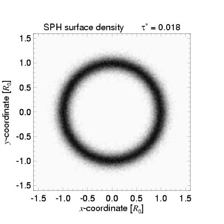
Figure 1: Evolution of the surface density of the viscous dust ring in an SPH simulation. Parameters of the disc are $R_{0}=1\,R_{\odot}$, disc mass $M=10^{-10}\,M_{\odot}$, central mass $M_{\mathrm{c}}=1\,M_{\odot}$, and kinematic viscosity $\nu_{s}=3\times 10^{-8}R_{\odot}^{2}/\mathrm{s}=1.5\times 10^{14}\mathrm{cm}^{2}/\mathrm{s}$. The initial density distribution at viscous time $\tau^{*}=0.018$ is shown in the top left plot. The symmetric structures seen in the distribution at $\tau^{*}=0.054$ may be of numerical nature due to relaxation effects of the initial particle distribution. Later, the development of the spiral instability can be seen very clearly.

The simulation presented below was performed with the following parameters. The initial SPH particle distribution represents the surface density (8) of the analytic solution at the viscous time $\tau^{*}=0.018$, with $R_{0}=1\,R_{\odot}$, disc mass $M=10^{-10}\,M_{\odot}$, and central mass $M_{\mathrm{c}}=1\,M_{\odot}$. The kinematic viscosity was set to $\nu_{s}=3\times 10^{-8}R_{\odot}^{2}/\mathrm{s}=1.5\times 10^{14}\mathrm{cm}^{2}/\mathrm{s}$ throughout the whole simulation. The initial distribution consists of 40 000 particles which are arranged symmetrically to make sure that at the beginning the centre of mass lay exactly at the origin. Due to the stochastic nature of the SPH method, no further seed perturbations are required to bring potential instabilities to grow.

Fig. 1 shows the evolution of the viscous ring during the SPH simulation in a sequence of plots of the surface density distribution. The top left plot represents the initial density distribution at viscous time $\tau^{*}=0.018$. Immediately after the start of the simulation, symmetric structures develop, which can still be seen in the distribution at $\tau^{*}=0.054$ in the top middle panel. These narrow ring-like structures may be numerical artifacts due to the relaxation of the initial particle distribution, or they may be caused by the radial viscous overstability discussed e.g. in Kley et al. (1993), but they vanish in the further course of the simulation. Instead, the development of a spiral pattern begins, in this case at the inner edge of the disc, until finally a distinct spiral structure is covering the whole face of the disc, as can clearly be seen in the distribution at $\tau^{*}=0.270$ in the bottom right panel of Fig. 1.

Figure 2: Time evolution of the first four Fourier modes at $R=R_{0}$ of the simulation shown in Fig. 1. Because of the symmetric initial particle distribution, even modes are high and odd modes are low at the beginning. Later, all modes decrease except the $(m=1)$-mode which increases exponentially as expected. The $(m=3)$- and $(m=4)$-mode merge with the noise background of the simulation, while the $(m=2)$-mode stays slightly above the noise level. The dashed line in the top left panel gives an approximated fit of the growth of the first Fourier mode to $\sigma_{i}=1.8\times 10^{-5}\mathrm{sec}^{-1}=0.028\,\Omega(R_{0})$.

To determine the nature of the spiral structure, a Fourier analysis of the evolving ring was performed during the simulation. Fig. 2 gives the time evolution of the first four azimuthal Fourier modes ($m=1$ to $m=4$) at radius $R=R_{0}$. For small viscous times, the even modes $m=4$ and especially $m=2$ are high, while the odd modes $m=1$ and $m=3$ are low. This effect is due to the symmetric initial particle distribution and disappears eventually when the symmetry of the particle distribution is lost. Later, the ($m=1$)-mode increases exponentially, while all the other modes decrease or stay small. In particular, the ($m=3$)-mode remains in the large noise background of the simulation, which is intrinsic to the SPH method, and the ($m=4$)-modes decreases down to the noise background (as all inspected higher modes do). The $(m=2)$-mode seems to end at a level slightly above the noise background, although this is not clearly to determine because of the large oscillations of the modes which are also caused by the SPH noise level.

The results of the Fourier analysis, i.e., the development of a dominant one-armed spiral structure with an additional weaker component of a two-armed spiral structure, are in complete agreement with the theoretical results of the first and second order perturbation analysis as derived in 3.4 and 3.5.

Figure 3: Ratio of the amplitudes of the errors of azimuthal and radial velocities at $\tau^{*}=0.270$ for the disc shown in the bottom right panel of Fig. 1. Plotted is the azimuthally averaged relation $|v_{\varphi}-v_{\mathrm{Kepler}}|/|v_{R}-v_{\mathrm{spreading}}|$ over radius, where $v_{\varphi}$ and $v_{R}$ are the simulation results and $v_{\mathrm{Kepler}}$ and $v_{\mathrm{spreading}}$ are the velocities (9) and (11) of the analytic solution. The curve roughly matches the expected value of $\frac{1}{2}$ (dotted line).

Figure 4: Absolute value of the phase shift between the errors of azimuthal and radial velocities, $v_{\varphi}-v_{\mathrm{Kepler}}$ and $v_{R}-v_{\mathrm{spreading}}$, for the disc at $\tau^{*}=0.270$ shown in the bottom right panel of Fig. 1, azimuthally averaged and plotted over radius. The curve roughly matches the expected value of $\frac{\pi}{2}$ (dotted line).

Further predictions of the perturbation analysis in Sect. 3, that can be tested easily, are the relations between the first order velocities $v_{R1}$ and $v_{\varphi 1}$. According to (45), their amplitudes have a ratio of 2, and they obey a phase shift of $\frac{\pi}{2}$. To verify this, we more thoroughly studied the most evolved particle distribution of the SPH simulation presented in Fig. 1, i.e. the ring at viscous time $\tau^{*}=0.270$, whose density distribution is shown in the bottom right panel of Fig. 1. In Fig. 3 the relation $|v_{\varphi}-v_{\mathrm{Kepler}}|/|v_{R}-v_{\mathrm{spreading}}|$ is plotted over radius. Here, $v_{\varphi}$ and $v_{R}$ denote the simulation results, which are averaged azimuthally using the SPH formalism, and $v_{\mathrm{Kepler}}$ and $v_{\mathrm{spreading}}$ are the velocities according to the analytic solutions (9) and (11) of the viscous ring model. Taking $v_{\varphi}-v_{\mathrm{Kepler}}\approx v_{\varphi 1}$ and $v_{R}-v_{\mathrm{spreading}}\approx v_{R1}$, the curve in diagram 3 matches the value $\frac{1}{2}$ sufficiently to satisfy relation (45). Accordingly, Fig. 4 shows the phase shift between $v_{\varphi}-v_{\mathrm{Kepler}}$ and $v_{R}-v_{\mathrm{spreading}}$, and again the plot matches the expected value of $\frac{\pi}{2}$ satisfactorily.

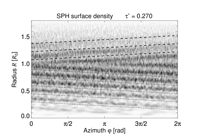
Figure 5: Surface density distribution of the disc at $\tau^{*}=0.270$ as shown in the bottom right panel of Fig. 1 but plotted in polar coordinates (radius $R$ over azimuth $\varphi$) instead of Cartesian coordinates. Additionally, lines of constant $kR\pm\varphi$ with $k=42R_{0}^{-1}$ are drawn in around $R\approx R_{0}$. Note that the spiral structure consists of a leading and a trailing spiral.

Finally, we want to compare the local stability analysis and the resulting dispersion relation established in Sect. 4 with the SPH simulation results. From the top left panel of Fig. 2, the growth rate at radius $R=R_{0}$ of the first Fourier mode may be estimated to $\sigma_{i}=1.8\times 10^{-5}\mathrm{sec}^{-1}=0.028\,\Omega(R_{0})$, the latter measured in units of the angular velocity (10) at $R=R_{0}$. With dispersion relation (75), the corresponding wave number can be estimated to $k=42R_{0}^{-1}$, which results in a wavelength of $\lambda=0.15R_{0}$. Comparing that result with the surface density distributions of Fig. 1 shows good agreement. That can be seen in particular in Fig. 5, where the surface density distribution of the ring at viscous time $\tau^{*}=0.270$ is plotted in polar coordinates, and where additionally lines of constant $kR\pm\varphi$ with $k=42R_{0}^{-1}$ are drawn in for the region around $R\approx R_{0}$. The lines match well the slopes and the wavelengths of the spiral structures. Note by the way that in this presentation of the surface density clearly can be seen that in this case the spiral structure consists of a leading (outer part of the disc) and a trailing (inner part of the disc) spiral.

5.2 Using a finite difference method

5.2.1 Numerical considerations

In addition to the particle simulations above we performed runs using a finite difference method for solving the hydrodynamic equations. The code is based on the hydrodynamic program RH2D suited to study general two-dimensional systems including radiative transport (Kley, 1989). RH2D uses a fixed Eulerian grid and is a spatially second order accurate, mixed explicit and implicit method. Due to an operator-splitting approach, the method is partly centred in time and is therefore also in time in real terms of higher accuracy than the formal first order. The advection is computed by means of the second order monotonic transport algorithm, introduced by van Leer (1977), which guarantees global conservation of mass and angular momentum. Advection and forces are solved explicitly, while the viscosity is treated either explicitly or implicitly. The formalism for application to thin discs in $(R-\varphi)$ geometry has been described in detail in Kley (1998, 1999).

To model the viscously evolving ring we work in cylindrical coordinates and solve exactly the hydrodynamic equations as given in Eqs. (1) to (3), using the full viscous stress tensor presented in (4) to (6), using an extremely small pressure with $c_{\mathrm{s}}/v_{\mathrm{Kepler}}\approx 10^{-8}$. The equations are solved in dimensionless units using an arbitrary basic unit length $R_{0}$. The unit of time $t_{0}$ is chosen such that

$$t_{0}=\sqrt{\frac{R_{0}^{3}}{GM_{\mathrm{c}}}}\quad,$$ (78)

i.e. in these units $GM_{\mathrm{c}}=1$, and the period of one Keplerian orbit at (the dimensionless radius) $R=1$ is $P_{0}=2\pi$. The only relevant physical constant entering the equations is the dimensionless coefficient of the kinematic viscosity $\nu_{s}$, which is measured in units of $\nu_{0}=R_{0}^{2}/t_{0}$.

All the grid-based models presented in this paper use the same computational domain ${\cal D}$ represented by $[R_{\mathrm{min}},R_{\mathrm{max}}]\times[\varphi_{\mathrm{min}},\varphi_{\mathrm{max}}]$ with $R_{\mathrm{min}}=0.2$, $R_{\mathrm{max}}=1.8$, $\varphi_{\mathrm{min}}=0.0$ and $\varphi_{\mathrm{max}}=2\pi$. The ring ${\cal D}$ is covered in the basic model by $128\times 128$ grid cells. However, to analyse resolution and numerical effects we use different griddings ranging from $64\times 128$ to $256\times 733$. For our basic reference model we use for the constant dimensionless viscosity $\nu_{s}=4.77\times 10^{-5}$, which is in fact identical to the value used in the particle simulations.

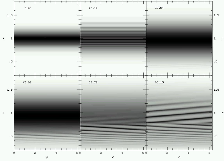
Figure 6: Grey-scale plot of the density in polar coordinates at different evolutionary times for a model with a $256\times 256$ resolution. Times are indicated in orbital periods $P_{0}$ at $R=1R_{0}$. To compare with Fig. 1: One viscous time refers to $278P_{0}$. The time evolution of the system proceeds similar to the particle simulations. In the initial phase axisymmetric perturbations are seen first ($t=17.45$). They vanish later, and the system returns to axisymmetry ($t=30.54$). Then, from the inner parts the instability develops as a trailing spiral. At the end of the simulation a leading spiral appears in the outer region of the ring.

The initial setup consists of an axisymmetric density profile following the analytic density $\Sigma_{\mathrm{ring}}$ as given in Eq. (8). Because the original $\delta$-function distribution is hard to represent numerically, we start, as above, with an initial density profile given here by the analytic solution at the viscous time $\tau^{*}=0.016$, i.e. $\Sigma(t=t_{\mathrm{init}},x=R/R_{0})=\Sigma_{\mathrm{ring}}(\tau^{*}=0.016,x)$. The slight difference to the value 0.018, used in the SPH calculations, is of no importance for the subsequent evolution. For the standard viscosity $4.77\times 10^{-5}$ this refers to the initial (dimensionless) time $t_{\mathrm{init}}=\tau^{*}R_{0}^{2}/(12\nu_{\mathrm{s}})=4.34P_{0}$. Stated differently, one viscous evolution time corresponds to 278 orbital periods $P_{0}$ for the given viscosity. The total dimensionless mass $M$ in the disc is normalised to unity. The initial radial velocity is set to zero and the angular viscosity to $v_{\mathrm{Kepler}}$.

The code is written such that axial symmetry is preserved exactly for an explicit viscosity-solver, i.e. purely axisymmetric initial conditions remain exactly axisymmetric. Hence, the initial density is disturbed randomly by typically $1$ or $0.1\%$ to supply seed perturbations, and the subsequent longterm integration has to follow the evolution on a viscous timescale which is typically about $\approx 100$ orbital periods for the standard model.

5.2.2 The standard model

An analysis of the properties of the standard model is presented. This refers to fixed physical parameter and initial conditions as outlined in the previous section. Starting from the disturbed axisymmetric density distribution the configuration evolves as presented in Fig. 6 where the density distribution is plotted for a model with a resolution of $256\times 256$ and an initial density perturbation of $0.1\%$. During the initial phase axisymmetric disturbances appear which vary on short dynamical timescales. These radial oscillations may be related to the viscous overstability discussed for example in Kato (1978) or in Kley et al. (1993). The oscillations are damped however, and the system becomes axially symmetric again. Apart from these initial variations, there are no further indications of a variation on the dynamical timescale during the remaining evolution. At $t\approx 35$ a trailing one-armed spiral density wave becomes visible in the inner parts of the ring (at $R\approx 0.4R_{0}$) which propagates slowly outwards. At later times a leading spiral appears in the outer parts of the ring which has a negative density gradient. This is in very good agreement with the SPH simulations presented above, and with the analytical results which indicated the possibility of leading and trailing waves. The outer leading spiral is not as tightly wound as the trailing inner one. That is, the radial wave number of the outer wave is smaller than the one on the inner side. This different behaviour may be caused by a wrapping up of the inner spiral by the differential rotation. At a given radius the radial separation of two wave crests (tightness of the spiral) is approximately constant with time, while for a given snapshot (time) there appears to be the tendency for the spirals to widen for larger radii.

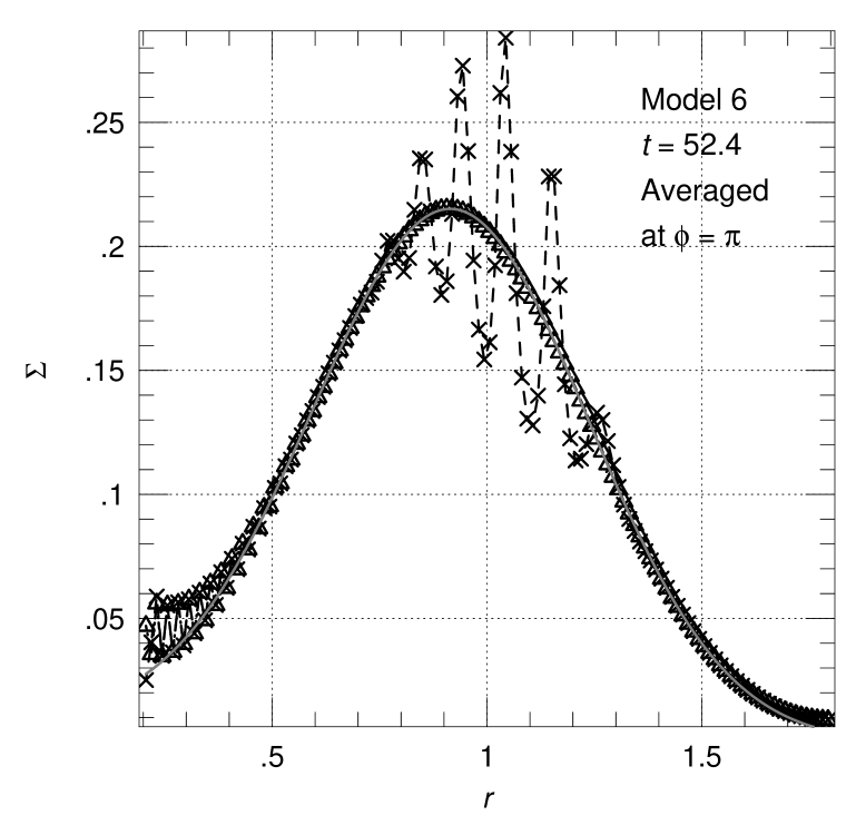
Figure 7: Radial density distribution at $\varphi=\pi$ (crosses) and azimuthally averaged (triangles). The averaged distribution follows exactly the analytical zero order result of the diffusion equation $\Sigma_{\mathrm{ring}}$, Eq. (8). Time is given in orbits at $R=1R_{0}$.

In Fig. 7 a radial cut through the density at the fixed angle $\varphi=\pi$ (crosses) is shown for the standard model ($128\times 128$ grid points), for $t=52.4$. Clearly seen are the different crests of the spirals. The radial wavelength $\lambda=2\pi/k$ of the spiral is of the order of a few grid points only. Overlaid we plotted the azimuthally averaged density profile (triangles) which follows exactly the analytical solution (solid line). This feature of the averaged density is a result of the modal form $\propto\,\mathrm{e}^{im\varphi}$ of the developing spiral structure. The oscillations at the inner boundary are caused by the artificial inner boundary condition which allows for no outflow ($v_{R}=0$ at $R_{\mathrm{min}}$) for this particular model. Opening the inner boundary yields smooth density distributions. The obtained growth rates are, however, not influenced by the exact boundary conditions, as long as the density there remains small with respect to the central density.

Figure 8: Time evolution of the first 5 azimuthal modes for the standard model measured at the radius $R=1$.

In Fig. 8 the growth rates for the first 5 modes $m=1$ upto $m=5$ are displayed. The vertical axis refers to the decimal logarithm of the amplitude. Clearly seen is the random initial perturbation at the level of $1\%$ which is reflected in a start of all modes at the level of $10^{-3}$. During the initial evolution the rings spreads slowly, the amplitudes decline until at later times ($t=15-20$) the $m=1$ mode begins to grow exponentially with time. From the plot and additional runs we may approximately determine the growth rate $\sigma_{i}=\mathrm{Im}(\sigma)$ for this $m=1$ mode of the standard model to be

$$\sigma_{i}\approx 0.035\,\Omega(R=1)\quad.$$

This is stated in units of the dimensionless time which is identical to the Keplerian orbital frequency $\Omega$ at the radius $R=1R_{0}$. To verify the numerical robustness of this result we varied several numerical parameter such as rotating frame, implicit viscosity, directional splitting, inner and outer boundary conditions, and found no significant variation.

Of course, since the growth rate $\sigma_{i}=\sigma_{i}(k)$ depends on the azimuthal wave number $k$ and thus on the grid size as well, we do expect a dependence on the numerical resolution.

Figure 9: Time evolution of the logarithm of $m=1$ mode (measured at $R=1R_{0}$) for models with varying resolution in the angular direction. The radial number of grid points is fixed to 128.

Figure 10: Time evolution of the total radial kinetic energy (dimensionless units) in the system for different numerical resolution, as indicated by the labels. The physical parameter of the models are those of the standard model.

Figure 11: Time evolution of the asymmetry $\Delta\Sigma$, Eq. (79), for different kinematic viscosities. Starting from the reference value (standard, $\nu=4.77\times 10^{-5}$) we lowered and increased the value of $\nu$ by the factors given in the key.

Figure 12: The growth rates (in units of $\Omega$ at $R=1$) versus kinematic viscosity in units of the standard viscosity ($4.77\times 10^{-5}$) for different kinematic viscosities and for both numerical methods.

5.2.3 Varying resolution and viscosity

To test the influence of the numerical resolution we first fixed the number of grid points in the radial direction (to 128) and then varied the number of the angular grid points (from 128 to 370). The results in Fig. 9 indicate that the growth rate of the $m=1$ mode (measured at $R=1R_{0}$) is nearly independent of the resolution in $\varphi$ and converges for large $N_{\varphi}$ to one value. This is consistent with our result that to second order the growth rates should be independent of the azimuthal wave number $m$.

In the next set of models the number of radial grid points was allowed to vary as well. The time evolution of the total radial kinetic energy is displayed in Fig. 10 for models with different radial (and azimuthal) grid resolutions. For very small radial resolutions $N_{R}=64$ there is very little or no growth. Then, for an increasing number of radial grid points the growth rates increase as well. This effect of faster growth for higher resolution is not an artifact of the numerical analysis but is to be expected from our analytical estimates. It was shown that the growth rates $\sigma$ depend on the radial wave number $k$: The smaller the wavelength of the perturbation the faster the growth rates. But the smallest wavelength that can be resolved by numerical computations depends naturally on the resolution. Notice, that the wave crests in such a simulation are always resolved by only a few grid cells (see Fig. 7).

To study the influence of the kinematic viscosity we varied $\nu$ from the standard value to higher and smaller values. In Fig. 11 results are shown for several models. A measure of the global deviation $\Delta\Sigma$ of the density from the axisymmetric structure has been plotted, with $\Delta\Sigma$ defined as

$$\Delta\Sigma=\max_{\cal D}\left(\frac{\Sigma(r,\,\varphi)-\Sigma(r,\,\varphi+\pi)}{\Sigma(r,\,\varphi)+\Sigma(r,\,\varphi+\pi)}\right)$$ (79)

where the maximum is taken over the whole computational domain ${\cal D}$. This measurement of $\Delta\Sigma$ is often a better tool to analyse the growth rates than just studying the $m=1$ mode at some specific radius as done above.

It can be seen that upon increasing the viscosity the growth rates are also increasing, which is again in agreement with our analytical estimates. The initial increase of $\Delta\Sigma$ for the two models with the lowest viscosities ($\nu_{s}$ and $1/2\;\nu_{s}$) is related to the nearly ring like disturbances described before. These decline first, and then later the growth of the spiral disturbance sets in. The exact behaviour of the curves depends on the initial random perturbation as well.

Finally we display the obtained growth rates for different viscosity coefficients in Fig. 12, where the solid line denotes the results computed by the finite difference method. For larger viscosities the growth rates are also larger which is in agreement with Eq. (75). To compare exactly with the analytical results, the wavelength of the most unstable mode needs to be known as well. However, the wave number is a function of radius, making a detailed comparison not as easy. It is found in general that the obtained growth rates (as given for example in Fig. 12) are in the right order with the first term of Eq. (75) but are consistently lower. The radial variation of the quantities may easily account for this slight discrepancy.

Additionally, results of similar SPH calculations are plotted in Fig. 12, indicated by the dashed line. In all cases, the SPH results fit the dispersion relation (75) well within the accuracy of the SPH simulations. However, the growth rates as well as the associated wave numbers of the most unstable mode are lower than the grid-based results. Moreover, the growth rate increases slower with increasing viscosity. This behaviour may demonstrate that the relation of growth rate and wave number is depending on spatial resolution, initial condition, and on the numerical method. The discrepancy may also be caused by different evaluation methods. While for the SPH results the growth rates were measured locally from the evolution of the amplitude of the $m=1$ Fourier mode at radius $R=R_{0}$, for the grid-based results they were determined globally by analysing the change of $\Delta\Sigma$ according to Eq. (79). This may also be another cause why the grid-based results fulfil the dispersion relation (75) not exactly.

6 Conclusion

We have shown that the spiral instability found in various simulations of the viscously evolving dust ring can be understood in terms of a secular spiral instability driven by viscosity. To accomplish this, we performed a perturbation analysis using a time-stretching transformation. It turned out that the widely known analytic solutions for the surface density evolution and the azimuthal velocity of the viscously spreading ring consist of the zeroth order terms of the expansion, while the solution for the radial velocity is given by the 1st order terms.

As a result of the perturbation analysis we found that the ring may develop one-armed spiral structures to 1st order and one- and two-armed spiral features to 2nd order. A local stability analysis of an eccentricity function $E$ provided a dispersion relation that led for a constant kinematic viscosity to a growth rate for secular spiral instabilities of

$$\sigma_{i}=\frac{1}{3}\,k^{2}\,\nu\,+\,\mathcal{O}(\nu/R^{2})$$

in the limit $kR\gg 1$. The exact form of the growth rate depends on the viscosity prescription $\nu=\nu(R)$. Our theoretical results could be confirmed in several simulations using two different numerical methods.

As a consequence for numerical simulations of accretion discs, the spiral instability has to be taken into account when using the spreading ring for instance as test problem for code development. Otherwise, occasionally emerging spiral features may be mistaken for numerical instabilities of the algorithms used for the calculation of the viscous forces.

The physical implications of our results are not as obvious. Because the kinematic viscosity $\nu$ is held axisymmetric throughout the whole stability analysis, the discovered non-axisymmetric instabilities may be of importance mainly in accretion discs where the viscosity is determined uniformly by external effects like irradiation.

References

• Flebbe et al. (1994) Flebbe, O., Münzel, S., Herold, H., Riffert, H., & Ruder, H. 1994, ApJ, 431, 754
• Frank et al. (2002) Frank, J., King, A., & Raine, D. 2002, Accretion power in astrophysics (Cambridge University Press)
• Gingold & Monaghan (1977) Gingold, R. & Monaghan, J. 1977, MNRAS, 181, 375
• Kato (1978) Kato, S. 1978, MNRAS, 185, 629
• Kley (1989) Kley, W. 1989, A&A, 208, 98
• Kley (1998) —. 1998, A&A, 338, L37
• Kley (1999) —. 1999, MNRAS, 303, 696
• Kley et al. (1993) Kley, W., Papaloizou, J. C. B., & Lin, D. N. C. 1993, ApJ, 409, 739
• Lucy (1977) Lucy, L. 1977, AJ, 82, 1013
• Lüst (1952) Lüst, R. 1952, Z. Naturforschg., 7a, 87
• Lynden-Bell & Pringle (1974) Lynden-Bell, D. & Pringle, J. E. 1974, MNRAS, 168, 603
• Maddison et al. (1996) Maddison, S. T., Murray, J. R., & Monaghan, J. J. 1996, Publications of the Astronomical Society of Australia, 13, 66
• Monaghan (1992) Monaghan, J. J. 1992, ARA&A, 30, 543
• Monaghan & Gingold (1983) Monaghan, J. J. & Gingold, R. 1983, Journal of Computational Physics, 52, 374
• Ogilvie (2001) Ogilvie, G. I. 2001, MNRAS, 325, 231
• Pringle (1981) Pringle, J. E. 1981, ARA&A, 19, 137
• Riffert et al. (1995) Riffert, H., Herold, H., Flebbe, O., & Ruder, H. 1995, Computer Physics Communications, 89, 1
• Speith & Riffert (1999) Speith, R. & Riffert, H. 1999, Journal of Computational and Applied Mathematics, 106, 231
• van Leer (1977) van Leer, B. 1977, Journal of Computational Physics, 23, 276