Small-scale structure of the galactic cirrus emission

We examined the Fourier power spectrum characteristics of cirrus structures in 13 sky fields with faint to bright cirrus emission observed with ISOPHOT in the 90–200$\mu$m wavelength range in order to study variations of the spectral index $\alpha$. We found that $\alpha$ varies from field to field with –5.3 $\leq$ $\alpha$ $\leq$ –2.1. It depends on the absolute surface brightness and on the hydrogen column density. We also found different spectral indices for the same sky region at different wavelengths. Longer wavelength measurements show steeper power spectra. This can be explained by the presence of dust at various temperatures, in particular of a cold extended component. For the faintest areas of the far-infrared sky we derive a wavelength independent spectral index of $\alpha$ = –2.3$\pm$0.6 for the cirrus power spectrum. The application of the correct spectral index is a precondition for the proper disentanglement of the cirrus foreground component of the Cosmic Far-Infrared Background and its fluctuations.

1 Introduction

                      
                       Figure 1: 100 and 200 $\mu$m range images of two sample fields in the satellite coordinate system (Laureijs et al., 2002). The central sky positions of the images are listed in Table 1. The orientation of the celestial coordinate system is indicated. (a) Cham–II, 200 $\mu$m (b) Cham–II, 100 $\mu$m (c) NPC 1, 200 $\mu$m (d) NPC 1, 90 $\mu$m. While the FIR emission in NPC 1 arises from the same cirrus structure at both wavelengths, there seems to be an additional component of cold condensations in Cham II, as discussed in Sect. 5.1.

In the far-infrared the most significant component superimposed on the Extragalactic Background is the cirrus emission of the Galaxy originating from irregularly shaped interstellar clouds (Low et al., 1984). The correct determination of the Cosmic Far-InfraRed Background (CFIRB) requires a precise removal of this foreground component (Guiderdoni et al., 1997). The CFIRB is characterized by two parameters: the absolute level and the amplitude of its fluctuations. In recent years observations made by ISOPHOT (Lemke et al., 1996), the photometer on board the ISO satellite (Kessler et al., 1996) made the determination of the CFIRB fluctuations possible.

CFIRB fluctuations are expected to show the following properties (see e.g. Hauser & Dwek, 2001): (1) the spatial distribution corresponds to a flat power spectrum, (2) they are isotropic and (3) they have a positive constant value. In contrast, the fluctuations due to galactic cirrus emission scale up with absolute brightness and can be described by a multifractal structure, yielding a steep Fourier power spectrum. It is usually described by one main parameter, the spectral index $\alpha$:

$$\rm P=P_{0}\times(f/f_{0})^{\alpha}$$ (1)

where P is the Fourier power, f is the absolute value of the two-dimensional spatial frequency and P₀ is the Fourier power at the spatial frequency f₀ (Gautier et al., 1992). Since cirrus fluctuations are different from CFIRB fluctuations in at least two features (spatial frequency– and brightness–dependence), it is possible to separate them from each other in two independent ways:

(1) The decomposition through the brightness dependence at a fixed spatial frequency was performed by Kiss et al. (2001, hereafter Paper I), and resulted in a new determination of the CFIRB fluctuation amplitudes at 90 and 170 $\mu$m.

(2) The decomposition using the Fourier power spectrum was introduced by Guiderdoni et al. (1997). For faint fields, where CFIRB fluctuations are expected to be dominant in the highest spatial frequency range, the knowledge of the cirrus spectral index is mandatory for decomposition. Gautier et al. (1992) determined a spectral index of the galactic cirrus emission $\alpha$ $\approx$ –3 from the analysis of 100 $\mu$m IRAS scans. For regions of faint total FIR brightness emission Lagache & Puget (2000) and Matsuhara et al. (2000) derived CFIRB fluctuation amplitudes applying this spectral index of $\alpha$ $\approx$ –3 for the cirrus decomposition.

Herbstmeier et al. (1998) analysed a few fields observed by ISOPHOT in the 90–180 $\mu$m wavelength range. They found a variation of spectral indices in the range of –0.5 $\geq$ $\alpha$ $\geq$ –3.6, depending on wavelength, brightness and sky position. However, this sample was too small (four fields, two of them measured only at one wavelength) for general conclusions, but their results clearly indicated that the $\alpha$ = –3 cirrus spectral index may not be universal.

Despite the strong impact of the cirrus power spectrum on the correct determination of the characteristics of the CFIRB, cirrus power spectrum properties were not yet analysed in detail for $\lambda$ $>$ 100$\mu$m and at a resolution achievable by ISOPHOT. In this paper we analyse 13 sky regions measured by ISOPHOT in the 90–200 $\mu$m range and investigate the characteristics of their Fourier power spectra.

2 Observations and data analysis

2.1 Selection of ISOPHOT maps

We selected 20 FIR maps from the ISO archive, covering 13 separate sky regions. All selected maps were obtained in the PHT22 staring raster observing mode (Laureijs et al., 2002). We excluded maps containing strong point sources or obvious spatial structures. This selection is a subsample of the fields used in Paper I. The selected maps had to show a clear sign of cirrus emission in the power spectrum. This requires a minimum average surface brightness of $\langle$B$\rangle$ $\approx$ 3 MJysr^-1. Such fields are slightly brighter than the faintest fields in the far-infrared sky ($\langle$B$\rangle$ $\approx$ 2 MJysr^-1) in the 90–200 $\mu$m wavelength range after the subtraction of the Zodiacal Light.

Our sample covers the surface brightness range $\sim$ 3–60 MJysr^-1, ranging from faint to bright cirrus, and faint molecular cloud emission. The basic properties of the maps are summarized in Table 1. Images of two fields are shown in Fig.1, more images are presented in Herbstmeier et al. (1998).

(1)

(2)

(3)

(4)

(5)

(6)

(7)

(8)

(9)

(10)

(11)

(12)

(13)

(14)

field

$\lambda$

size

field center

$\rm\langle B_{\lambda}\rangle$

$\alpha$

P0

$\delta\alpha$

${\delta}P_{0}$

W(12CO)

N(HI)

associated objects

references

($\mu$m)

(arcmin)

l

b

(MJysr-1)

(Jy2sr-1)

(Kkms-1)

(cm-2)

NGP

180

46.0$\times$46.0

88.9

73.0

3.1$\pm$0.1

–2.53$\pm$0.22

1.8$\times$103

1.59

0.95

$-$

9.0$\times$1019

North Galactic Pole

Juvela et al. (2000)

Herbstmeier et al. (1998)

Draco

90

7.7$\times$7.7

89.8

38.6

5.7$\pm$0.3

–2.45$\pm$0.17

5.3$\times$103

1.47

0.76

$-$

2.1$\times$1020

Draco nebula

Herbstmeier et al. (1998)

Draco

170

27.6$\times$18.4

89.8

38.6

4.7$\pm$0.5

–4.09$\pm$0.22

2.9$\times$103

2.71

1.39

–

2.1$\times$1020

Draco nebula

Herbstmeier et al. (1998)

Cep

90

14.7$\times$20.7

108.0

13.6

23.5$\pm$3.1

–3.42$\pm$0.15

3.3$\times$104

1.96

1.01

6.9

2.5$\times$1021

Cepheus Flare

Herbstmeier et al. (1998)

Cep

170

21.5$\times$24.5

108.0

13.6

68.2$\pm$12.7

–4.19$\pm$0.12

3.0$\times$105

1.95

1.56

6.9

2.5$\times$1021

Cepheus Flare

Herbstmeier et al. (1998)

NPC1

90

29.9$\times$29.1

121.6

24.2

7.6$\pm$0.8

–3.10$\pm$0.04

5.0$\times$103

2.16

0.64

6.6

6.9$\times$1020

Polaris Flare

Gautier et al. (1992)

NPC1

200

30.7$\times$29.1

121.6

24.2

26.1$\pm$5.3

–3.46$\pm$0.09

1.1$\times$105

2.30

0.95

6.6

6.9$\times$1020

Polaris Flare

Gautier et al. (1992)

NPC2

90

29.9$\times$29.1

122.0

24.6

7.4$\pm$0.7

–2.83$\pm$0.09

5.7$\times$103

1.74

0.89

5.5

6.7$\times$1020

Polaris Flare

Gautier et al. (1992)

NPC2

200

30.7$\times$29.1

122.0

24.6

22.6$\pm$3.8

–3.39$\pm$0.08

9.7$\times$104

2.19

0.63

5.5

6.7$\times$1020

Polaris Flare

Gautier et al. (1992)

North1

90

29.9$\times$29.9

100.0

14.8

13.3$\pm$1.4

–3.05$\pm$0.09

9.7$\times$103

1.83

0.91

4.5

1.6$\times$1021

LDN 1122

Yonekura et al. (1997)

North1

200

30.7$\times$30.7

100.0

14.8

34.4$\pm$5.6

–4.70$\pm$0.17

4.5$\times$104

2.43

0.52

4.5

1.6$\times$1021

LDN 1122

Yonekura et al. (1997)

North2

90

29.9$\times$29.9

108.0

15.2

12.4$\pm$1.8

–3.65$\pm$0.13

9.2$\times$103

1.42

0.90

6.6

2.1$\times$1021

LDN 1147, 1148

Lee et al. (2001)

Yonekura et al. (1997)

North2

200

30.7$\times$30.7

108.0

15.2

40.7$\pm$12.5

–3.81$\pm$0.09

3.2$\times$105

1.94

0.61

6.6

2.1$\times$1021

LDN 1147, 1148

Lee et al. (2001)

Yonekura et al. (1997)

M01

180

27.6$\times$27.6

100.0

30.6

5.0$\pm$0.2

–2.56$\pm$0.41

2.3$\times$102

0.89

0.75

$-$

4.2$\times$1020

faint field in Dra

Herbstmeier et al. (1998)

Ábrahám et al. (1997)

M03

180

27.6$\times$27.6

117.6

46.1

3.7$\pm$0.1

–2.12$\pm$0.23

5.8$\times$102

0.82

0.71

$-$

1.5$\times$1020

faint field in UMi

Ábrahám et al. (1997)

TMC2-1

200

30.7$\times$30.7

173.9

–15.7

56.5$\pm$8.9

–5.26$\pm$0.15

3.7$\times$105

1.74

0.86

18.9

1.7$\times$1021

LDN 1529, 1531

Lee et al. (2001)

Taurus 2 mol. cl.

Chappell & Scalo (2001)

TMC2-2

200

30.7$\times$30.7

174.3

–15.9

63.7$\pm$8.5

–3.49$\pm$0.14

3.8$\times$105

1.66

1.04

16.3

1.8$\times$1021

LDN 1529, 1531

Lee et al. (2001)

Taurus 2 mol. cl.

Chappell & Scalo (2001)

Cha1S

100

19.9$\times$19.9

297.3

–16.2

29.3$\pm$3.2

–3.80$\pm$0.08

1.4$\times$105

2.47

0.79

10.3

9.2$\times$1020

Chamaeleon mol. cl.

Tóth et al. (2000)

ChamII

100

31.4$\times$31.4

303.5

–14.2

23.9$\pm$3.3

–2.95$\pm$0.08

1.7$\times$105

0.91

0.89

16.1

1.2$\times$1021

DCld 303.3–14.3,

Tóth et al. (2000)

ChamII

200

30.7$\times$30.7

303.5

–14.2

38.4$\pm$14.6

–5.17$\pm$0.18

2.4$\times$105

2.48

0.53

16.1

1.2$\times$1021

303.5–14.4

Tóth et al. (2000)

Table 1. Basic observational and derived parameters of fields mapped by ISOPHOT. The columns are: (1) name of the field as specified by the observer; (2) central wavelength of filter; (3) map size; (4)–(5) center of the field in galactic coordinates; (6) median surface brightness from ISOPHOT photometry with Zodiacal Light subtracted; quoted standard deviations are a measure of the dynamic range of the map. (7) spectral index of the power spectrum; (8) fluctuation power at the reference spatial frequency 1/d₀ (d₀ = 4′); (9)–(10) parameters describing the relative strength of the instrument noise power spectrum to the signal power spectrum (see Eq. 2 for the definitions); (11) average neutral hydrogen column density (Dickey & Lockman, 1990); (12) ¹²CO integrated intensity (Dame et al., 2001); (13) associated objects or dark clouds located (at least partially) inside the field. (14) references with the description of the field.

2.2 Data reduction

We used the final maps produced for the confusion noise analysis in Paper I. For a detailed description of the data reduction steps we refer to this paper. The data reduction comprised the following main steps:

• Basic data analysis with PIA V8.2 (Gabriel et al., 1997) from ERD to AAP level

• Flat-fielding using first quartile normalization

• Subtraction of the Zodiacal emission

2.3 Fourier power spectrum

Fourier transformation of the maps was performed by routines written in IDL based on the standard IDL FFT routine with periodogram normalisation (Press et al., 1992). For all maps the highest spatial sampling frequency corresponds to the pixel size of the C100 and C200 array cameras. The Nyquist limit which allows correct sampling (without aliasing) is half of that frequency (Press et al., 1992, Chapter 12.1), i.e. the double pixel size of the array. Therefore, the upper limit of the spatial frequency considered for the Fourier power spectrum was set to the Nyquist-limit, which is $\theta_{min}$ = 92″  for images with $\lambda$ $\leq$ 100 $\mu$m (C100 detector) and $\theta_{min}$ = 184″ for images with $\lambda$ $>$ 100 $\mu$m (C200 detector). Since the pixel sizes of the ISOPHOT C100 and C200 cameras were adjusted to the diffraction limit, this limit should be kept, even if the raster sampling were finer than the pixel size.

Instead of averaging P(f) fluctuation power values in annuli for each f = $|$f$|$ spatial frequency, we used all individual data points (f, P(f) pairs) to derive the final power spectrum. The spectral index $\alpha$ is derived by robust line fitting to all data points in the log(f)–log(P) space.

In most cases the whole power spectrum could be satisfactorily fitted by one spectral index. For some faint fields, however, the high frequency end of the spectrum showed a different (flatter) spectral index, due to a higher structure noise level. In such cases we only used the low and mid frequency part to derive $\alpha$. The reason for this flattening will be discussed below in Sect. 4.

3 Features affecting the power spectrum

There are several contributions to the power spectrum that can affect its final shape. We analyse the effects of the instrument noise, a point-source footprint and an extended source profile on the final power spectrum. The correct separation of the power spectrum components requires well-distinguishable spectral indices, otherwise they cannot be disentangled.

3.1 Power spectrum of the instrument noise

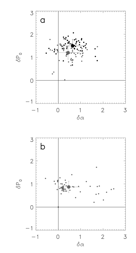
Figure 2: Relative strength of the instrument noise- to the signal power spectrum. (a) Subsample of 56 maps from Paper I., observed with the C200 detector in oversampling mode. Black dots: flat-field noise; gray dots: PIA-noise. (b) Subsample of 60 maps from Paper I., observed with the C100 detector. In this case no representative values of the flat-field noise could be dervied due to the lack of a sufficient number of oversampled maps. The average values and the standard deviations both in $\delta\alpha$ and $\delta{P_{0}}$ are marked via large dots and error bars, respectively.

Instrument noise can be a significant contribution to the fluctuation power at low surface brightness and high spatial frequencies. As discussed in detail in Paper I, the most representative estimates of the instrument noise are PIA-noise (which reflects the statistical uncertainties in signal derivation) and flat-field noise (which reflects the variation of the signal from individual detector pixels at the same sky position). Flat-field noise can only be determined for oversampled maps.

We assume that both the signal and instrument noise power spectra - derived from the surface brightness maps and the corresponding noise maps, respectively - are described by a power law behaviour as in Eq. 1. Here the $\rm f_{0}$ values correspond to the Nyquist-limits, i.e$\theta_{min}$ = 92″  and 184″  for the C100 and C200 detectors, respectively.

The signal power spectrum is not affected by the instrument noise, if the power spectrum of the instrument noise is reasonably weaker than that of the signal in the frequency range analysed. This is ensured, if two criteria are fulfilled simultaneously: (1) the fluctuation power of the instrument noise P_i is lower by at least a factor of 2 than that of the signal P$s$ at the resolution limit, $\rm\theta_{min}$ and (2) the power spectrum of the signal is steeper than that of the instrument noise. These conditions are parametrized by the following two quantities ($i$ and $s$ denote instrument noise and signal, respectively):

$$\rm\delta\alpha=\alpha_{i}-\alpha_{s}>0\leavevmode\nobreak\ \leavevmode\nobreak\ \leavevmode\nobreak\ \leavevmode\nobreak\ \leavevmode\nobreak\ \leavevmode\nobreak\ \delta{P_{0}}=log_{10}\bigg{(}{{P_{0}^{s}}\over{P_{0}^{i}}}\bigg{)}>0.3$$ (2)

For the instrument noise analysis we used a larger sample of maps than for the cirrus power spectrum study. In Table 1 we provide the respective values of $\delta\alpha$ and $\rm\delta P_{0}$ for our special fields, which can be compared with the ranges of $\delta\alpha$ and $\rm\delta P_{0}$ for the larger sample of maps.

In the case of the C200 detector we calculated $\delta\alpha$ and $\delta{P_{0}}$ for a subsample of 56 maps from Paper I, observed with full oversampling (Fig. 2a).

Most of the flat-field and PIA-noise data points are located in the quadrant where both $\delta\alpha$ and $\delta{P_{0}}$ are positive. Although there are a few points in the negative $\delta\alpha$ regime, they are close to zero, representing nearly parallel instrument noise and signal power spectra. Since in all cases $\delta{P_{0}}$ $>$ 0.3, the instrument noise power spectrum does not exceed the signal power spectrum for frequencies below $\rm\theta_{min}^{-1}$. The data points with $\alpha\,\la\,0$ belong to the faintest regions of the sky with a nearly flat power spectrum, showing no signs of cirrus ($\rm\alpha_{s}$ and $\alpha_{i}\approx$ 0). The distributions of the PIA- and flat-field noise data points are rather similar, and the average values are within the standard deviations in $\delta\alpha$ and $\delta{P_{0}}$ (big black and gray dots with error bars in Fig. 2a). This demonstrates that the method of noise determination has no impact on the final result.

In the case of the C100 detector it was not possible to perform a similar investigation due to the lack of suitable oversampled maps. Therefore, we analysed 60 observations from Paper I by calculating the PIA-noise values only (Fig. 2b). Also the C100 detector measurements fulfil the requirements of a suitable signal-to-noise ratio.

This noise analysis justifies, that for both C200 and C100 maps of Table 1 instrument noise does not affect the final shape of the power spectrum, in particular since for all of them $\delta\alpha$ $>$ 0.8 and $\delta{P_{0}}$ $>$ 0.5.

3.2 Power spectra of point- and extended sources

Figure 3: Schematic representation of the contribution of different emission components to the final power spectrum. (a) Convolution of a theoretical cirrus spectrum of arbitrary stength ($\alpha$ = –3, P = 10³ Jy²sr^-1 at f = 0.1 arcmin^-1) with ISOPHOT’s theoretical point-source footprint at 90 $\mu$m (dashed line) and at 200 $\mu$m (dash-dotted line). The pure, non-convolved cirrus spectrum is also shown (solid line). (b) Resulting power spectrum of a cirrus-like intensity distribution ($\alpha$ = –3, solid line) and an extended source of Gaussian shape with a FWHM of 1/6 (dotted line) and 1/3 (dash–triple-dotted line) of the size of the original map. The Gaussians are normalized to P = 10⁵ Jy²sr^-1 at f = 0 arcmin^-1. The Nyquist-limits for the C100 and C200 filter maps are marked both in (a) and (b) by vertical dashed and dash-dotted lines, respectively.

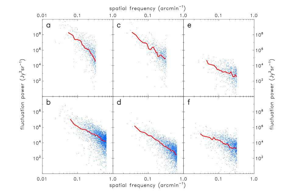
Figure 4: Power spectra of six sample fields, two of them observed by both the C100 and the C200 camera. The images corresponding to the first four power spectra are presented in Fig. 1. Images of M01 and NGP can be found in Herbstmeier et al. (1998). (a) Cham–II, 200 $\mu$m (b) Cham–II, 100 $\mu$m (c) NPC 1, 200 $\mu$m (d) NPC 1, 90 $\mu$m (e) M01, 180 $\mu$m (f) NGP, 180 $\mu$m. Each dot represents a (f,P(f)) pair, the solid line is smoothed average to outline the trend. The high frequency end is determined by the Nyquist-limit, the low frequency end by the size of the map.

In Fig. 3a we present a model cirrus spectrum with an expected cirrus spectral index of $\rm\alpha\,=\,-3$ convolved with the 90 $\mu$m and 200 $\mu$m theoretical footprints (footprint = convolution of the telescope point spread function with the pixel aperture, Laureijs et al., 2002). This figure shows, that the footprint has only a little effect below the actual Nyquist-limit, and this effect can be neglected when deriving the spectral index. A strong point source may dominate the whole spectrum, but maps containing these features were not included in our sample.

As will be shown in Sect. 5.1, extended sources with excess emission may be superimposed on the cirrus-like intensity distribution. We tested the effect of these sources on the power spectrum assuming a Gaussian shape, and a FWHM of 1/3 and 1/6 of the size of the original map, respectively, as presented in Fig. 3b. The shape of the resulting power spectrum strongly depends on the relative strength of the cirrus and extended source components. The typical effect of the extended source is the appearance of a ’hump’ at medium spatial frequencies, if the strengths of the two components are comparable. Similar (however weaker) features can be identified in some of our real power spectra, especially at 200 $\mu$m (see Fig. 4). The high frequency part of an extended source power spectrum is rather steep and therefore – if dominant – can lead to a power spectrum steeper than the one of pure cirrus. A set of extended sources has a power spectrum similar to that of a single one, but the higher the number of sources, the shallower the final power spectrum. In certain configurations these spectra may be described by an average spectral index of $\alpha$ $\approx$ –3, leading to a spectrum, which is in practice undistinguishable from the one of cirrus.

4 Results

Table 1 and Fig. 4 present the results of the power spectrum analysis.

The fields in our analysis were characterized by the following physical parameters: median FIR surface brightness from ISOPHOT photometry with Zodiacal Light subtracted (this work), neutral hydrogen column density (Dickey & Lockman, 1990) and ¹²CO integrated intensity (Dame et al., 2001). The power spectra follow quite well the expected power-law behaviour up to the spatial frequency corresponding to the resolution limit, and therefore can be satisfactorily fitted by one single spectral index $\alpha$. The only exceptions are the fields NGP (Fig. 4f), M01 (Fig. 4e) and M03 at 180 $\mu$m. They show a flattening of the spectrum for the highest spatial frequencies which was eventually excluded in the derivation of the $\alpha$ values given in Table 1.

We suggest that the relatively strong structure noise at high spatial frequencies arises from the fluctuations due to the extragalactic background. As discussed in Paper I, the extragalactic background is the major contributor to the structure noise at high spatial frequencies for the faintest regions of the far-infrared sky measured with the C200 detector. These three faint fields have an average surface brightness comparable to that of the cosmological fields. The extragalactic background is expected to have a fluctuation power of $\rm\sim{8\times}10^{2}$ $Jy^{2}sr^{-1}$ at 170 $\mu$m with our FFT normalization. Fluctuation powers at the reference spatial frequency listed in Table 1 (column #8) are fitted values using the cirrus-like power spectrum, therefore they can be lower than the expected CFIRB fluctuation level.

We calculated the median values of the spectral indices for the C100 and C200 fields ($\rm\overline{\alpha}_{C1}$ and $\rm\overline{\alpha}_{C2}$, respectively), in order to compare them with previous results. This resulted in $\rm\overline{\alpha}_{C1}\leavevmode\nobreak\ =\leavevmode\nobreak\ -3.15{\pm}0.48$ and $\rm\overline{\alpha}_{C2}\leavevmode\nobreak\ =\leavevmode\nobreak\ -3.87{\pm}1.06$. The median C100 spectral index is not much different from the one determined by Gautier et al. (1992) from the analysis of IRAS 100$\mu$m scans, however it shows a relatively large scatter. Abergel et al. (1996) performed a pixelwise determination of the spectral index for a 12$\aas@@fstack{\circ}$5$\times$12$\aas@@fstack{\circ}$5 ISSA map close to the South Ecliptic Pole. At 100 $\mu$m they obtained an average spectral index of $\rm\overline{\alpha}_{100}\,=\,-3.34$ (using the relation $\rm\alpha\,=\,-2(\beta-1)$ between their $\beta$-value and our spectral index). The distribution of the spectral index over the field had a Gaussian shape with $\sigma_{\alpha}$ = 0.36. This means, that within one field the variation is comparable to the variation we found for our sample fields. The C200 spectral indices are significantly steeper with an even higher scatter than the C100 spectral indices.

Spectral indices show a clear dependence both on the surface brightness and on the neutral hydrogen column density. Brighter fields and fields with higher HI column density usually have a steeper power spectrum (Fig. 5). We tested the degree of correlation by calculating the linear Pearson correlation coefficient which resulted in 0.69, 0.80 and 0.67 for the $\rm log_{10}\langle B_{C1}\rangle$–$\rm\alpha_{C1}$, $\rm log_{10}\langle B_{C2}\rangle$–$\rm\alpha_{C2}$ and $\rm log_{10}N(HI)$–$\alpha$ relations, respectively, without the data points of the Draco region (marked in Fig. 5 by an arrow).

If we exclude in Fig. 5b the three data points with high B_C2 and $\alpha$ $<$ –4.5, then the $\rm log_{10}\langle B_{C2}\rangle$–$\rm\alpha_{C2}$ correlation is much tighter with a linear Pearson correlation coefficient of 0.94. This exclusion is justified by the fact, that all three fields have a high HI column density and two of them show a large $\alpha_{C2}$/$\alpha_{C1}$ ratio (Fig. 5c), indicative of a relatively large molecular hydrogen content, as discussed below in Sect. 5.2.

It is possible to determine an $\alpha_{C2}$ value for the faintest fields of the far-infrared sky, by a robust linear extrapolation of the $\rm log_{10}\langle B_{C2}\rangle$–$\rm\alpha_{C2}$ relation. In order to account for the contribution by the CFIRB the B_C2 values were reduced beforehand by 0.8 MJysr^-1 (Paper I). For all points except the Draco region this resulted in $\alpha_{C2}$ = –2.3$\pm$0.6 for the faintest cirrus fields ($\langle B\rangle$ $\approx$ 2 MJysr^-1). Excluding in addition the three points with $\alpha$ $<$ –4.5, $\alpha_{C2}$ = –2.1$\pm$0.4. The impact of this power law in separating the CFIRB from the galactic cirrus is discussed in Sect. 5.3.

Figure 5: Relationship of the spectral index with (a) the 100 $\mu$m range (90–100 $\mu$m) median surface brightness B_C1, (b) the 200 $\mu$m range (170–200 $\mu$m) median surface brightness B_C2, (c) the average neutral hydrogen column density. Crosses and open circles mark fields observed at $\lambda$ $\leq$ 100 $\mu$m and 170 $\leq$ $\lambda$ $\leq$ 200 $\mu$m, respectively. The data points of the Draco 170 $\mu$m field are marked by arrows. Error bars in (a) and (b) represent the standard deviations in B_C1 and B_C2 and they mark the errors in fitting the spectral index in $\alpha$.

In Fig. 6 we plot the ratio of the spectral indices $\rm\alpha_{C2}$/$\alpha_{C1}$ determined both for a C200 and a C100 map of the same field.

Figure 6: Ratio of the spectral indices of sky regions measured in both a long wavelength (170-200 $\mu$m, $\rm\alpha_{C2}$) and at short wavelength (90–100 $\mu$m, $\rm\alpha_{C1}$) filter versus the average surface brightness in the C100 filter (90 or 100$\mu$m, B_C1). The regions are labelled by the names as given by the observer and as listed in Table 1.

Assuming that the FIR radiation at 100 and 200 $\mu$m is emitted by the same structures the ratio $\rm\alpha_{C2}/\alpha_{C1}$ should be $\approx$ 1. It is obvious, that $\rm\alpha_{C2}/\alpha_{C1}$ varies in the range 1.0–1.8. Since the determination of the spectral index is quite accurate (see Table 1), this deviation cannot be explained by measurement uncertainties. We propose an explanation in Sect. 5.1

5 Discussion

5.1 Wavelength dependence of the spectral index

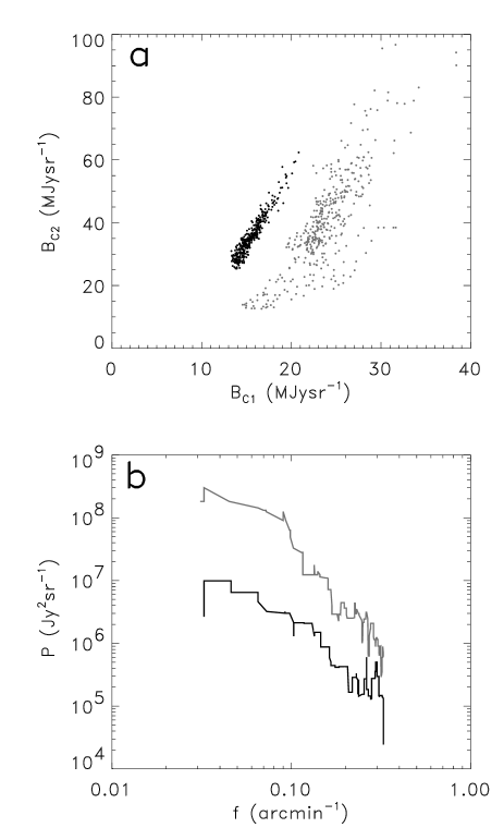
Figure 7: Examples to demonstrate the effect of a non-uniform color temperature within the same field. (a) C100 vs. C200 surface brightness scatter plots. The slope is closely related to the color temperature (see text for details). Black and gray dots represent the data points of the North 1 and Cham II fields, respectively. (b) Power spectra of the $\Delta$B images (cirrus component subtracted) of Cham II (gray) and North 1 (black).

Galactic cirrus emission is expected to have a spectral energy distribution of a modified black body, with $\nu^{2}$ emissivity law, and a dust colour temperature of 17.5$\pm$1.5 K (Lagache et al., 1998). If the FIR emission of a certain cloud can be well described by a single dust temperature, then the emission measured at two separate wavelengths should be strongly correlated, showing the same spatial structure and the same power spectrum. On the other hand, the presence of another component with different colour temperature can lead to an excess intensity at one wavelength. This yields also a different spatial structure of the emission, and therefore different power spectra at two wavelengths. Indications for such a dichotomy in cloud hierarchy were found by Abergel et al. (1996) from their analysis of the 60 and 100 $\mu$m IRAS maps of the South Ecliptic Pole field. Uncorrelated features come from the coldest regions of the analysed fields.

We tested the uniqueness of the colour temperatures for fields, where measurements at two wavelengths were available. The colour temperature is represented by the flux ratio of the two wavelengths. Two examples are presented in Fig. 7. The 90–100 $\mu$m surface brightness maps were smoothed to the resolution of the 170–200 $\mu$m measurements in order to produce B_C1 – B_C2 pixel-to-pixel scatter plots, where B_C1 and B_C2 are the surface brightnesses of the 90–100 $\mu$m and 170–200 $\mu$m map pixels, respectively. In most cases the scatter plot showed a well correlated B_C1 – B_C2 emission and could be fitted by one straight line, corresponding to one single dust temperature. Using this relation we derived an excess surface brightness $\Delta$B map, by subtracting the scaled up B_C1 emission from B_C2.

$$\Delta B\,=\,B_{C2}-[A_{1}\times B_{C1}+A_{0}]$$ (3)

where A₁ and A₀ are the slope and the interception of the linear fit to the scatter plot, respectively.

However, as presented in Fig. 7a, in some cases there was more than one characteristic colour temperature present in a field. The most conspicuous example is the Cham II field (gray dots in Fig. 7a). In this case, after removing the cirrus contribution according to the procedure of Eq. 3, the excess surface brightness image $\Delta$B still showed the steep index of the original map. The steep $\Delta$B power spectrum can be associated to a bright extended source, as suggested by the examples in Sect 3.2 and, indeed, the region contains dark cloud cores, namely DCld 303.3-14 and DCld 303.5-14.4 (see Table 1). The expected flattening at low spatial frequencies due to the extended source power spectrum (see Sect. 3.2) can also be identified. The characteristic size of the extended source derived from the power spectrum agrees well with the typical cold core extent of $\sim$10′  found by Tóth et al. (2000) in Chamaeleon, with temperatures of $\leq$ 15 K. A similar effect can be observed for the North 1 field, however, the differences are smaller than in the case of the Cham II region. The feature in the power spectrum can be identified with the molecular (¹³CO) core of the dark cloud LDN 1122 (Yonekura et al., 1997). In the case of the NPC 1 field we found that the power spectrum of the excess surface brightness image is significantly shallower than that of the 200 $\mu$m surface brightness image, because this lacks any dark cloud core.

No colour temperature could be derived for the Draco region via the scatter plot procedure, due to its small spatial extent and narrow surface brightness range. However, the presence of a relatively bright extended source is obvious in the 170$\mu$m image (see Herbstmeier et al., 1998). This produces very likely the very steep power spectrum observed at this wavelength, despite the low average surface brightness (see Fig. 5), as already mentioned by Herbstmeier et al. (1998).

These findings suggest that the wavelength dependence of the spectral indices is caused by the combined effects of non-uniform dust temperatures and the presence of extended sources in the fields we selected for our study. The separation of the cirrus and extended source components in the power spectra can be more easily performed by including spatial scales larger than the characteristic extent of our maps. At 170 $\mu$m such an analysis would be possible by utilizing the ISOPHOT Serendipity Survey slews with a typical length of a few degrees (Bogun et al., 1996).

5.2 The effect of atomic-to-molecular phase transition

The correlation of the spectral indices with surface brightness and with neutral hydrogen column density is obvious for faint fields, while a scatter in $\alpha$ is observed for bright and high HI column density fields, as presented in Fig. 5. These fields also show strong molecular (¹²CO) emission, as presented in Table 1. This large scatter can be observed for N(HI) $\geq$ 10²¹ cm^-2, which is approximately the column density of the atomic-to-molecular phase transition in the galactic cirrus (de Vries & van Dishoek, 1988; Meyerdierks et al., 1990). In these clouds the ratio of molecular hydrogen column density to atomic hydrogen column density may vary in the range of N(H₂)/N(HI) $\approx$ 0.2–5.0 (Magnani et al., 1985). Therefore clouds showing the same N(HI) may have different total hydrogen masses. This diverse molecular content – and therefore diverse final structure – can lead to the observed scatter in the spectral indices.

5.3 Implication of cirrus power spectra on the CFIRB fluctuations

The spectral index for faint fields observed in the 170–200 $\mu$m wavelength range is greater than the usually assumed $\alpha$ = –3, which was originally derived by Gautier et al. (1992) from 100 $\mu$m IRAS scans of medium-brightness cirrus fields. Due to the lack of a better determination this was widely applied to the faintest fields of the far-infrared sky and for longer wavelengths (e.g. Guiderdoni et al., 1997; Lagache & Puget, 2000). We showed that brighter extended sources – which are often present in cirrus fields – may significantly increase the steepness of the power spectrum. Therefore it is plausible, that the $\alpha$ = –3 power law found for medium surface brightness fields results from the superposition of the power spectrum of a less steeper fractal structure with extended sources. Our analysis provides $\alpha$ = –2.3$\pm$0.6 for the spectral index of the faintest cirrus fields. Although there is a discrepancy between $\alpha$-values determined at different wavelengths for brighter fields, the spectral indices should be the same for faint fields, since these lack additional extended sources and multiple dust colour temperatures. We finally conclude that a uniform $\alpha$ = –2.3$\pm$0.6 cirrus spectral index – independent of wavelength – has to be applied for the faintest areas ($\langle$B$\rangle$ $\approx$ 2 MJysr^-1) of the far-infrared sky. The application of this $\alpha$-value would decrease the CFIRB fluctuation amplitudes obtained by previous works in the 170–200 $\mu$m range by 5–20% (Kiss et al., 2002, in prep.). For somewhat brighter regions it is mandatory to determine the proper spectral index from the properties of the local structures.

6 Conclusions

We examined the Fourier power spectrum characteristics of 13 sky fields with faint to bright cirrus emission in the 90–200$\mu$m wavelength range and derived the spectral index of the power spectrum, $\alpha$. We found that $\alpha$ varies from field to field. It has a clear dependence on the absolute surface brightness and on the hydrogen column density of the field. For longer wavelengths ($\lambda$ $>$ 100 $\mu$m) the scatter in $\alpha$ is larger, especially for higher hydrogen column densities. This is because for N(HI) $\geq$ 10²¹ cm^-2 the atomic-to-molecular phase transition leads to various $\alpha$ values especially in the 170–200 $\mu$m range, where the diverse molecular content is easier to observe. We also found a significant difference in spectral indices for the same sky region at different wavelengths. At longer wavelengths ($\lambda\,>$ 100 $\mu$m) the power spectra are steeper. This can be explained by the coexistence of dust components with various temperatures within the same field and cold extended emission features which significantly affect the power spectrum. A spectral index of the cirrus power spectrum with a value of $\alpha$ = –2.3$\pm$0.6 – independent of wavelength – could be derived for the faintest areas of the far-infrared sky. The precise determination of the spectral index for each field will enable to correctly disentangle the galactic foreground components of the CFIRB.