Abstract

The braneworld model of Dvali–Gabadadze–Porrati (DGP) is a theory where gravity is modified at large distances by the arrested leakage of gravitons off our four-dimensional universe. Cosmology in this model has been shown to support both “conventional” and exotic explanations of the dark energy responsible for today’s cosmic acceleration. We present new results for the gravitational field of a clustered matter source on the background of an accelerating universe in DGP braneworld gravity, and articulate how these results differ from those of general relativity. In particular, we show that orbits nearby a mass source suffer a universal anomalous precession as large as $\pm 5~{}\mu{\rm as/year}$, dependent only on the graviton’s effective linewidth and the global geometry of the full, five-dimensional universe. Thus, this theory offers a local gravity correction sensitive to factors that dictate cosmological history.

I Introduction

The gravity theory of Dvali–Gabadadze–Porrati (DGP) is a braneworld theory with a metastable four-dimensional graviton [1]. The graviton is pinned to a four-dimensional braneworld by intrinsic curvature terms induced by quantum matter fluctuations; but as it propagates over large distances, the graviton eventually evaporates off the brane into an infinite volume, five-dimensional Minkowski bulk. There exists a single free parameter in DGP braneworld gravity, the crossover scale, $r_{0}$. This scale dictates that distance below which gravity is controlled by brane effects, but larger than which gravity assumes a five-dimensional behavior. As a result, the DGP braneworld theory is a model in a class of theories in which gravity deviates from conventional Einstein gravity not at short distances (as in more familiar braneworld theories), but rather at long distances. Such a model has both intriguing phenomenological [2, 3] as well as cosmological consequences [4, 5, 6, 7, 8, 9, 10]. A braneworld model of the sort where gravity is modified at extremely large scales is motivated by the desire to ascertain how our understanding of cosmology may be refined by the presence of extra dimensions. Indeed, there exist novel cosmologies in this theory that provide an alternative explanation of the cosmic dark energy [4].

Recovery of Einstein gravity at short distance scales in DGP [11], especially for static sources [12, 13, 14, 15], is a subtle effect. Even though gravity is four-dimensional at distances less than $r_{0}$, it is not always Einstein gravity. For a point source whose Schwarzschild radius is $r_{g}$, general relativity is only recovered for distances shorter than

$$r_{*}=\left(r_{0}^{2}r_{g}\right)^{1/3}\ .$$ (1)

For distances larger than $r_{*}$, gravity is four-dimensional linearized Brans–Dicke, with parameter $\omega=0$. Thus, a marked departure from conventional physics continues down to distances much smaller than $r_{0}$, the distance at which the extra dimension is naively hidden. That departure is well-characterized and provides a possible signature for the existence of extra dimensions.

There is, however, a catch. The cosmological solutions that drive interest in DGP gravity indicate that $r_{0}$ should be close to today’s Hubble radius. Localized matter sources are embedded in a cosmological spacetime. Far enough away from a given source, the motion of observers and test particles is dominated by the cosmology, rather than the gravity of the matter source. However, if $r_{0}$ is today’s Hubble radius, then the distance away from a source at which cosmology dominates the metric is also $r_{*}$. So, the DGP departure from Einstein gravity that was calculated in a static Minkowski background is only significant on length scales where the background cannot actually be approximated as Minkowski. The calculations needs to be refined if we are to have the correct new physics signature.

The subject of this paper is to look at corrections to Einstein gravity for the DGP braneworld theory in a cosmological background. We begin by laying out the necessary details of the model as well as the particular background of interest. We then solve for the metric of a spherically symmetric, static matter source in that background. We indeed find that the corrections to Einstein are sensitive to the background cosmology, even in the region inside $r_{*}$ where the cosmological flow is ostensibly irrelevant. We discuss possible tests for the detection of new physics at astronomical scales and suggest that it is possible for such tests of local gravity to reveal information about global features of the full five-dimensional cosmology, and ultimately shed light on the nature of dark energy and today’s cosmic expansion.

II Preliminaries

A The Model

Consider a braneworld theory of gravity with an infinite-volume bulk and a metastable brane graviton [1]. We take a four-dimensional braneworld embedded in a five-dimensional Minkowski spacetime. The bulk is empty; all energy-momentum is isolated on the brane. The action is

$$S_{(5)}=-\frac{1}{16\pi}M^{3}\int d^{5}x\sqrt{-g}~{}R+\int d^{4}x\sqrt{-g^{(4)}}~{}{\cal L}_{m}+S_{GH}\ .$$ (2)

The quantity $M$ is the fundamental five-dimensional Planck scale. The first term in Eq. (2) corresponds to the Einstein-Hilbert action in five dimensions for a five-dimensional metric $g_{AB}$ (bulk metric) with Ricci scalar $R$. The term $S_{GH}$ is the Gibbons–Hawking action. In addition, we consider an intrinsic curvature term which is generally induced by radiative corrections by the matter density on the brane [1]:

$$-\frac{1}{16\pi}M^{2}_{P}\int d^{4}x\sqrt{-g^{(4)}}\ R^{(4)}\ .$$ (3)

Here, $M_{P}$ is the observed four-dimensional Planck scale (see [1, 2, 3] for details). Similarly, Eq. (3) is the Einstein-Hilbert action for the induced metric $g^{(4)}_{\mu\nu}$ on the brane, $R^{(4)}$ being its scalar curvature. The induced metric is

$$g^{(4)}_{\mu\nu}=\partial_{\mu}X^{A}\partial_{\nu}X^{B}g_{AB}\ ,$$ (4)

where $X^{A}(x^{\mu})$ represents the coordinates of an event on the brane labeled by $x^{\mu}$. The action given by Eqs. (2) and (3) leads to the following equations of motion

$${1\over 2r_{0}}G_{AB}+\delta({\rm brane})G_{AB}^{(4)}={8\pi\over M_{P}^{2}}T_{AB}|_{\rm brane}\ ,$$ (5)

where $G_{AB}$ is the bulk Einstein tensor, $G_{AB}^{(4)}$ is the intrinsic brane Einstein tensor, and $T_{AB}|_{\rm brane}$ is the matter energy-momentum tensor on the brane, and we have defined a crossover scale

$$r_{0}={M_{P}^{2}\over 2M^{3}}\ .$$ (6)

This scale characterizes that distance over which metric fluctuations propagating on the brane dissipate into the bulk [1].

B Field Equations

We are interested in finding the metric for static, compact, spherical sources. We are interested in looking at these solutions in a cosmological background rather than a Minkowski background [13, 14] to ascertain what affects cosmology might have on the observability of corrections to Einstein gravity. We restrict ourselves to a background deSitter cosmology. Not only is such a background the simplest and most convenient, but observations suggest that we are currently undergoing deSitter-like cosmic acceleration. If the Hubble scale of such an acceleration is varying slowly, the results obtained here would apply. They will also shed light on the technical VDVZ problem and how one recovers Einstein gravity in a deSitter background.

Under this circumstance of a static spherical source in a deSitter background, one can choose a coordinate system in which the cosmological metric is static (i.e., has a timelike Killing vector) while still respecting the spherical symmetry of the matter source. Let the line element be

$$ds^{2}=N^{2}(r,z)dt^{2}-A^{2}(r,z)dr^{2}-B^{2}(r,z)[d\theta^{2}+\sin^{2}\theta d\phi^{2}]-dz^{2}\ .$$ (7)

This is the most general static metric with spherical symmetry on the brane. The bulk Einstein tensor for this metric is:  

$$G_{t}^{t} = {1\over B^{2}}-{1\over A^{2}}\left[{2B^{\prime\prime}\over B}-2{A^{\prime}\over A}{B^{\prime}\over B}+{B^{\prime 2}\over B^{2}}\right]-\left[{\ddot{A}\over A}+{2\ddot{B}\over B}+2{\dot{A}\over A}{\dot{B}\over B}+{\dot{B}^{2}\over B^{2}}\right]$$ (8)

$$G_{r}^{r} = {1\over B^{2}}-{1\over A^{2}}\left[2{N^{\prime}\over N}{B^{\prime}\over B}+{B^{\prime 2}\over B^{2}}\right]-\left[{\ddot{N}\over N}+{2\ddot{B}\over B}+2{\dot{N}\over N}{\dot{B}\over B}+{\dot{B}^{2}\over B^{2}}\right]$$ (9)

$$G_{\theta}^{\theta} = G_{\phi}^{\phi}=-{1\over A^{2}}\left[{N^{\prime\prime}\over N}+{B^{\prime\prime}\over B}-{N^{\prime}\over N}{A^{\prime}\over A}+{N^{\prime}\over N}{B^{\prime}\over B}-{A^{\prime}\over A}{B^{\prime}\over B}\right]$$ (11)

$$\ \ \ \ \ \ \ \ \ \ \ \ \ \ \ \ \ \ \ \ \ \ \ \ \ \ \ \ \ \ \ \ \ \ \ \ \ \ \ \ \ \ \ \ \ -\left[{\ddot{N}\over N}+{\ddot{A}\over A}+{\ddot{B}\over B}+{\dot{N}\over N}{\dot{A}\over A}+{\dot{N}\over N}{\dot{B}\over B}+{\dot{A}\over A}{\dot{B}\over B}\right]$$

$$G_{z}^{z} = {1\over B^{2}}-{1\over A^{2}}\left[{N^{\prime\prime}\over N}+{2B^{\prime\prime}\over B}-{N^{\prime}\over N}{A^{\prime}\over A}+2{N^{\prime}\over N}{B^{\prime}\over B}-2{A^{\prime}\over A}{B^{\prime}\over B}+{B^{\prime 2}\over B^{2}}\right]$$ (13)

$$\ \ \ \ \ \ \ \ \ \ \ \ \ \ \ \ \ \ \ \ \ \ \ \ \ \ \ \ \ \ \ \ \ \ \ \ \ \ \ \ \ \ \ \ \ \ \ \ \ \ \ \ \ \ \ -\left[{\dot{N}\over N}{\dot{A}\over A}+2{\dot{N}\over N}{\dot{B}\over B}+2{\dot{A}\over A}{\dot{B}\over B}+{\dot{B}^{2}\over B^{2}}\right]$$

$$G_{zr} = -\left[{\dot{N}^{\prime}\over N}+{2\dot{B}^{\prime}\over B}\right]+{\dot{A}\over A}\left({N^{\prime}\over N}+{2B^{\prime}\over B}\right)\ .$$ (14)

The prime denotes partial differentiation with respect to $r$, whereas the dot represents partial differentiation with respect to $z$.

We wish to solve the five-dimensional field equations, Eq. (5). This implies that all components of the Einstein tensor, Eqs. (11), vanish in the bulk but satisfy the following modified boundary relationships on the brane. Fixing the residual gauge $B|_{z=0}=r$, when $z=0$ and imposing ${\cal Z}_{2}$–symmetry across the brane

$$-\left({\dot{A}\over A}+{2\dot{B}\over B}\right) = {r_{0}\over A^{2}}\left[-{2\over r}{A^{\prime}\over A}+{1\over r^{2}}(1-A^{2})\right]+{8\pi r_{0}\over M_{P}^{2}}\rho(r)$$ (15)

$$-\left({\dot{N}\over N}+{2\dot{B}\over B}\right) = {r_{0}\over A^{2}}\left[{2\over r}{N^{\prime}\over N}+{1\over r^{2}}(1-A^{2})\right]-{8\pi r_{0}\over M_{P}^{2}}p(r)$$ (16)

$$-\left({\dot{N}\over N}+{\dot{A}\over A}+{\dot{B}\over B}\right) = {r_{0}\over A^{2}}\left[{N^{\prime\prime}\over N}-{N^{\prime}\over N}{A^{\prime}\over A}+{1\over r}\left({N^{\prime}\over N}-{A^{\prime}\over A}\right)\right]-{8\pi r_{0}\over M_{P}^{2}}p(r)\ ,$$ (17)

from $G_{tt}$, $G_{rr}$, and $G_{\theta\theta}$, respectively.

C Background Cosmology

The deSitter solution with Hubble scale, $H$, has the following metric components:

$$N(r,z) = (1\mp H|z|)\left(1-H^{2}r^{2}\right)^{1/2}$$ (18)

$$A(r,z) = (1\mp H|z|)\left(1-H^{2}r^{2}\right)^{-1/2}$$ (19)

$$B(r,z) = (1\mp H|z|)~{}r\ .$$ (20)

The brane energy-momentum tensor required for a given Hubble parameter is

$$T^{A}_{B}|_{\rm brane}=~{}\delta(z)\ {\rm diag}\left(\rho_{H},-p_{H},-p_{H},-p_{H},~{}0\right)\ ,$$ (21)

with

$$\rho_{H}=-p_{H}={3M_{P}^{2}H\over 8\pi r_{0}}\left(r_{0}H\pm 1\right)\ .$$ (22)

For physical reasons, we restrict ourselves to both non-negative $\rho_{H}$ as well as non-negative $H$. Under these circumstances, one can see that $H\geq r_{0}^{-1}$ in the self-accelerating phase. One can show that the solution Eqs. (18–22) corresponds to a coordinate transformation of the deSitter solution in homogeneous cosmological coordinates found in Ref. [4].

III Spacetime Geometry

We have chosen a coordinate system, Eq. (7), in which a compact spherical matter source may have a static metric, yet still exist within a background cosmology that is nontrivial (i.e., deSitter expansion). Let us treat the matter distribution to be that required for the background cosmology, Eq. (21–22), and add to that a compact spherically symmetric matter source, located on the brane around the origin ($r=0,z=0$)

$$T^{A}_{B}|_{\rm brane}=~{}\delta(z)\ {\rm diag}\left(\rho_{g}(r)+\rho_{H},-p_{g}(r)+\rho_{H},-p_{g}(r)+\rho_{H},-p_{g}(r)+\rho_{H},~{}0\right)\ ,$$ (23)

where $\rho_{g}(r)$ is some given function of interest and $p_{g}(r)$ is chosen to ensure the matter distribution and metric are static.

We are interested only in weak matter sources, $\rho_{g}(r)$. Moreover, we are most interested in those parts of spacetime where deviations of the metric from Minkowski are small. Then, it is convenient to define the functions $\{n(r,z),a(r,z),b(r,z)\}$ such that

$$N(r,z) = 1+n(r,z)$$ (24)

$$A(r,z) = 1+a(r,z)$$ (25)

$$B(r,z) = r~{}[1+b(r,z)]\ .$$ (26)

We may rewrite Eqs. (11) and (16) using the functions $\{n(r,z),a(r,z),b(r,z)\}$.

In order to determine the metric on the brane, we will implement the approximation

$$\dot{n}|_{z=0}=\mp H\ ,$$ (27)

even in the presence of a compact matter source. Equation (27) presumes that the contribution to $\dot{n}|_{z=0}$ from the matter source is negligible compared to other terms in the brane boundary conditions, Eqs. (16). With this one specification, a complete set of equations, represented by the brane boundary conditions Eqs. (16) and $G_{z}^{z}=0$, exists on the brane so that the metric functions may be solved on that surface without reference to the bulk. We justify this assumption by examining the full bulk metric in detail in the Appendix.

The brane boundary conditions Eqs. (16) now take the form

$$-(\dot{a}+2\dot{b}) = r_{0}\left[-{2a^{\prime}\over r}-{2a\over r^{2}}\right]+{r_{0}\over r^{2}}R^{\prime}_{g}(r)+3H(r_{0}H\pm 1)$$ (28)

$$-2\dot{b} = r_{0}\left[{2n^{\prime}\over r}-{2a\over r^{2}}\right]+H(3r_{0}H\pm 2)$$ (29)

$$-(\dot{a}+\dot{b}) = r_{0}\left[n^{\prime\prime}+{n^{\prime}\over r}-{a^{\prime}\over r}\right]+H(3r_{0}H\pm 2)\ ,$$ (30)

where we have defined an effective Schwarzschild radius $R_{g}(r)$ for the matter source inside a given distance, $r$,

$$R_{g}={8\pi\over M_{P}^{2}}\int_{0}^{r}dr~{}r^{2}\rho_{g}(r)\ ,$$ (31)

and where we have neglected second-order contributions (including those from the pressure necessary to keep the source static). Covariant conservation of the source on the brane allows one to ascertain the source pressure, $p(r)$, given the source density $\rho(r)$:

$${p_{g}}^{\prime}=-n^{\prime}\rho_{g}\ .$$ (32)

One can show that the $G_{zr}$–component of the bulk is identically zero on the brane when covariant conservation of the matter source and the brane boundary conditions Eqs. (16) are satisfied. This observation is a restatement of one of the Bianchi identities.

From the brane boundary conditions Eqs. (29), one may eliminate $\dot{a}$ and $\dot{b}$, and arrive at an equation which may be integrated imediately with respect to the $r$–coordinate. The result yields

$$r^{2}n^{\prime}+ra+{1\over 2}r^{3}H^{2}=R_{g}\ ,$$ (33)

where we have imposed a boundary condition requiring that the metric not be singular at the origin. Applying Eqs. (33) and  (29) to the $G_{zz}$–component of the bulk metric, one can again arrive at an equation that is dependent only on variables on the brane itself which is integrable with respect to the $r$–coordinate. Defining the quantity

$$f(r)=rn^{\prime}-{R^{\prime}_{g}\over 2r}+{r^{2}H\over 2r_{0}}(2r_{0}H\pm 1)\ ,$$ (34)

the integral of the equations $G_{zz}=0$ on the brane yields

$${4r_{0}^{2}\over r}f^{2}+rf(3\pm 2r_{0}H)-\left[{1\over 2}R_{g}+r^{3}\left(2H^{2}\pm{3H\over 2r_{0}}\right)\right]=0\ ,$$ (35)

where we have applied a second spatial boundary condition requiring that the metric not have spurious cusps at the origin. Equation (35) has two solutions for $f(r)$. We select the solution that matches onto the proper background deSitter behavior for large–$r$. Then,

$$f(r)={r^{2}\over 8r_{0}^{2}}\left[-(3\pm 2r_{0}H)+3(1\pm 2r_{0}H)\sqrt{1+{8r_{0}^{2}R_{g}(r)\over 9r^{3}}{1\over(1\pm 2r_{0}H)^{2}}}~{}\right]\ .$$ (36)

Substituting this back into Eq. (34) and Eq. (33), we may articulate expressions for $n(r)$ and $a(r)$.

$$rn^{\prime} = {R_{g}\over 2r}\left[1+\delta(r)\right]-H^{2}r^{2}$$ (37)

$$a = {R_{g}\over 2r}\left[1-\delta(r)\right]+{1\over 2}H^{2}r^{2}\ ,$$ (38)

where we have defined the quantity $\delta(r)$ such that

$$\delta(r)={3r^{3}\over 4r_{0}^{2}R_{g}}(1\pm 2r_{0}H)\left[\sqrt{1+{8r_{0}^{2}R_{g}\over 9r^{3}}{1\over(1\pm 2r_{0}H)^{2}}}-1\right]\ .$$ (39)

These expressions are valid on the brane when $r\ll r_{0},H^{-1}$. In both expressions, the first term represent the usual Schwarzschild contribution with a correction governed by $\delta(r)$ resulting from brane dynamics, whereas the second term represents the leading cosmological contribution. Let us try to understand the character of the corrections.

IV Gravitational Regimes

There are important asymptotic limits of physical relevance for the metric on the brane Eqs. (37–38). We have two system parameters, the crossover scale, $r_{0}$, and the cosmological horizon radius, $H^{-1}$, and we wish to understand how spacetime geometry differs when each is much larger than the other, as well as when they are the same order of magnitude.

When $r_{0}H\ll 1$, we recover familiar results for a compact source in a Minkowski background [13, 14]. The deSitter background becomes irrelevant at scales $r\ll r_{0}$. A characteristic distance $(r_{0}^{2}R_{g})^{1/3}$ demarks an Einstein phase close to the source from a Brans–Dicke ($\omega=0$) phase farther away.

A Einstein Phase

Cosmological effects become important to the metric Eqs. (37–38) when $r_{0}H\sim 1$ or $r_{0}H\gg 1$. Typically, we are concerned with the details of the metric when the influence of a given compact matter source dominates the local geometry. The competition between the leading Schwarzschild term, $\sim R_{g}/r$, versus the leading cosmological contribution, $\sim H^{2}r^{2}$, implies that when

$$r\ll\left(R_{g}\over H^{2}\right)^{1/3}\ ,$$ (40)

the local source dominates the metric over the contributions from the cosmological flow. In this region, Eqs. (37–38) reduce to

$$n = -{R_{g}\over 2r}\pm\sqrt{R_{g}r\over 2r_{0}^{2}}$$ (41)

$$a = {R_{g}\over 2r}\mp\sqrt{R_{g}r\over 8r_{0}^{2}}\ .$$ (42)

Notice that, indeed, there is no explicit dependence on the parameter governing cosmological expansion, $H$. However, the sign of the correction to the Schwarzschild solution is dependent on the global properties of the cosmological phase. The FLRW phase has a potential steeper than Einstein gravity, whereas the self-accelerating phase has a potential shallower than Einstein gravity. Thus, we may ascertain information about bulk, five-dimensional cosmological behavior from testing details of the metric where naively one would not expect cosmological contributions to be important. Indeed, for example, one can use local gravity tests to distinguish whether some local brane vacuum energy or self-acceleration is the cause of today’s cosmic accelerated expansion.

B Weak Brane Phase

Even when the cosmological flow dominates the metric, one can still examine the perturbed effect a matter source has in this region. When, $r\gg(R_{g}H^{-2})^{1/3}$, while still in a region well within the cosmological horizon ($r\ll H^{-1}$),

$$n = -{R_{g}\over 2r}\left[1+{1\over 3(1\pm 2r_{0}H)}\right]-{1\over 2}H^{2}r^{2}$$ (43)

$$a = {R_{g}\over 2r}\left[1-{1\over 3(1\pm 2r_{0}H)}\right]+{1\over 2}H^{2}r^{2}\ .$$ (44)

This is the direct analog of the weak-brane phase one finds for compact sources in Minkowski space. The residual effect of the matter source is a linearized scalar-tensor gravity with Brans–Dicke parameter

$$\omega=\pm 3r_{0}H\ .$$ (45)

Notice that as $r_{0}H\rightarrow\infty$, we recover the Einstein solution, corroborating results found for linearized cosmological perturbations [18, 19]. Moreover, note that in the self-accelerating cosmological phase, the scalar component couples repulsively, though recall from Eq. (22) that $H\geq r_{0}^{-1}$ in this phase.

C The Picture

One can consolidate these results and show from Eqs. (37–39), that there exists a scale,

$$r_{*}=\left[{r_{0}^{2}R_{g}\over(1\pm 2r_{0}H)^{2}}\right]^{1/3}\ ,$$ (46)

inside of which the metric is dominated by Einstein but has corrections which depend on the global cosmological phase, i.e., Eqs. (41–42). Outside this radius (but at distances much smaller than both the crossover scale, $r_{0}$, and the cosmological horizon, $H^{-1}$) the metric is weak-brane and resembles a scalar-tensor gravity in the background of a deSitter expansion, i.e., Eqs. (43–44).

The picture one develops is that the metric is scalar-tensor, but with a radially dependent coupling of the scalar to matter. As one gets closer to a source (as gravity gets stronger), the scalar coupling gets suppressed. There are two basic tests that we can pose. First, small corrections to the Newtonian potential using Eq. (41) and second, comparison of the ratio of the gravitomagnetic to gravitoelectric (Newtonian) forces. This latter may be encoded by the effective Brans–Dicke parameter, Eq. (45).

V Physical Considerations

A Constraints on $r_{0}$

It is useful to review the constraints on the crossover scale, $r_{0}$. The constraint may be written as a constraint on the fundamental Planck scale:

$$10^{-3}~{}{\rm eV}\lesssim M\lesssim 1~{}{\rm GeV}\ .$$ (47)

If $M$ is too small, quantum gravity effects become important at short distances. The lower bound is provided by constraints from millimeter tests of Newtonian gravity and other constraints coming from loss of energy into the extra dimension [3]. Cosmology provides the upper bound for $M$. If $M$ is too large, the crossover scale becomes too small to account for the relationship between the observed Hubble scale and the independently measured matter density [5, 6]. These bounds on the fundamental Planck scale correspond to

$$1~{}{\rm Gpc}\lesssim r_{0}\lesssim 10^{34}~{}{\rm Gpc}\ .$$ (48)

An even more stringent case applies to the self-accelerating cosmological phase. In this phase, the Hubble scale is bounded from below $H(t)>r_{0}^{-1}$, where at late times, the universe is deSitter and $H\rightarrow r_{0}^{-1}$. If one goes further and postulates that the current cosmic acceleration is caused entirely by this late-time self-acceleration, then, using constraints from Type 1A supernovae [6], the best fit for $r_{0}$ is

$$r_{0}=1.21_{-0.09}^{+0.09}H_{0}^{-1}\ ,$$ (49)

where $H_{0}$ is today’s Hubble scale. Taking $H_{0}\approx 70~{}{\rm km~{}s^{-1}Mpc^{-1}}$,

$$r_{0}\approx 5~{}{\rm Gpc}\ .$$ (50)

We are particularly interested this possibility and, in this Section, take $r_{0}$ to have this value.

B Gravitational Lensing

The lensing of light by a compact matter source with metric Eq. (37–38) may be computed in the usual way. The angle of deflection of a massless test particle is given by

$$\Delta\phi=\int dr~{}{J\over r^{2}}{A\over\sqrt{{E^{2}\over N^{2}}-{J^{2}\over r^{2}}}}\ ,$$ (51)

where $E=N^{2}dt/d\lambda$ and $J=r^{2}d\phi/d\lambda$ are constants of motion resulting from the isometries, and $d\lambda$ is the differential affine parameter. Then for any metric respecting the condition Eq. (33), the angle of deflection is

$$\Delta\phi=\pi+2b\int_{b}^{r_{\rm max}}dr~{}{R_{g}(r)-H^{2}r^{3}/2\over r^{2}\sqrt{r^{2}-b^{2}}}\ ,$$ (52)

where $b$ is the impact parameter. This result is equivalent to Einstein, so we see that light deflection is unaffected by DGP corrections. This is consistent with the idea the DGP corrections correspond to an anomalous spatially-dependent scalar coupling. Since scalars do not couple to light, the trajectory of light in a gravitational field should remain unaffected. Then, lensing measurements probe the true mass of a given matter distribution. One can then compare that mass to the mass taken from assuming the gravitational force is Newtonian.

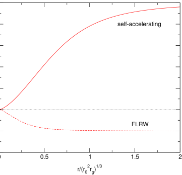
FIG. 1.: Mass discrepancy, $\delta M$, for a static point source whose Schwarzschild radius is $r_{g}$. The solid curve is for a self-accelerating background with $H=r_{0}^{-1}$. The dashed curve is for a FLRW background with $H=r_{0}^{-1}$.

The mass discrepancy between the lensing mass (the actual mass) and that determined from the Newtonian force may be read directly from Eqs. (37) and (39),

$$\delta M={M_{\rm lens}\over M_{\rm Newt}}-1={1\over 1+\delta(r)}-1\ .$$ (53)

This ratio is depicted in Fig. 1 for both cosmological phases. When the mass is measured deep within the Einstein regime, the mass discrepancy simplifies to

$$\delta M=\mp\left(r^{3}\over 2r_{0}^{2}R_{g}\right)^{1/3}\ .$$ (54)

Solar system measurements are too coarse to be able to resolve the DGP discrepancy between lensing mass of the sun and its Newtonian mass. The discrepancy $\delta M$ for the sun at ${\cal O}({\rm AU})$ scale distances is approximately $10^{-11}$. Limits on this discrepancy for the solar system as characterized by the post-Newtonian parameter, $\gamma-1$, are only constrained to be $<3\times 10^{-4}$.

A possibly more promising regime may be found in galaxy clusters. For $10^{14}\rightarrow 10^{15}~{}M_{\odot}$ clusters, the scale $(r_{0}^{2}R_{g})^{1/3}$ has the range $6\rightarrow 14~{}{\rm Mpc}$. For masses measured at the cluster virial radii of roughly $1\rightarrow 3~{}{\rm Mpc}$, this implies mass discrepancies of and taking their virial radii to be roughly $5\rightarrow 8\%$. X-ray or Sunyaev–Zeldovich (SZ) measurements are poised to map the Newtonian potential of the galaxy clusters, whereas weak lensing measurements can directly measure the cluster mass profile. Unfortunately, these measurements are far from achieving the desired precisions. If one can extend mass measurements to distances on the order of $r_{0}$, Fig. 1 suggests discrepancies can be as large as $-10\%$ for the FLRW phase or even $50\%$ for the self-accelerating phase.

C Orbit Precession

Imagine a body orbiting a mass source where $R_{g}(r)=r_{g}={\rm constant}$. The perihelion precession per orbit may be determined in the usual way

$$\Delta\phi=\int dr~{}{J\over r^{2}}{AN\over\sqrt{E^{2}-N^{2}\left(1+{J^{2}\over r^{2}}\right)}}\ ,$$ (55)

where $E=N^{2}dt/ds$ and $J=r^{2}d\phi/ds$ are again constants of motion resulting from the isometries, and now $ds$ is the differential proper time of the orbiting body. Assuming a nearly circular orbit and that we are deep within the Einstein regime (so that we may use Eqs. (41–42)), then

$$\Delta\phi=2\pi+{3\pi r_{g}\over r}\mp{3\pi\over 2}\left(r^{3}\over 2r_{0}^{2}r_{g}\right)^{1/2}\ .$$ (56)

The second term is the usual Einstein precession. The last term is the new anomalous precession due to DGP brane effects. Note that this correction is the same as one would get if one assumed a purely Newtonian potential Eq. (41) without spatial metric effects. The correction to the precession rate one expects from DGP gravity is

$${d\over dt}{\Delta\phi}_{\rm DGP}=\mp{3\over 8r_{0}}=\mp 5~{}\mu{\rm as/year}\ .$$ (57)

Note that this result is independent of the source mass, implying that this precession rate is a universal quantity dependent only on the graviton’s effective linewidth ($r_{0}^{-1}$) and the overall cosmological phase. Compare Eq. (57) to the classic Einstein precession correction for nearly circular orbits:

$${d\over dt}{\Delta\phi}_{\rm Einstein}={3\over 2}\left(r_{g}^{3}\over 2r^{5}\right)^{1/2}\ .$$ (58)

For increasing $r$, the distance from the sun at which the DGP correction begins to overtake the first Einstein correction is $37~{}{\rm AU}$.

Nordtvedt [20] quotes precision for perihelion precession at $430~{}\mu{\rm as/year}$ for Mercury and $10~{}\mu{\rm as/year}$ for Mars. Improvements in lunar ranging measurements [21, 22] suggest that the Moon will be sensitive to the DGP correction Eq. (57) in the near future. Also, BepiColombo, an ESA satellite being sent to Mercury at the end of the decade, will also be sensitive to this correction [23]. Incidentally, it is interesting to contrast these numbers with a precision of $4\times 10^{4}~{}\mu{\rm as/year}$ for the rate of periastron advance in Binary Pulsar PSR 1913+16 [24]. The solar system seems to provide the most promising means to constrain this anomalous precession from DGP gravity.

VI Concluding Remarks

The braneworld theory of Dvali–Gabadadze–Porrati (DGP) is an intriguing extension of Einstein gravity that exploits the possible existence of infinite-volume, extra dimensions. It is a theory where the four-dimensional graviton is effectively metastable, and provides a novel alternative to conventional explanations of the dark energy that is responsible for today’s cosmic acceleration.

In this paper, we detailed the solution of static, spherical matter sources in the background of deSitter cosmology for DGP gravity. The gravitational field of a matter source exhibits important dependences on cosmology. Residual dependences on the full five-dimensional cosmological phase also exist in the regime deep in the gravity well of the matter source where the effects of cosmology are ostensibly irrelevant. These residual dependences allow one to use local (e.g., solar system) measurements of the gravitational field to ascertain details of the global cosmology.

In DGP gravity, we find that massless test particles can probe the true mass of a matter source, whereas tests of the source’s Newtonian force leads to discrepancies with general relativity. These discrepancies translate into a universal anomalous precession, as large as $\pm 5~{}\mu{\rm as/year}$, suffered by all orbiting bodies. The numerical value of this anomalous precession is dependent only on the graviton’s effective linewidth and the global geometry of the five-dimensional cosmology. Current constraints on Mars’ orbit are on the threshold of being sensitive to this anomaly [20]. Future improvements in lunar ranging [22] as well as data from satellite missions at the end of the decade [23] should be sensitive to possible corrections due to DGP and gravitational leakage into extra dimensions.

In order to see why Eq. (27) is a reasonable approximation, we need to explore the full solution to the bulk Einstein equations,

$$G_{AB}(r,z)=0\ ,$$ (59)

satisfying the brane boundary conditions, Eqs. (16), as well as specifying that the metric approach the deSitter solution Eqs. (18–20) for large values of $r$ and $z$, i.e., far away from the compact matter source.

First, it is convenient to consider not only the components of the Einstein tensor Eqs. (11), but also the following components of the bulk Ricci tensor (which also vanishes in the bulk):

$$R_{t}^{t} = {1\over A^{2}}\left[{N^{\prime\prime}\over N}-{N^{\prime}\over N}{A^{\prime}\over A}+2{N^{\prime}\over N}{B^{\prime}\over B}\right]+\left[{\ddot{N}\over N}+{\dot{N}\over N}{\dot{A}\over A}+2{\dot{N}\over N}{\dot{B}\over B}\right]$$ (60)

$$R_{z}^{z} = {\ddot{N}\over N}+{\ddot{A}\over A}+{2\ddot{B}\over B}\ .$$ (61)

We wish to take $G_{zr}=0$, $G_{z}^{z}=0$, and $R_{z}^{z}=0$ and derive expressions for $A(r,z)$ and $B(r,z)$ in terms of $N(r,z)$. Only two of these three equations are independent, but it is useful to use all three to ascertain the desired expressions.

Since we are only interested in metric when $r,z\ll r_{0},H^{-1}$ for a weak matter source, we may rewrite the necessary field equations using the expressions Eqs. (25). Since the functions, $\{n(r,z),a(r,z),b(r,z)\}$ are small, we need only keep nonlinear terms that include $z$–derivatives. The brane boundary conditions, Eqs. (16), suggest that $\dot{a}$ and $\dot{b}$ terms may be sufficiently large to warrant inclusion of their subleading contributions. It is these $z$–derivative nonlinear terms that are crucial to the recover of Einstein gravity near the matter source. If one neglected these bilinear terms as well, one would revert to the linearized, weak-brane solution (cf. Ref. [13]).

Integrating Eq. (61) twice with respect to the $z$–coordinate, we get

$$n+a+2b=zg_{1}(r)+g_{2}(r)\ ,$$ (62)

where $g_{1}(r)$ and $g_{2}(r)$ are to be specified by the brane boundary conditions, Eqs. (16), and the residual gauge freedom $\delta b(r)|_{z=0}=0$, respectively. Integrating the $G_{zr}$–component of the bulk Einstein tensor Eqs. (11) with respect to the $z$–coordinate yields

$$r\left(n+2b\right)^{\prime}-2\left(a-b\right)=g_{3}(r)\ .$$ (63)

The functions $g_{1}(r)$, $g_{2}(r)$, and $g_{3}(r)$ are not all independent, and one can ascertain their relationship with one another by substituting Eqs. (62) and (63) into the $G_{z}^{z}$ bulk equation. If one can approximate $\dot{n}=\mp H$ for all $z$, then one can see that $G_{zr}=0$, $G_{z}^{z}=0$, and $R_{z}^{z}=0$ are all consistently satisfied by Eqs. (62) and (63), where the functions $g_{1}(r)$, $g_{2}(r)$, and $g_{3}(r)$ are determined at the brane using Eqs. (37) and (38) and the residual gauge freedom $b(r)|_{z=0}=0$:

$$g_{1}(r) = \mp 4H-{r_{0}\over r^{2}}\left(R_{g}\delta\right)^{\prime}$$ (64)

$$g_{2}(r) = {R_{g}\over 2r}(1-\delta)+\int_{0}^{r}dr~{}{R_{g}\over r^{2}}(1+\delta)$$ (65)

$$g_{3}(r) = {R_{g}\over 2r}(1-3\delta)-2H^{2}r^{2}\ ,$$ (66)

where we have used the function $\delta(r)$, defined in Eq. (39). Using Eqs. (62–66), we now have expressions for $a(r,z)$ and $b(r,z)$ completely in terms of $n(r,z)$ for all $(r,z)$.

Now we wish to find $n(r,z)$ and to confirm that $\dot{n}=\mp H$ is a good approximation everywhere of interest. Equation (60) becomes

$$n^{\prime\prime}+{2n^{\prime}\over r}+\ddot{n}=\pm H[g_{1}(r)\pm H]\ ,$$ (67)

where again we have neglected contributions if we are only concerned with $r,z\ll r_{0},H^{-1}$. Using the expression Eq. (64), we find

$$n^{\prime\prime}+{2n^{\prime}\over r}+\ddot{n}=-3H^{2}\mp{r_{0}H\over r^{2}}\left[R_{g}\delta(r)\right]^{\prime}\ .$$ (68)

Then, if we let

$$n=1\mp Hz-{1\over 2}H^{2}r^{2}\mp r_{0}H\int_{0}^{r}dr~{}{1\over r^{2}}R_{g}(r)\delta(r)+\delta n(r,z)\ ,$$ (69)

where $\delta n(r,z)$ satisfies the equation

$$\delta n^{\prime\prime}+{2\delta n^{\prime}\over r}+\ddot{\delta n}=0\ ,$$ (70)

we can solve Eq. (70) by requiring that $\delta n$ vanish as $r,z\rightarrow\infty$ and applying the condition

$$r~{}\delta n^{\prime}|_{z=0}={R_{g}\over 2r}\left[1+(1\pm 2r_{0}H)\delta(r)\right]\ ,$$ (71)

on the brane as an alternative to the appropriate brane boundary condition for $\delta n(r,z)$ coming from a linear combination of Eqs. (16). We can write the solution explicitly:

$$\delta n(r,z)=\int_{0}^{\infty}dk~{}c(k)e^{-kz}\sin kr\ ,$$ (72)

where

$$c(k)={2\over\pi}\int_{0}^{\infty}dr~{}r\sin kr\left.\delta n\right|_{z=0}(r)\ .$$ (73)

We can then compute $\dot{\delta n}|_{z=0}$, arriving at the bound

$$\dot{\delta n}|_{z=0}\lesssim{1\over r}\int_{0}^{r}dr~{}{R_{g}(r)\over r^{2}}\ ,$$ (74)

for all $r\ll r_{0},H^{-1}$. Then,

$$\dot{n}|_{z=0}=\mp H+\dot{\delta n}|_{z=0}\ .$$ (75)

When the first term in Eq. (75) is much larger than the second, Eq. (27) is a good approximation. When the two terms in Eq. (75) are comparable or when the second term is much larger than the first, neither term is important in the determination of Eqs. (37) and (38). Thus, Eq. (27) is still a safe approximation.

One can confirm that all the components of the five-dimensional Einstein tensor, Eqs. (11), vanish in the bulk using field variables satisfying the relationships Eqs. (62), (63), and (69). The field variables $a(r,z)$ and $b(r,z)$ both have terms that grow with $z$, stemming from the presence of the matter source. However, one can see that with the following redefinition of coordinates:

$$R = r-zr_{0}{R_{g}\delta\over r^{2}}$$ (76)

$$Z = z+\int_{0}^{r}dr~{}{R_{g}\delta\over r^{2}}\ ,$$ (77)

that to leading order as $z\rightarrow H^{-1}$, the desired $Z$–dependence is recovered for $a(R,Z)$ and $b(R,Z)$ (i.e., $\mp HZ$), and the Newtonian potential takes the form

$$n(R,Z)=\mp HZ-{1\over 2}H^{2}R^{2}+\cdots\ .$$ (78)

Thus, we recover the desired asymptotic form for the metric of a static, compact matter source in the background of a deSitter expansion.

REFERENCES

- [1] G. Dvali, G. Gabadadze and M. Porrati, Phys. Lett. B 485, 208 (2000).
- [2] G. R. Dvali, G. Gabadadze, M. Kolanovic and F. Nitti, Phys. Rev. D 64, 084004 (2001).
- [3] G. R. Dvali, G. Gabadadze, M. Kolanovic and F. Nitti, Phys. Rev. D 65, 024031 (2002).
- [4] C. Deffayet, Phys. Lett. B 502, 199 (2001).
- [5] C. Deffayet, G. R. Dvali and G. Gabadadze, Phys. Rev. D 65, 044023 (2002).
- [6] C. Deffayet, S. J. Landau, J. Raux, M. Zaldarriaga and P. Astier, Phys. Rev. D 66, 024019 (2002).
- [7] J. S. Alcaniz, Phys. Rev. D 65, 123514 (2002).
- [8] D. Jain, A. Dev and J. S. Alcaniz, Phys. Rev. D 66, 083511 (2002).
- [9] J. S. Alcaniz, D. Jain and A. Dev, Phys. Rev. D 66, 067301 (2002).
- [10] A. Lue, arXiv:hep-th/0208169.
- [11] C. Deffayet, G. R. Dvali, G. Gabadadze and A. I. Vainshtein, Phys. Rev. D 65, 044026 (2002).
- [12] A. Lue, Phys. Rev. D 66, 043509 (2002).
- [13] A. Gruzinov, arXiv:astro-ph/0112246.
- [14] M. Porrati, Phys. Lett. B 534, 209 (2002).
- [15] C. Middleton and G. Siopsis, arXiv:hep-th/0210033.
- [16] G. Kofinas, E. Papantonopoulos and I. Pappa, arXiv:hep-th/0112019.
- [17] G. Kofinas, E. Papantonopoulos and V. Zamarias, arXiv:hep-th/0208207.
- [18] C. Deffayet, arXiv:hep-th/0205084.
- [19] C. Deffayet, talk given at “Peyresq Physics 7” Conference, June 2002, Peyresq (France).
- [20] K. Nordtvedt, Phys. Rev. D 61, 122001 (2000).
- [21] J. G. Williams, X. X. Newhall and J. O. Dickey, Phys. Rev. D 53, 6730 (1996).
- [22] G. Dvali, A. Gruzinov, and M. Zaldarriaga, hep-ph/0212069.
- [23] A. Milani, D. Vokrouhlicky, D. Villani, C. Bonanno and A. Rossi, Phys. Rev. D 66, 082001 (2002).
- [24] C. M. Will, Living Rev. Rel. 4, 4 (2001) [arXiv:gr-qc/0103036].