Cosmological constraints from evolution of
cluster baryon mass function at $z\sim 0.5$

Abstract

We present a new method for deriving cosmological constraints based on the evolution of the baryon mass function of galaxy clusters, and implement it using 17 distant clusters from our 160 deg² ROSAT survey. The method uses the cluster baryon mass as a proxy for the total mass, thereby avoiding the large uncertainties of the $M_{\text{tot}}-T$ or $M_{\text{tot}}-L_{X}$ relations used in all previous studies. Instead, we rely on a well-founded assumption that the $M_{b}/M_{\text{tot}}$ ratio is a universal quantity, which should result in a much smaller systematic uncertainty. Taking advantage of direct and accurate Chandra measurements of the gas masses for distant clusters, we find strong evolution of the baryon mass function between $z>0.4$ and the present. The observed evolution defines a narrow band in the $\Omega_{m}-\Lambda$ plane, $\Omega_{m}+0.23\Lambda=0.41\pm 0.10$ at 68% confidence, which intersects with constraints from the Cosmic Microwave Background and supernovae Ia near $\Omega_{m}=0.3$ and $\Lambda=0.7$.

1. Introduction

The growth of large scale structure in the near cosmological past is very sensitive to the value of the density parameter, $\Omega_{m}$, and, weakly, to the cosmological constant, $\Lambda$ (see, among others, Sunyaev 1971, Peebles 1980, Carroll, Press & Turner 1992). One of the strongest manifestations of the growth of density perturbations is the formation of virialized objects such as clusters of galaxies (Press & Schechter 1974). Therefore, the evolution of the cluster mass function provides a sensitive cosmological test (e.g. Evrard 1989 and later works).

Present-day theory provides machinery for accurate predictions for the cluster mass function at any redshift, in any cosmology (see a brief review in § 4). Most of the difficulties with using cluster evolution as a cosmological probe are on the observational side. The foremost problem is the necessity to relate cluster masses with other observables, such as the X-ray temperature. Even for the few brightest, best-studied clusters, the total mass within the virial radius — the quantity generally used in theory — is measured presently with large uncertainties (see, e.g., Markevitch & Vikhlinin 1997 and Fischer & Tyson 1997 for representative uncertainty estimates for the X-ray hydrostatic and weak lensing methods, respectively). To measure virial masses in a large, complete sample of clusters is presently impractical. Therefore, one usually resorts to other, more easily measurable quantities, which exhibit scaling relations with the total mass. The most widely used observable is the temperature of the intracluster medium. It is expected that $T$ is related to the virial mass as $M\propto T^{3/2}$, and the available observations generally support this law (Nevalainen, Markevitch & Forman 2000; Horner, Mushotzky & Scharf 1999; Finoguenov, Reiprich & Böhringer 2001). To normalize this relation, virial masses still have to be measured in a representative sample of clusters. Any systematic uncertainties in the cluster mass measurements translate into the same uncertainty in the normalization of the $M-T$ relation.

The X-ray temperature functions (XTF) for both nearby and distant clusters have been used as a proxy for the mass function by a number of authors, using the normalization of the $M-T$ relation from different sources. An analysis of a statistically complete local XTF was first performed by Henry & Arnaud (1991). The analysis of the local XTF yields the normalization ($\sigma_{8}$), in combination with $\Omega_{m}$, and slope of the power spectrum of density fluctuations on cluster scales. This type of study has since been applied to ever improving observational data (see Evrard et al. 2002 for a recent summary).

A first cosmological measurement using the evolution of the XTF at redshifts greater than zero is due to Henry (1997), who derived $\Omega_{m}\approx 0.5\pm 0.15$. A similar analysis was performed by Eke et al. (1998), Donahue & Voit (1999), Henry (2000), Blanchard et al. (2000), with updates on both observational and theoretical sides as well as with different normalizations of the $M-T$ relation. We also note the studies by Reichart et al. (1999) and Borgani et al. (2001) who modeled the X-ray luminosity functions for distant clusters using an empirical $L-T$ relation and the usual theory for the XTF evolution.

Theoretical prediction for the number density of clusters with a given temperature is exponentially sensitive to the normalization of the $M-T$ relation. A 30% change in the normalization of the $M-T$ relation results in a 20% change in the determination of the $\sigma_{8}$ parameter and shifts an estimate of $\Omega_{m}$ by a factor of 1.3–1.4 (e.g., Rosati, Borgani & Norman 2002). Given that $\pm 50\%$ is a fair estimate of the present systematic uncertainties in the $M-T$ normalization, the impact of this relation on cosmological parameter determination can be very significant.

In modeling the high-redshift temperature function, the theoretically expected evolution of the $M-T$ relation is usually assumed: $M\propto T^{3/2}/(1+z)^{3/2}$. It would be very important to verify this evolution at high $z$. Unfortunately, this seems to push the limits of current observational techniques. The evolution of other scaling relations can be also quite important. For example, the $L-T$ relation is required for computing the volume of X-ray flux limited surveys, and for estimating cluster masses, when the X-ray luminosity function is used as a proxy for the mass function. Most of the previous studies have assumed that the $L-T$ relation does not evolve, however recent Chandra measurements indicate otherwise (Vikhlinin et al. 2002).

Finally, most of the available cosmological studies are based on the distant cluster sample from the Einstein Extended Medium Sensitivity Survey (Gioia et al. 1990, Henry et al. 1992). The completeness of this survey at high redshifts is often questioned (Nichol et al. 1997; Ebeling et al. 2000; Lewis et al. 2002). Although we believe that the EMSS is essentially complete (as confirmed by good agreement between the XLFs from the EMSS and several ROSAT surveys — Gioia et al. 2001, Vikhlinin et al. 2000, Mullis et al., in preparation), it is arguably important to try another completely independent sample for the cosmological studies based on cluster evolution.

The purpose of this paper is to apply the evolutionary test to a new sample of distant, $z>0.4$, clusters derived from the 160 deg² ROSAT survey (Vikhlinin et al. 1998), relying on the evolution of the cluster scaling relations as measured by Chandra, and using a modeling technique which does not rely upon the total mass measurements to normalize the $M-T$ or $M-L$ relations and therefore bypasses many of the uncertainties mentioned above.

The proposed method relies on the assumption that the baryon fraction within the virial radius in clusters should be close to the average value in the Universe, $f_{b,U}=\Omega_{b}/\Omega_{m}$. This is expected on general theoretical grounds (White et al. 1993) because gravity is the dominant force on cluster scales. The universality of the baryon fraction in massive clusters is supported by cosmological numerical simulations (e.g. Bialek, Evrard & Mohr 2001) and by most available observations (most recently, Allen et al. 2002). In principle, the equality $f_{b}=\Omega_{b}/\Omega_{m}$ can be used to determine cosmological parameters either from the absolute measurements of $f_{b}$ in the nearby clusters (White et al. 1993) or from the apparent redshift dependence of $f_{b}$ measurements in the high-redshift clusters (Sasaki 1996, Pen 1997). Both methods, however, require an accurate observational determination of the total mass in individual clusters, which we would like to avoid.

Unlike the total mass, the baryon mass in clusters is relatively easily measured to the virial radius (Vikhlinin et al. 1999). To first order, the baryon and total mass are trivially related, $M_{b}=M\,\Omega_{b}/\Omega_{m}.$ If this is the case, the relation between the cumulative total mass function, $F(M)$, and the baryon mass function, $F_{b}(M_{b})$, is also trivial,

$$F_{b}(M_{b})=F\left(\Omega_{m}/\Omega_{b}\,M_{b}\right).$$ (1)

The average baryon density in the Universe is accurately given by observations of the light element abundances and Big Bang Nucleosynthesis theory (Burles, Nollet & Turner 2001). Therefore, we have everything needed to convert the theoretical model for the total mass function, $F(M)$, to the prediction for a directly measurable baryon mass function — to compute $F(M)$ one must choose a value of $\Omega_{m}$, which fixes the scaling between the total and baryon mass. The conversion of the total to the baryon mass function — at least to a first approximation — can be expressed through the model parameters, and therefore $F_{b}(M_{b})$ can be modeled with the usual set of parameters, $\Omega_{m}$, $\sigma_{8}$, $n$, $h$, and at a high redshift — $\Lambda$. We will show below that the evolution of the baryon mass function provides robust constraints on a combination of $\Omega_{m}$ and $\Lambda$. Modeling of the baryon mass function at $z=0$ provides a measurement of the power spectrum normalization, $\sigma_{8}$, and of the shape parameter $\Gamma=\Omega_{m}\,h$, with degeneracies that differ from those given by the temperature function (Voevodkin & Vikhlinin, in preparation).

Theoretical models of the cluster mass function usually consider masses measured within radii defined by certain values of the density contrast, $\delta=3M(r)/(4\pi\,r^{3})/\rho$, where $\rho$ is either the critical density or mean density of the Universe. The assumption that the baryon fraction in clusters is universal at sufficiently large radii allows one to determine the overdensity radii $r_{\delta}$ without measuring the total mass. Indeed, the baryon and matter overdensities are then equal, $\delta_{b}=\delta$, and the baryon overdensity is defined by a baryon mass $M_{b}(r)$ and the mean baryon density in the Universe, known from the BBN. One of the most accurate theoretical models for the mass function (Jenkins et al. 2001) uses masses corresponding to the overdensity $\delta=324$ relative to the mean density of the Universe at the redshift of observation. The matching baryon masses, $M_{b,324}$ are easily measured using ROSAT data for nearby clusters (Voevodkin, Vikhlinin & Pavlinsky 2002a, VVPa hereafter), and Chandra data for distant clusters (Vikhlinin et al. 2002).

The paper is organized as follows. In § 2, we discuss the distant cluster sample and the gas mass measurements in the distant and nearby clusters. The baryon mass function for distant clusters is derived in § 3. The theory for modeling these data is reviewed in § 4. We describe our fitting procedure in § 5, and present the derived constraints on $\Omega_{m}$ and $\Lambda$ in § 6.

All cluster parameters are quoted for $h=0.65$, $\Omega_{m}=0.3$, and $\Lambda=0.7$. The X-ray fluxes and luminosities are in the 0.5–2 keV energy band. Measurement uncertainties are $1\sigma$.

2. Data

Table 1X-ray data and baryon masses for the distant 160 deg² clusters

Cluster $z$ $f_{0.5-2}$ (ROSAT) $L_{0.5-2}$ $M_{g,324}$ $M_{b,324}$ $f_{0.5-2}$ (Chandra) (erg s^-1 cm^-2) (erg s^-1) $(10^{13}\,M_{\odot})$ $(10^{13}\,M_{\odot})$ (erg s^-1) CL 1416+4446 0.400 $4.04\times 10^{-13}$ $2.5\times 10^{44}$ $8.0\pm 2.3$ $9.8\pm 2.8$ $4.51\times 10^{-13}$ CL 1701+6414 0.453 $3.86\times 10^{-13}$ $2.9\times 10^{44}$ $10.4\pm 2.8$1 $12.5\pm 3.4$1 $4.14\times 10^{-13}$ CL 1524+0957 0.516 $3.04\times 10^{-13}$ $2.7\times 10^{44}$ $9.3\pm 2.3$ $11.2\pm 2.8$1 $2.81\times 10^{-13}$ CL 1641+4001 0.464 $2.94\times 10^{-13}$ $2.3\times 10^{44}$  $\cdots$ $8.3\pm 2.9$  $\cdots$ CL 0030+2618 0.500 $2.43\times 10^{-13}$ $2.3\times 10^{44}$ $6.6\pm 2.7$ $8.1\pm 3.3$ $2.51\times 10^{-13}$ CL 1120+2326 0.562 $2.13\times 10^{-13}$ $2.2\times 10^{44}$ $6.6\pm 1.5$ $8.2\pm 1.9$ $1.88\times 10^{-13}$ CL 1221+4918 0.700 $2.06\times 10^{-13}$ $4.1\times 10^{44}$ $11.3\pm 2.1$1 $13.6\pm 2.6$1 $2.25\times 10^{-13}$ CL 0853+5759 0.475 $1.98\times 10^{-13}$ $1.6\times 10^{44}$  $\cdots$ $6.3\pm 2.2$  $\cdots$ CL 0522–3625 0.472 $1.84\times 10^{-13}$ $1.5\times 10^{44}$  $\cdots$ $5.9\pm 2.1$  $\cdots$ CL 1500+2244 0.450 $1.78\times 10^{-13}$ $1.3\times 10^{44}$  $\cdots$ $5.5\pm 1.9$  $\cdots$ CL 0521–2530 0.581 $1.76\times 10^{-13}$ $2.3\times 10^{44}$  $\cdots$ $7.2\pm 2.5$  $\cdots$ CL 0926+1242 0.489 $1.67\times 10^{-13}$ $1.5\times 10^{44}$  $\cdots$ $5.7\pm 2.0$  $\cdots$ CL 0956+4107 0.587 $1.56\times 10^{-13}$ $2.0\times 10^{44}$  $\cdots$ $6.6\pm 2.3$  $\cdots$ CL 1216+2633 0.428 $1.54\times 10^{-13}$ $1.0\times 10^{44}$  $\cdots$ $4.6\pm 1.6$  $\cdots$ CL 1354–0221 0.546 $1.45\times 10^{-13}$ $1.6\times 10^{44}$  $\cdots$ $5.8\pm 2.0$  $\cdots$ CL 1117+1744 0.548 $1.44\times 10^{-13}$ $1.6\times 10^{44}$  $\cdots$ $5.8\pm 2.0$  $\cdots$ CL 1213+0253 0.409 $1.43\times 10^{-13}$ $0.9\times 10^{44}$  $\cdots$ $4.2\pm 1.5$  $\cdots$

All distance-dependent quantities are derived assuming $\Omega_{m}=0.3$, $\Lambda=0.7$, and $h=0.65$. For different values of the Hubble constant, masses scale as $h^{-2.25}$. The luminosities are determined using the ROSAT fluxes, not the Chandra measurements. The baryon mass (i. e. gas+stars) is estimated from the gas mass using (2). For CL 1641+4001 and all clusters with $f<2\times 10^{-13}$ erg s^-1 cm^-2, the values of $M_{b,324}$ are estimated from the $L-M_{b}$ relation.

2.1. Distant Cluster Sample

The sample of distant clusters used in this work is derived from our 160 deg² survey (Vikhlinin et al. 1998). This survey is based on the X-ray detection of serendipitous clusters in the central parts of a large number of the ROSAT PSPC observations. The spatial extent of the X-ray sources is used as a primary selection criterion, but it is verified by independent surveys (Perlman et al. 2002) that above the advertised flux limits, we do not miss any clusters because of the limited angular resolution of ROSAT. Therefore, for all practical purposes the 160 deg² cluster sample can be considered as flux-limited.

The optical identification of the entire X-ray sample is now complete and redshifts of all clusters are spectroscopically measured (Mullis et al., in preparation). Optical identifications show that our X-ray selection is very efficient. In the entire sample, only 20 of the 223 detected X-ray cluster candidates lack a cluster identification. Above the median flux of the survey, $f>1.4\times 10^{-13}$ erg s^-1 cm^-2, 111 of 114 sources (or 98%) were confirmed as clusters. Therefore, the 160 deg² survey is in effect purely X-ray selected.

Our X-ray detection procedure is fully automatic, and therefore all essential statistical characteristics of the survey can be derived from Monte-Carlo simulations. We have performed very extensive simulations to calibrate the process of detection of clusters with different fluxes and radii. This gave an accurate determination of the survey sky coverage as a function of flux (Vikhlinin et al. 1998), and therefore of the survey volume for any combination of cosmological parameters.

2.2. Chandra Observations

As of Fall 2002, Chandra has observed 6 clusters from the 160 deg² sample. These objects almost complete a flux-limited subsample, $f>2\times 10^{-13}$ erg s^-1 cm^-2, of objects at $z>0.4$ (7 total), and therefore they are suitable for statistical studies. Chandra observations of these clusters are discussed in Vikhlinin et al. (2002). Briefly, the quality of the X-ray data allows a measurement of the cluster temperature to a 10% accuracy, and of the gas mass at the virial radii with a $20\%$ uncertainty. For the purposes of this paper, we need only the measurements of the gas mass.

The Chandra observations of the distant 160 deg² clusters as well as those from the EMSS and RDCS (Rosati et al. 1998) samples show that scaling relations between the X-ray luminosity, temperature, and the gas mass significantly evolve with redshift (Vikhlinin et al. 2002). In particular, the $L-M_{g}$ relation evolves so that the gas mass for a fixed luminosity is proportional to $(1+z)^{-1.8\pm 0.25}$ but the slope and scatter in the high-redshift relation are the same as in the local relation (Voevodkin, Vikhlinin & Pavlinsky 2002b, VVPb hereafter). This allows an estimate of the gas mass, with a $\pm 35\%$ uncertainty, from the easily measured X-ray flux.

The $L-M_{g}$ relation allows us to extend the estimate of the gas mass to all high-redshift clusters that do not have Chandra observations. However, we will use only clusters with $f>1.4\times 10^{-13}$ erg s^-1 cm^-2. At $z=0.4$, this flux limit corresponds roughly to $T=3$ keV. It is possible that for much less massive clusters, our basic assumption of the universality of the baryon fraction may not hold due to, e. g., preheating of the intracluster medium (e.g., Bialek et al. 2001). The median redshift for the selected distant clusters is $z=0.55$.

The measurements and estimates of the baryon mass in distant clusters are listed in Table 1. The measured masses were derived using direct deprojection of the X-ray surface brightness profiles. The mass uncertainties were obtained by error propagation in the process of deprojection and so correctly reflect the statistical noise in the surface brightness profiles near $r_{324}$. The only object with Chandra data which was not used by Vikhlinin et al. (2002), is CL 0030+2618. This cluster was observed very soon after the Chandra launch while the detector parameters did not yet reach their nominal values. These data are unusable for spectral (temperature) measurements, but the imaging analysis which yields the gas mass can be performed without any complications.

The baryon masses were estimated from the $M_{b}-L$ correlation for approximately 60% of clusters in our distant sample. Both quantities in the $M_{b}-L$ correlation are easily and directly measured, and so there is no systematic uncertainty in the derivation of normalization, or slope, or evolution of this relation.

Finally, we remark on the excellent agreement of the X-ray fluxes for the 160 deg² survey clusters derived from ROSAT and Chandra data. For the 6 clusters in common, the ROSAT fluxes deviate by no more than 13%, always within the statistical uncertainties. The average ratio of the ROSAT and Chandra fluxes is $0.99\pm 0.06$.

2.3. Summary of the Low-Redshift Results

The baryon mass measurements in a large sample of low-redshift clusters, as well as the determination of the baryon mass function at $z=0.05$ was reported in VVPa,b. These results provide a low-redshift reference point for our measurement of cluster evolution, so a brief summary is in order.

VVP have used a flux-limited subsample of the low-redshift clusters detected in the ROSAT All-Sky Survey. The initial object selection was performed using the HIFLUGCS sample (Reiprich & Böhringer 2001). The X-ray fluxes were re-measured and 52 clusters were selected in the redshift interval $0.01<z<0.25$ and with $f_{x}>1.4\times 10^{-11}$ erg s^-1 cm^-2. The median redshift of this sample is $z=0.05$. Most of these clusters have ROSAT PSPC pointed observations which were used to measure the gas mass (the procedure is described in VVPa and Vikhlinin, Forman & Jones 1999).

Using a subsample of clusters with published optical measurements, a tight correlation between the gas mass and optical luminosity of the cluster has been established. This relation allows an estimate of the baryon (i. e. gas+galaxies but excluding intergalactic stars) mass of all clusters from the X-ray data alone:

$$M_{b,324}=M_{g,324}\times\left[1.100+0.045\left(\frac{M_{g,324}}{10^{15}\,M_{\sun}}\right)^{-0.5}\right],$$ (2)

where $M_{b,324}$ is the baryon mass corresponding to the overdensity $\delta=324$, and $M_{g,324}$ is the gas mass corresponding to $\delta=324$ without accounting for the stellar mass. The stellar contribution to the baryon mass is small, but non-negligible, of order 10–15% for massive clusters (this is consistent with the estimates in Fukugita, Hogan & Peebles 1998). This is estimated with approximately 25% uncertainty (i. e. $\pm 3\%$ of the total baryon mass). Assuming that the ratio of stellar and gas mass does not evolve at high $z$, i. e. that the galaxies neither confine the intracluster gas nor lose their mass significantly due to stellar winds, equation (2) can be used to estimate the baryon mass in distant clusters (our results are not sensitive to this assumption).

VVPb have derived the low-redshift baryon mass function (reproduced below). The measurement uncertainties in this mass function were determined using a technique which accounts for the Poisson noise as well as the individual $M_{b}$ measurement uncertainties (see also Appendix).

Figure 1.— Left: Comoving volume of the 160 deg² survey for $0.4<z<0.8$ as a function of the cluster baryon mass. Right: Volume per unit redshift interval for three values of $M_{b}$ — 0.25, 0.5, and $1\times 10^{14}\,M_{\sun}$ (from bottom to top). On each panel, the solid lines are for the $\Omega_{m}=0.3$, $\Lambda=0.7$ cosmology, and dashed lines are for $\Omega_{m}=1$, $\Lambda=0$. The volumes are computed for a limiting X-ray flux of $f_{\text{min}}=1.4\times 10^{-13}$ erg s^-1 cm^-2.

To summarize, the baryon mass function for the low-redshift clusters is measured reliably. By itself, it provides constraints on the shape and normalization of the power spectrum of the density perturbations, i.e. on the parameters $\sigma_{8}$ and $\Gamma=\Omega_{m}\,h$. These results will be reported in Voevodkin & Vikhlinin (in preparation). In the present Paper, we restrict ourselves to the cosmological constraints derived from the evolution of the mass function between $z>0.4$ and $z\simeq 0$.

3. Baryon mass function at $z>0.4$

In this section, we use the Chandra observations to derive the baryon mass function for distant clusters. First, we describe the computations of the survey volume as a function of mass.

3.1. Survey Volume

We consider the mass function for $0.4\leq z\leq 0.8$. Since our cluster sample is selected by X-ray flux, the computation of the surveyed volume as a function of mass is only possible if there is a correlation between the baryon mass and X-ray luminosity. Such a correlation is observed (VVPb, Vikhlinin et al. 2002),

$$M_{b}\propto(1+z)^{A_{ML}}L_{X}^{0.83}$$ (3)

with a 42% scatter in luminosity and 35% scatter in mass; $L_{X}$ is the total luminosity in the 0.5–2 keV band.

In the case of zero scatter in the $M_{b}-L$ relation, the volume is computed as

$$V=\int_{z_{\text{min}}}^{z_{\text{max}}}A(f)\;\frac{dV}{dz}\;dz,\;\;f=\frac{C\,M_{b}^{1.20}(1+z)^{-1.20A_{ML}}\,S(z)}{4\pi\,d_{L}^{2}(z)}$$ (4)

where $A(f)$ is the survey area as a function of flux, $dV/dz$ is the cosmological dependence of the comoving volume, equation (3) is rewritten as $L=C\,M^{1.20}(1+z)^{-1.20A_{ML}}$, and $S(z)$ is a correction for redshifting of the bandpass (equivalent to the K-correction in the optical astronomy). Note that for the non-evolving $L-T$ relation, $S(z)$ is independent of cosmology. The corrections due to the observed rate of evolution in this relation (Vikhlinin et al. 2002) are small, $\sim 5\%$ in volume, and they were ignored.

Introducing the scatter in the $M_{b}-L$ relation with the log-normal distribution (see VVPb), equation (4) becomes

$$\begin{split}V=&\frac{1}{(2\pi)^{1/2}\sigma}\int_{z_{\text{min}}}^{z_{\text{max}}}\int_{-\infty}^{\infty}\exp\left(-\lg^{2}y/2\sigma^{2}\right)\,d\lg y\;\times\\ &\;\;\;\times A\left(y\;\frac{C\,M^{1.20}(1+z)^{-1.20A_{ML}}\,S(z)}{4\pi\,d_{L}^{2}(z)}\right)\;\frac{dV}{dz}\;dz,\end{split}$$ (5)

where $\sigma=0.173$ is the observed rms log-scatter in the local mean $M_{b}-L$ relation (VVPb). Numerical integration of this equation gives the survey volume as a function of baryon mass for any set of the cosmological parameters $\Omega_{m}$, $\Lambda$, and $h$. The inner integral in (5) represents the effective value of the survey volume per unit redshift interval for clusters of given mass, $(dV/dz)_{\text{eff}}$.

There is no simple scaling of $V(M)$ with either $\Omega_{m}$ or $\Lambda$. In addition to $dV/dz$, the index $A_{ML}$ is also cosmology-dependent. When fitting the mass function to different cosmological models, we recomputed $V(M)$ for every new combination of the model parameters.

Figure 1 shows the comoving volume in the redshift interval $0.4<z<0.8$ as a function of the baryon mass. Note that in the limit of large masses, the survey volume approaches that of the local all-sky surveys.

The right panel of Fig. 1 shows a volume per unit redshift interval for three values of $M_{b}$. The clusters with small masses generally have low luminosities and therefore can be detected only near the lower boundary of the redshift interval considered. Massive clusters can be detected at any $z$, and therefore most of the volume for such clusters is accumulated near the higher boundary. This dependence of $(dV/dz)_{\text{eff}}$ on mass should be taken into account in modeling the mass function because the evolutionary effects between $z=0.4$ and $0.8$ are quite strong.

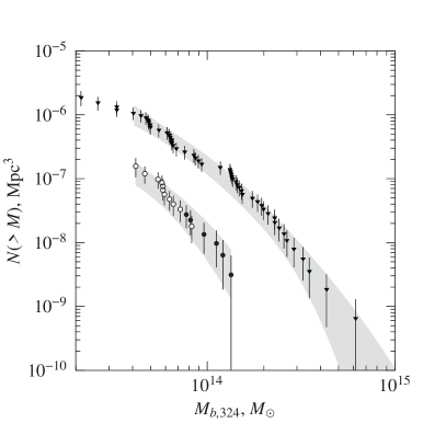
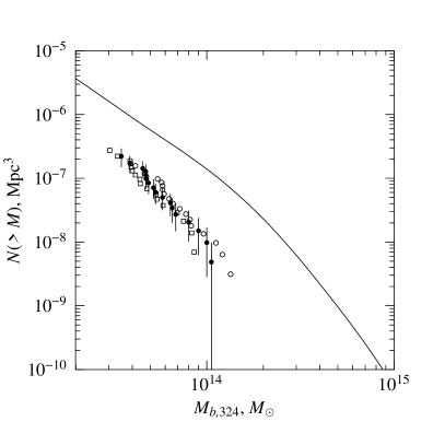
Figure 2.— Left: The baryon mass function for the 160 deg² survey sample in the redshift interval $0.4<z<0.8$. The local mass function from Voevodkin et al. (2002b) is shown by triangles. The grey band shows a 68% uncertainty interval for the mass functions, including both the Poisson noise and mass measurement uncertainties. The mass function at $z>0.4$ is shown by circles. The solid circles correspond to clusters with Chandra baryon mass measurements, and the empty circles to the mass estimates from the $M_{b}-L$ relation. The high-redshift mass function is computed for $\Omega_{m}=0.3$, $\Lambda=0.7$; the local mass function is cosmology-independent. Right: Baryon mass functions derived assuming $\Omega_{m}=0.3$, $\Lambda=0.7$ (empty circles); $\Omega_{m}=0.3$, $\Lambda=0$ (solid circles); $\Omega_{m}=1$, $\Lambda=0$ (squares). The solid line shows a fit to the local mass function. On both panels, the data are for $h=0.5$. The measured $M_{b}$ scales as $M_{b}\propto h^{-2.25}$ and volume scales as usual, $V\propto h^{-3}$

3.2. Observed Baryon Mass Function

Since the number of clusters in our sample is rather small, we will work with the integral representation of the mass function, which is determined as

$$F(M)=N(>M)=\sum_{M_{b}^{(i)}>M}\frac{1}{V(M_{b}^{(i)})},$$ (6)

The Poisson errorbars for $F(M)$ are computed as

$$(\Delta F)^{2}=\sum_{M_{b}^{(i)}>M}\frac{1}{V^{2}(M_{b}^{(i)})}.$$ (7)

In addition to the Poisson noise, the $F(M)$ errorbars should include an additional component reflecting the individual mass measurement uncertainties. This was done using the Maximum Likelihood analysis described in the Appendix. We estimate that other obvious sources of uncertainty in $F(M)$ are small. For example, the inaccuracies of the survey volume caused by uncertainties in the 160 deg² sky coverage or variations of the evolution or scatter in the $M_{b}-L$ relation within the observationally allowed intervals are all below 10%, which is much smaller than the Poisson noise in the mass function, so we ignore them.

The baryon mass function computed in the $\Omega_{m}=0.3$, $\Lambda=0.7$ cosmology is shown in Fig. 2. A comparison with the local $F(M)$ from VVPb shows a strong evolution — at $z\approx 0.5$ there are approximately 10 times fewer clusters of the same mass per unit comoving volume than at $z=0$. This evolution is quite insensitive to the assumed cosmology. The right panel in Fig. 2 shows the mass functions computed assuming several combinations of $\Omega_{m}$ and $\Lambda$. Mostly, the changes are restricted to a translation along the band defined by $F(M)$ itself.

Part of the evolution of the mass function in Fig. 2 may be unrelated to the physical growth of clusters and instead related to the commonly used definition of mass. Indeed, let us assume that all clusters stay exactly the same at all redshifts. The operational definition of mass used in our study is related to the density contrast above the mean density of the Universe at the cluster redshift. Since the mean density changes as $(1+z)^{3}$, the radius of the fixed contrast decreases with redshift, and therefore the mass also decreases. For the average density profile at large radii, we find that this effect results in the mass scaling $M\sim(1+z)^{-1.5}$. This mass offset explains about 40% of the observed effect, and the rest is due to the real growth, by a factor of $\sim 2$ in mass, of clusters between $z>0.4$ and $z=0$.

As was explained above, the total mass functions are related to the baryon mass functions through a constant log shift along the mass axis, which does not alter the vertical offset between the local and high-redshift functions. The vertical offset is related to the growth of density fluctuations between $z>0.4$ and $z=0$. Below, we use it to derive constraints on the parameters $\Omega_{m}$ and $\Lambda$.

4. Theory

Our computations of the theoretical mass functions are based on the Jenkins et al. (2001) universal fit to the mass functions in large-volume cosmological simulations. Jenkins et al. find that the mass functions expressed in terms of the rms density fluctuations on mass scale $M$ are of a universal form:

$$f(\sigma)=-\frac{M}{\langle\rho\rangle}\,\frac{d\,n(M)}{d\ln\sigma^{-1}}=A\,\exp\left(-|\ln\sigma^{-1}+b\,|^{c}\right),$$ (8)

where $n(M)$ is the number of clusters with mass greater than $M$. The universality means that the coefficients $A$, $b$, $c$ do not depend on the cosmological parameters, nor on redshift. All the cosmological dependencies are in the function $\sigma(M,z)$. The values of $A$, $b$, and $c$ depend, however, on the definition of the cluster mass. For the definition in use here — mass corresponding to the spherical overdensity $\delta=324$ relative to the mean density of the Universe at the redshift of observation — Jenkins et al. provide the values

$$A=0.316,\quad b=0.67,\quad c=3.82.$$ (9)

The function $\sigma(M,z)$ is the product of the present-day rms density fluctuations, $\sigma(M)$, and the growth factor of linear density perturbations, $D(z)$. The growth factor as a function of $z$ is uniquely determined by the values of the cosmological parameters $\Omega_{m}$ and $\Lambda$. We used the software provided by Hamilton (2001) to compute $D(z)$ in any cosmology. The function $\sigma(M)$ is trivially computed from the present-day linear power spectrum, $P(k)$. We assume that $P(k)$ is the product of the inflationary power law spectrum, $k^{n}$, and the transfer function for the given mixture of CDM and baryons. The computation of the transfer function for any set of cosmological parameters was performed using the analytic approximations developed by Eisenstein & Hu (1998) to the exact numerical calculations with cmbfast (Seljak & Zaldarriaga 1996).

Finally, the computation of the theoretical mass function according to (8) was performed using the software kindly provided by A. Jenkins. The program was slightly modified to include the power spectrum model by Eisenstein & Hu and the $D(z)$ computations due to Hamilton. With these modifications, we have the machinery for precise computation of the total cluster mass function for any combination of the cosmological parameters at any redshift.

As was discussed above, if the baryon fraction in clusters equals its universal value, the model baryon and total mass functions are related as $F_{b}(M_{b})=F(M_{b}\,\Omega_{m}/\Omega_{b})$. Let us consider how this is modified if the baryons in clusters are under-abundant by a factor $\Upsilon$: $M_{b}/M=\Upsilon\,\Omega_{b}/\Omega_{m}$. In this case, the total mass that corresponds to the measured baryon mass $M_{b,324}$, equals $M_{324}=\Upsilon^{-1.5}\,\Omega_{m}/\Omega_{b}\,M_{b,324}$. The factor $\Upsilon^{-1}$ here reflects the underabundance of baryons. The additional factor $\Upsilon^{-0.5}$ follows from the fact that the total and baryonic overdensities are now different. We would like to have the masses within the radius of total overdensity $\delta=324$. This corresponds to the baryonic overdensity $\delta_{b}=\Upsilon\,324$, but we measure $M_{b}$ within $\delta_{b}=324$. We find empirically that the density profile of a typical cluster corresponds to the mass profile $M_{b,\delta}\propto\delta^{-0.5}$, and hence the measured baryon masses have to be scaled approximately by the factor $\Upsilon^{-0.5}$. Therefore, we have the following relation for the theoretical model of the experimental baryon mass function:

$$F_{b}(M_{b})=F\left(\Upsilon^{-1.5}\,\Omega_{m}/\Omega_{b}\,M_{b}\right),$$ (10)

where $F(M)$ is computed from equation (8).

4.1. Dependence of the theoretical mass function on the model parameters

Full details of our modeling procedure will be given below (§ 5). Here we present only a brief outline necessary to understand the influence of the model parameters on the proposed cosmological test. Our measurements are the baryon mass functions at $z\approx 0$ and $z=0.4-0.8$. All the constraints will be obtained by the requirement that the model mass functions are consistent with both the low- and high-redshift measurements. In this Paper, we consider only constraints from the cluster evolution and minimize the usage of any other information. In particular, we will not fit the shape of the local baryon mass function, but only use its normalization in the $5\times 10^{13}\,M_{\sun}<M_{b}<10^{14}\,M_{\sun}$ mass range (approximately the median mass of the low-redshift sample). The above mass interval corresponds to ICM temperatures of 3.7–5.5 keV.

The theoretical model for the baryon mass function depends on the following parameters: $\Omega_{m}$; $\Lambda$; average baryon density, $\Omega_{b}\,h^{2}$; the slope of the primordial power spectrum, $n$; present-day normalization of the power spectrum, $\sigma_{8}$; Hubble constant, $h$; and also on any deviations of the baryon fraction in clusters from the universal value. Let us discuss how each of these parameters enters the model computations and comparison of the model with observations.

Parameter $n$: The slope of the primordial power spectrum determines the general slope of the mass functions. When $n$ varies, the high-redshift and local mass functions change in unison. Since in the nearby clusters, we consider only the overall normalization of the mass function, and the measurement of the high-$z$ mass function has large statistical uncertainties, our evolutionary test is insensitive to variations of $n$ in the interval $0.5<n<1.5$ (as we explicitly verified). This is much wider than the interval allowed by the current CMB observations, $n=1.05\pm 0.1$ (Sievers et al. 2002, Rubiño-Martin et al. 2002). We use $n=1$ for our baseline model.

Parameter $h$: The Hubble constant enters through its effect on the shape of the power spectrum (mainly via the product $\Omega_{m}h$, Bond & Efstathiou 1984). It also affects the scaling between the total masses in the model and the measured baryon masses of clusters. The effect of $h$ on the power spectrum is unimportant for our test for the same reason, as that for $n$. The effect of $h$ on the scaling between $M_{b}$ and $M$ is a shift of the model mass function by a factor of $h^{0.75}$ with respect to the measurements (for details, see Voevodkin & Vikhlinin in preparation). In the mass range of interest, the model mass functions at high $z$ and at $z=0$ are almost parallel and therefore a shift along the mass axis can be compensated by a slight change in $\sigma_{8}$. We have checked, that the constraints on $\Omega_{m}$ and $\Lambda$ are unchanged for any $h$ in the interval $0.5<h<0.8$. For the baseline model, we use $h=0.65$.

Parameter $\Omega_{b}\,h^{2}$: The average baryon density in the Universe is given by BBN theory, $\Omega_{b}h^{2}=0.020\pm 0.001$ (Burles et al. 2001). A larger variation of this parameter would cause a slight change in the shape of the present-day power spectrum, and also would affect the scaling between the total and baryon mass. As was already noted, these changes are unimportant for our evolutionary test. We have verified that our results are unchanged for any value in the interval $0.015<\Omega_{b}\,h^{2}<0.025$. In the baseline model, we use $\Omega_{b}h^{2}=0.02$.

Parameter $\sigma_{8}$: The normalization of the mass functions is exponentially sensitive $\sigma_{8}$. The requirement that the theoretical baryon mass function fits the measurements at $z=0$ effectively fixes $\sigma_{8}$ for any combination of other model parameters. The measurement of $\sigma_{8}$ by this technique will be presented elsewhere. For the purposes of this study, all our constraints are marginalized over the acceptable (i.e., those consistent with the local mass function) values of $\sigma_{8}$.

Parameters $\Omega_{m}$ and $\Lambda$: The cosmological density parameter determines (mainly via the product $\Omega_{m}h$) the slope of the power spectrum on cluster scales, and hence the shape of the mass function. By design, our test is rather insensitive to the shape of the mass function (see discussion of the parameter $n$ above).

In addition, a combination of parameters $\Omega_{m}$ and $\Lambda$ determines the growth factor of linear density perturbations, and therefore the evolution of the mass functions between high redshift and $z=0$. This effect is the basis for our evolutionary test.

Deviations of the baryon fraction from universality. Any deviations of the cluster baryon fraction from the universal value, $\Omega_{b}/\Omega_{m}$, can potentially be a serious problem for cosmological tests using the baryon mass function. There are three possibilities: 1) $\Upsilon\neq 1$, but is the same for all clusters; 2) $\Upsilon=1$ on average, but there is a cluster-to-cluster scatter; 3) $\Upsilon$ is a function of cluster mass (e. g. $\Upsilon$ becomes small for low-mass clusters). Taking these possibilities into account is important for tests based on the shape of the baryon mass function and for the measurement of $\sigma_{8}$ (a detailed discussion will be given in Voevodkin & Vikhlinin). However, the evolutionary test discussed here is rather insensitive to $\Upsilon$, as long as there is no strong evolution of this parameter with redshift, as shown below.

Let $\Upsilon\neq 1$, but be the same for all clusters. This could be due to different virialization processes for the dark matter and the baryon gas. Adiabatic numerical simulations of cluster formation often lead to $\Upsilon=0.9-0.95$, independent of the cluster mass (Mathiesen, Mohr & Evrard 1999). That paper also considers the systematic bias in the X-ray measurements of the baryon mass due to deviations of cluster shapes from spherical symmetry, which for our purposes is indistiguishable from $\Upsilon\neq 1$. The Mathiesen et al. results suggest that deviations from spherical symmetry are equivalent to $\Upsilon=1.02-1.12$, almost independent of mass. The effect of a constant $\Upsilon\neq 1$ on our evolutionary test is to shift all mass functions along the $M$ axis by $\Upsilon^{-1.5}$ (cf. eq. 10). As was already discussed, this shift is unimportant. We verified that the obtained cosmological constraints are virtually identical for $\Upsilon=0.85$, 1, and 1.15.

If there is scatter in $\Upsilon$, the model for the baryon mass function should be convolved with some kernel. As long as the scatter is not too large (the observational upper limits on the variations of $f_{b}$ are approximately 15–20%, see, e.g., Mohr et al. 1999), its effect on the mass function is very small.

Let us now consider the possibility of a systematic change of $\Upsilon$ with the cluster mass. For example, a strong preheating of the intergalactic medium can cause the baryons to be underabundant in low-mass clusters (Cavaliere, Menci & Tozzi 1997). Bialek et al. (2001) discuss the cosmological simulations of clusters with the level of preheating adjusted to reproduce the local $L_{x}-T$ relation. They find a systematic decrease of $\Upsilon$ in low-temperature clusters, which can be written in terms of the baryon mass approximately as:

$$\Upsilon=1-M_{*}/M_{b},\quad M_{*}=0.9\times 10^{13}\,M_{\sun}.$$ (11)

Such a dependence of $\Upsilon$ on mass distorts the shape of the experimental baryon mass function quite significantly, but mainly for the low mass clusters which we do not use here. We used eq. (11) in our baseline model, but have verified that with $\Upsilon=1$, the results are virtually identical.

Finally, we also considered a possible evolution of eq. (11) with redshift. A reasonable assumption is that $M_{*}$ in (11) corresponds to the fixed ratio of the entropy of the intracluster and intergalactic media, which leads to the scaling $M_{*}\propto(1+z)^{3/2}$. We verified that the constraints on $\Omega_{m}$ and $\Lambda$ are very weakly affected by such a scaling.

The evolution of $\Upsilon$ is important for our test only if it is significant for massive clusters. The amplitude of the statistical uncertainties on $\Omega_{m}$ and $\Lambda$ is equivalent to a $\pm 13\%$ change in $\Upsilon$ at $z=0.55$. We consider such changes unlikely because the physically motivated value for massive clusters is $\Upsilon=1$.

5. Fitting procedure

The tightest parameter constraints can be obtained by the maximum-likelihood analysis of the distribution of clusters as a function of both mass and redshift. However, given the novelty of our cluster evolution test, we decided to model the two experimental mass functions, at $z\approx 0$ and $0.4<z<0.8$, using goodness of fit information and rejecting only those models which are clearly inconsistent with the data. This is a simpler and more convincing method then the maximum-likelihood fit. Our approach is described below.

While the computation of the model at $z=0$ is straightforward (eq. 8, 9, 10, 11 at $z=0$), it is less so for our high-$z$ sample because one expects a significant evolution within the redshift interval considered, $0.4<z<0.8$. To take this into account, we subdivided this interval into 10 narrow $z$ bins, computed cumulative mass functions on the same grid of masses in each bin, and then weighted them with $(dV/dz)_{\text{eff}}$ (see eq. 5 and Fig. 1) for each mass. This gives the model mass function which can be directly compared with the one observed at $0.4<z<0.8$.

Note that the volume computations depend on the evolution of the $M_{b}-L$ relation (cf. eq. 5), which is slightly cosmology-dependent. For self-consistency, for each combination of $\Omega_{m}$ and $\Lambda$ we recomputed masses and luminosities of all clusters in the Vikhlinin et al. (2002) sample and rederived the value of the index $A_{ML}$ (cf. eq. 3). This index also enters the volume computations for the experimental baryon mass function, which we also recomputed for each set of parameters $\Omega_{m}$, $\Lambda$, and $h$.

As was discussed above, our test is insensitive to the precise values of the cosmological parameters $n$, $\Omega_{b}$, and $h$. Therefore, we fixed them at $n=1$, $h=0.65$, and $\Omega_{b}=0.02\,h^{2}$, and varied only $\Omega_{m}$, $\Lambda$, and $\sigma_{8}$. The model mass functions were computed on a grid $\Omega_{m}=0.05,0.075,\ldots,1.25$, $\Lambda=0.0,0.05,\ldots,1.1$, and $\sigma_{8}=0.4,0.405,\ldots,1.5$. The constraint on $\Omega_{m}$ and $\Lambda$ was marginalized over $\sigma_{8}$ — a combination of $\Omega_{m}$ and $\Lambda$ was considered acceptable if for some value of $\sigma_{8}$, the model mass functions were consistent with the local and high-redshift measurements simultaneously.

The comparison of the theoretical mass functions with observations was designed to rely mainly on the observed evolution and to limit the use of any other information. In particular, we use only the normalization of the local mass function in the mass range $5\times 10^{13}\,M_{\sun}<M_{b}<1\times 10^{14}\,M_{\sun}$ (for $h=0.65$). In the distant sample, we will consider the $F(M)$ uncertainty intervals in the identical mass range.

A simple and conservative comparison of the theoretical and observed mass functions is performed as follows. If the model cumulative function is entirely within the 68% confidence interval of the observed one, it is considered acceptable at the 68% confidence level. The confidence levels of 90% and 95% are applied identically. The combined confidence level for the local and distant mass functions are combined according to Table 2. For example, a model is acceptable at the 90% confidence level if it is within the 68% error bars of one of the mass functions, and within the 90% error bars of another. It can be shown that the described method leads to more conservative (wider) confidence intervals compared to the likelihood ratio test.

Table 2Combined confidence level for the local and high-redshift mass functions

68% 90% 95% 68% 68% 90% 95% 90% 90% 95% – 95% 95% – –

6. Results

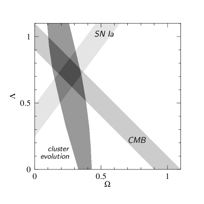
Figure 3.— Left: 68% and 90% confidence intervals on $\Omega_{m}$ and $\Lambda$ from evolution of the baryon mass function at $z>0.4$. Right: Comparison of the cluster evolution constraints with those from the distant supernovae and CMB. For each technique, we show only 68% confidence regions.

The resulting 68% and 90% confidence regions for parameters $\Omega_{m}$ and $\Lambda$ are shown in Fig. 3. The observed rate of the evolution of the baryon mass function defines a narrow band in the $(\Omega_{m},\Lambda)$ plane, slightly inclined to the $\Lambda$ axis:

$$\Omega_{m}+0.23\,\Lambda=0.41\pm 0.10.$$ (12)

The uncertainty in $\Omega_{m}$ for any fixed $\Lambda$ is $\pm 0.10$ at the 68% confidence level. For a flat cosmology, $\Omega_{m}+\Lambda=1$, we have $\Omega_{m}=0.24\pm 0.12$. Using only clusters with direct Chandra measurements of $M_{b}$, we obtain identical constraints on $\Omega_{m}$ and $\Lambda$, but the uncertainties are larger by a factor of $\sim 1.3$.

The band of acceptable values of $\Omega_{m}$ and $\Lambda$ approximately corresponds to a constant growth factor of linear density perturbations between $z\approx 0.55$ and $z\approx 0.05$, corresponding to the observed factor of 10 evolution of the mass function. For small values of $\Omega_{m}$, a significant growth factor is achieved only if $\Lambda$ is large (Carrol et al. 1992). For $\Lambda=0$ the required growth factor is achieved for $\Omega_{m}\approx 0.4$.

As has become a common practice, we compare our $(\Omega_{m},\Lambda)$ constraints with those provided by the observations of distant type Ia supernovae and the CMB fluctuations. The most robust constraint from the current CMB observations follows from the location of the first Doppler peak, which indicates that the Universe is nearly flat, $\Omega_{\text{tot}}=\Omega_{m}+\Lambda=1\pm 0.1$ (with a $0.4<h<0.9$ prior; Sievers et al. 2002, Rubiño-Martin et al. 2002). The distant supernovae data require a positive cosmological constant. We combine the SN Ia constraints from Riess et al. (1998) and Perlmutter et al. (1999): $\Lambda-1.33\,\Omega_{m}=0.37\pm 0.12$. The corresponding 68% confidence intervals are shown in the right panel of Fig. 3. Remarkably, the constraints from all three methods intersect in a small region, $\Omega_{m}=0.27\pm 0.085$, $\Lambda=0.73\pm 0.11$.

7. Discussion and conclusions

We have presented a new method of applying the models of the cluster evolution to observations at high redshifts. This method is based on easily observable baryon mass function. Unlike the studies based on the cluster temperature or luminosity functions, our method does not suffer from large uncertainties in the $M_{\text{tot}}-T$ and $M_{\text{tot}}-L$ relations. It uses only a physically motivated assumption that the baryon fraction in the cluster mass within the large radii is close to the universal value, $\Omega_{b}/\Omega_{m}$. Systematic uncertainties in this method are smaller and very different from those using the temperature or luminosity functions. Until improved observational techniques are able to normalize the scaling relations to a $10\%$ accuracy at all redshifts, modeling of the baryon mass function appears to be a promising method for deriving the cluster-based cosmological constraints.

The application of this method to the subsample of distant clusters from the 160 deg² survey results in a tight constraint on the combination of cosmological parameters $\Omega_{m}$ and $\Lambda$. This constraint intersects the current CMB and SN Ia constraints in a small area near $\Omega_{m}=0.3$ and $\Lambda=0.7$, showing a remarkable agreement of totally independent methods.

We note an excellent agreement of our cluster-derived cosmological parameter $\Omega_{m}$ with the results based on the X-ray measurements of the total mass and baryon fraction in the intermediate-redshift clusters (Allen et al. 2002). Also, there is a good agreement with those studies of the XTF evolution in the EMSS sample which use the normalization of the $M-T$ relation based on the X-ray mass measurements (e.g., Henry 2000). Such consistency indirectly confirms the validity of the X-ray cluster mass measurements.

Our method relies on the assumption that the baryon fraction in massive clusters does not evolve with redshift. This assumption is well-supported by numerical simulations. One issue of concern, however, is that these same simulations do not reproduce the observed evolution of the $M_{b}-T$ relation. At a fixed $T$, we observe $M_{b}\propto(1+z)^{-0.5\pm 0.4}$ for $\Omega_{m}=0.3$ and $\Lambda=0.7$ (Vikhlinin et al. 2002), which is significantly different from the expected evolution $(M_{b},M_{\text{tot}})\propto T^{3/2}(1+z)^{-3/2}$ (e.g., Bryan & Norman 1998). This may indicate that the baryon fraction in clusters evolves with redshift. However, it is much more likely that simulations simply do not reproduce the distribution of gas in the cluster central regions. These regions usually dominate in the observed emission-weighted $T$ but at the same time the gas there is especially prone to processes such as radiative cooling which can easily change $T$ but are unlikely to modify $M_{b}$ or $M_{\text{tot}}$.

The accuracy of our cosmological constraints is presently limited by the low number of the distant clusters. When new distant cluster samples from the Chandra, XMM, and extended ROSAT surveys become available, and more distant clusters are observed with adequate exposures by Chandra and XMM, even tighter cosmological constraints will be possible. Eventually, different methods (cluster evolution, CMB, SN Ia etc.) will start to disagree, which will lead to better understanding of the systematics and warrant more complicated theoretical models, e.g. those involving non-standard equations of state for the dark energy.

Appendix A Maximum likelihood fitting of the observed mass functions

The uncertainty intervals on the low- and high-redshift mass functions were obtained by the Maximum Likelihood analysis of the unbinned mass measurements. Our technique is presented in VVPb and briefly summarized below.

We assume that the observed mass function can be adequately described by the Schechter model,

$$f(M)=dN/dM=AM^{-\alpha}\exp(-M/M_{*}),$$ (A1)

in the narrow mass ranges of interest. The variation of parameters $A$, $\alpha$, and $M_{*}$ within the 3-parameter $N\%$ confidence intervals produces a band of the cumulative mass function models which we associate with the $N\%$ confidence band for the observed cumulative mass function.

The confidence intervals for parameters $A$, $\alpha$, and $M_{*}$ are obtained from the Maximum Likelihood modeling of the unbinned observed mass measurements. In the case of negligible mass measurement errors, the likelihood function is (cf. Cash 1979):

$$\log L=\sum_{i}\log\left(f(M_{i})V(M_{i})\right)-\int f(M)V(M)\,dM,$$ (A2)

where $M_{i}$ are the individual mass measurements, $V(M)$ is the sample volume as a function of mass (computed as described in § 3.1), and the integral is over the entire mass range. The quantity $C=-2\log L$ is statistically equivalent to $\chi^{2}$ (Cash 1979), therefore the uncertainties of the estimated parameters can be derived from the standard $\Delta\chi^{2}$ test. For example, a combined 68% confidence region for parameters $A$, $\alpha$, and $M_{*}$ is defined by the deviation $\Delta C=3.5$ from the minimum (the 68% probability point for the $\chi^{2}$ distribution with 3 degrees of freedom).

In the case of the finite mass measurement errors, the product $f(M)V(M)$ in (A2) should be convolved with the distribution of the measurement scatter. We assume that the scatter follows the log-normal distribution,

$$\frac{dP(\log M)}{d\log M}=\frac{\exp(-(\log M-\log\mu)^{2}/2\sigma^{2})}{(2\pi)^{1/2}\sigma},$$ (A3)

where $\mu$ is the true mass. The convolution of $f(M)V(M)$ with this distribution is

$$F(M,\sigma)=\int\frac{\exp(-(\log M-\log\mu)^{2}/2\sigma^{2})}{(2\pi)^{1/2}\sigma}f(\mu)V(\mu)\,d\log\mu$$ (A4)

and the likelihood function is

$$\log L=\sum_{i}\log\left(F(M_{i},\sigma_{i})\right)-\int_{M}F(M,\sigma(M))\,dM,$$ (A5)

where $\sigma_{i}$ is the log scatter of the $i$-th measurement and $\sigma(M)$ is the trend of the typical measurement scatter with mass.

The 68% confidence intervals for the cumulative mass function obtained with this technique are shown by grey bands in Fig. 2. For the low-redshift mass function, the mass measurement errors are small and we recover the pure Poisson scatter. The derived confidence interval for the distant mass function is wider than the Poisson scatter because the masses are less accurate.

The described technique automatically corrects any biases in the mass function determination which could arise from the measurement uncertainties (e.g., the Eddington bias). The close agreement between the model (not convolved with the measurement errors) and the data in Fig. 2 shows that such biases are small in our case. A bias could be expected because the mass function is steep, but is absent because of the rather flat distribution of the observed number of clusters in our sample per log interval of mass (this is the product of the intrinsic mass function and the selection function). The effect of the mass measurement uncertainties on the mass function is to smooth the distribution of $dN/d\log M$. If this distribution is flat, the net effect of the measurement uncertainties is zero. We verified the absence of biases in our case using Monte-Carlo simulations.

References

- (1)
- (2) Allen, S. W., Schmidt, R. W., & Fabian, A. C. 2002, MNRAS, 334, L11
- (3)
- (4) Bialek, J. J., Evrard, A. E., & Mohr, J. J. 2001, ApJ, 555, 597
- (5)
- (6) Blanchard, A., Sadat, R., Bartlett, J. G., & Le Dour, M. 2000, A&A, 362, 809
- (7)
- (8) Bond, J. R. & Efstathiou, G. 1984, ApJ, 285, L45
- (9)
- (10) Borgani, S. et al. 2001, ApJ, 561, 13
- (11)
- (12) Bryan, G. L. & Norman, M. L. 1998, ApJ, 495, 80
- (13)
- (14) Burles, S., Nollett, K. M., & Turner, M. S. 2001, ApJ, 552, L1
- (15)
- (16) Carroll, S. M., Press, W. H., & Turner, E. L. 1992, ARA&A, 30, 499
- (17)
- (18) Cash, W. 1979, ApJ, 228, 939
- (19)
- (20) Cavaliere, A., Menci, N., & Tozzi, P. 1997, ApJ, 484, L21
- (21)
- (22) Donahue, M. & Voit, G. M. 1999, ApJ, 523, L137
- (23)
- (24) Ebeling, H. et al. 2000, ApJ, 534, 133
- (25)
- (26) Eisenstein, D. J. & Hu, W. 1998, ApJ, 496, 605
- (27)
- (28) Eke, V. R., Cole, S., Frenk, C. S., & Henry, J. P. 1998, MNRAS, 298, 1145
- (29)
- (30) Evrard, A. E. 1989, ApJ, 341, L71
- (31)
- (32) Evrard, A. E. et al. 2002, ApJ, 573, 7
- (33)
- (34) Finoguenov, A., Reiprich, T. H., & Böhringer, H. 2001, A&A, 368, 749
- (35)
- (36) Fischer, P. & Tyson, J. A. 1997, AJ, 114, 14
- (37)
- (38) Fukugita, M., Hogan, C. J. & Peebles, P. J. E. 1998, ApJ, 503, 518
- (39)
- (40) Gioia, I. M., Maccacaro, T., Schild, R. E., Wolter, A., Stocke, J. T., Morris, S. L., & Henry, J. P. 1990, ApJS, 72, 567
- (41)
- (42) Gioia, I. M., Henry, J. P., Mullis, C. R., Voges, W., Briel, U. G., Böhringer, H., & Huchra, J. P. 2001, ApJ, 553, L105
- (43)
- (44) Hamilton, A. J. S. 2001, MNRAS, 322, 419
- (45)
- (46) Henry, J. P. & Arnaud, K. A. 1991, ApJ, 372, 410
- (47)
- (48) Henry, J. P., Gioia, I. M., Maccacaro, T., Morris, S. L., Stocke, J. T., & Wolter, A. 1992, ApJ, 386, 408
- (49)
- (50) Henry, J. P. 1997, ApJ, 489, L1
- (51)
- (52) Henry, J. P. 2000, ApJ, 534, 565
- (53)
- (54) Horner, D. J., Mushotzky, R. F., & Scharf, C. A. 1999, ApJ, 520, 78
- (55)
- (56) Jenkins, A., Frenk, C. S., White, S. D. M., Colberg, J. M., Cole, S., Evrard, A. E., Couchman, H. M. P., & Yoshida, N. 2001, MNRAS, 321, 372
- (57)
- (58) Lewis, A. D., Stocke, J. T., Ellingson, E., & Gaidos, E. J. 2002, ApJ, 566, 744
- (59)
- (60) Markevitch, M. & Vikhlinin, A. 1997, ApJ, 491, 467
- (61)
- (62) Mathiesen, B., Evrard, A. E., & Mohr, J. J. 1999, ApJ, 520, L21
- (63)
- (64) Nevalainen, J., Markevitch, M., & Forman, W. 2000, ApJ, 532, 694
- (65)
- (66) Nichol, R. C., Holden, B. P., Romer, A. K., Ulmer, M. P., Burke, D. J., & Collins, C. A. 1997, ApJ, 481, 644
- (67)
- (68) Peebles, P. J. E. 1980, The Large-Scale Structure of the Universe (Princeton Univ. Press)
- (69)
- (70) Pen, U. 1997, New Astronomy, 2, 309
- (71)
- (72) Perlman, E. S., Horner, D. J., Jones, L. R., Scharf, C. A., Ebeling, H., Wegner, G., & Malkan, M. 2002, ApJS, 140, 265
- (73)
- (74) Perlmutter, S. et al. 1999, ApJ, 517, 565
- (75)
- (76) Press, W. H. & Schechter, P. 1974, ApJ, 187, 425
- (77)
- (78) Reichart, D. E., Nichol, R. C., Castander, F. J., Burke, D. J., Romer, A. K., Holden, B. P., Collins, C. A., & Ulmer, M. P. 1999, ApJ, 518, 521
- (79)
- (80) Reiprich, T. H. & Böhringer, H. 2002, ApJ, 567, 716
- (81)
- (82) Riess, A. G. et al. 1998, AJ, 116, 1009
- (83)
- (84) Rosati, P., Della Ceca, R., Norman, C., & Giacconi, R. 1998, ApJ, 492, L21
- (85)
- (86) Rosati, P., Borgani, S. & Norman, C. 2002, ARA&A, 40, 539
- (87)
- (88) Rubiño-Martin, J. A. et al. 2002, MNRAS (submitted, astro-ph/0205367)
- (89)
- (90) Sasaki, S. 1996, PASJ, 48, L119
- (91)
- (92) Seljak, U. & Zaldarriaga, M. 1996, ApJ, 469, 437
- (93)
- (94) Sievers, J. L. 2002, ApJ (submitted; astro-ph/0205387)
- (95)
- (96) Sunyaev, R. A. 1971, A&A, 12, 190
- (97)
- (98) Vikhlinin, A., McNamara, B. R., Forman, W., Jones, C., Quintana, H., & Hornstrup, A. 1998, ApJ, 502, 558
- (99)
- (100) Vikhlinin, A., Forman, W., & Jones, C. 1999, ApJ, 525, 47
- (101)
- (102) Vikhlinin, A. et al. 2000, in Proceedings of Large Scale Structure in the X-ray Universe, eds. Plionis, M. & Georgantopoulos, I., (Atlantisciences, Paris)
- (103)
- (104) Vikhlinin, A., VanSpeybroeck, L., Markevitch, M., Forman, W. R., & Grego, L. 2002, ApJ, 578, L107
- (105)
- (106) Voevodkin, A. A., Vikhlinin, A. A., & Pavlinsky, M. N. 2002a, Astronomy Letters, 28, 366 (VVPa)
- (107)
- (108) Voevodkin, A. A., Vikhlinin, A. A., & Pavlinsky, M. N. 2002b, Astronomy Letters, 28, 793 (VVPb)
- (109)
- (110) White, S. D. M., Navarro, J. F., Evrard, A. E., & Frenk, C. S. 1993, Nature, 366, 429
- (111)