The linear MHD Taylor-Couette instability for liquid sodium

Abstract

The linear stability of MHD Taylor-Couette flow of infinite vertical extension is considered for liquid sodium with its small magnetic Prandtl number Pm of order of $10^{-5}$. The calculations are performed for a container with $\hat{\eta}=0.5$ with an axial uniform magnetic field excluding counter rotating cylinders. The sign of the constant $a$ in the basic rotation law $\Omega=a+b/R^{2}$ strongly influences the presented results. It is negative for resting outer cylinder. The main point here is that the subcritical excitation which occurs for large Pm disappears for small Pm (cf. Fig. 3). This is the reason that the existence of the magnetorotational instability remained unknown over decades.

For rotating outer cylinder the limiting case $a=0$ (i.e. $\hat{\mu}=\hat{\eta}^{2}$) plays an exceptional role. The hydrodynamic instability starts to disappear while the hydromagnetic instability exists with minimal Reynolds numbers at certain Hartmann numbers of the magnetic field. These Reynolds numbers exactly scale with Pm^-1/2 resulting in moderate values of order $10^{4}$ for Pm=10^-5. However, already for the smallest positive value of $a$ the Reynolds numbers start to scale as 1/Pm leading to much higher values of order $10^{6}$ for Pm=10^-5. Hence, for outer cylinders rotating faster than the limit $a=0$ it is exclusively the magnetic Reynolds number Rm which directs the excitation of the instability. They are resulting as lower for insulating walls (‘vacuum’) than for conducting walls. Generally, the magnetic Reynolds numbers for liquid sodium have to exceed values of order 10 leading to frequencies of about 20 Hz for the rotation of the inner cylinder if containers with (say) 10 cm radius are considered. The required magnetic fields are about 1000 Gauss.

Also nonaxisymmetric modes have been considered. With vacuum boundary conditions their excitation is always more difficult than the excitation of axisymmetric modes; we never observed a crossover of the lines of marginal stability. For conducting walls, however, such crossovers exist for both resting and rotating outer cylinders, and this might be essential for future dynamo experiments. In this case, however, the instability also can onset in form of oscillating axisymmetric patterns of flow and field and the Reynolds numbers of these solutions are lower than the Reynolds numbers for the stationary solutions.

I Introduction

The longstanding problem of the generation of turbulence in various hydrodynamically stable situations has found a solution in recent years with the MHD shear flow instability, also called magnetorotational instability (MRI), in which the presence of a magnetic field has a destabilizing effect on a differentially rotating flow with the angular velocity decreasing outwards. The MRI has been formulated decades ago V59 ; C61 for ideal Taylor-Couette flow, but its importance as the source of turbulence in accretion discs with differential (Keplerian) rotation was first recognized by Balbus and Hawley, BH91 .

However, the MRI has never been observed in the laboratory DO60 ; DO62 ; DC64 ; B70 . After Goodman and Ji GJ01 was the absence of MRI due to the small magnetic Prandtl number approximation used in C61 . The magnetic Prandtl number Pm is really very small under laboratory conditions ($\sim 10^{-5}$ and smaller, see Table 1).

Table 1: Parameters of the fluids suitable for MHD experiments taken from C61 and NPCNB02

	$\rho$ [g/cm3]	$\nu$ [cm2/s]	$\eta$ [cm2/s]	Pm
Mercury	5.4	1.1$\cdot 10^{-3}$	7600	1.4$\cdot 10^{-7}$
Gallium	6.0	3.2$\cdot 10^{-3}$	2060	1.5$\cdot 10^{-6}$
Sodium	0.92	7.1$\cdot 10^{-3}$	810	0.88$\cdot 10^{-5}$

A proper understanding of this phenomenon is very important for possible future experiments, including Taylor-Couette flow dynamo experiments.

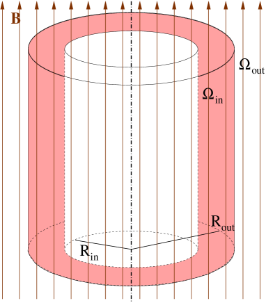
Figure 1: Cylinder geometry of the Taylor-Couette flow with axial magnetic field.

The simple model of uniform density fluid contained between two vertically-infinite rotating cylinders is used with constant magnetic field parallel to the rotation axis. For viscous flows the most general form of the rotation law $\Omega(R)$ in the fluid is

$${\Omega}(R)=a+b/{R}^{2},$$ (1)

where $a$ and $b$ are two constants related to the angular velocities $\Omega_{\rm in}$ and $\Omega_{\rm out}$ with which the inner and the outer cylinders are rotating and $R$ is the distance from the rotation axis. If $R_{\rm in}$ and $R_{\rm out}$ ($R_{\rm out}>R_{\rm in}$) are the radii of the two cylinders then

$$a={\hat{\mu}-{\hat{\eta}}^{2}\over 1-{\hat{\eta}}^{2}}{\Omega}_{\rm in}\ \ \ \ \ {\rm and}\ \ \ \ b=R_{\rm in}^{2}{1-\hat{\mu}\over 1-{\hat{\eta}}^{2}}{\Omega}_{\rm in}$$ (2)

with

$$\hat{\mu}={\Omega}_{\rm out}/\Omega_{\rm in}\qquad{\rm and}\qquad\hat{\eta}=R_{\rm in}/R_{\rm out}.$$ (3)

Following the Rayleigh stability criterion, $d(R^{2}{\Omega})^{2}/dR>0$, rotation laws are hydrodynamically stable for $a>0$, i.e. $\hat{\mu}>\hat{\eta}^{2}$. They should in particular be stable for resting inner cylinder, i.e. $\hat{\mu}\to\infty$. Richard and Zahn RZ99 focused attention to the experimental results of Wendt W1933 who found nonlinear instability for this case for Reynolds numbers of order 10⁵. The finite-amplitude instability of hydrodynamically stable rotation laws must therefore remain in the astrophysical discussion. However, later experiments with very similar Taylor-Couette flow experiments for resting inner cylinder demonstrated the results of Wendt as due to rather imperfect container constructions and the flow remained laminar even for Reynolds numbers up to 10⁶, Sch59 .

One of the targets in the present paper is the axisymmetry of the excited modes. We have shown in SRS02 that for containers with conducting boundaries it happens for sufficiently strong magnetic fields that the mode with the lowest eigenvalue (i.e. the lowest Reynolds number) is a nonaxisymmetric mode. As an impressive example, in Fig. 2 for Pm=0.01 the crossover of the instability lines for axisymmetric and nonaxisymmetric modes is shown for Hartmann numbers of about 400 (see ).

Figure 2: Instability lines for axisymmetric (solid) and nonaxisymmetric modes (m=1, dashed line) for conducting walls and Pm=0.01 ($\hat{\eta}=0.5$).

Despite of its general meaning this behavior is only known so far for conducting walls and for magnetic Prandtl numbers not smaller than 10^-2 (see KGDIP66 ). For possible laboratory experiments we have to extend, however, the computations to insulating boundaries (vacuum) and to much smaller magnetic Prandtl numbers Pm.

The equations, therefore, are solved here mainly for the single small magnetic Prandtl number Pm $=10^{-5}$ very close to the value for liquid sodium (see Table 1). The aspect ratio of the container walls radii in the present paper is fixed to $\hat{\eta}=0.5$.

II Basic equations

The MHD equations which have to be solved are

$${\partial\mbox{\boldmath$u$}\over\partial t}+(\mbox{\boldmath$u$}\nabla)\mbox{\boldmath$u$}=-{1\over\rho}\nabla p+\nu\Delta\mbox{\boldmath$u$}+\mbox{\boldmath$J$}\times\mbox{\boldmath$B$}$$ (4)

and

$${\partial\mbox{\boldmath$B$}\over\partial t}={\rm curl}(\mbox{\boldmath$u$}\times\mbox{\boldmath$B$})+\eta\Delta\mbox{\boldmath$B$},$$ (5)

with the electric current $J={\rm curl}\mbox{\boldmath$B$}/\mu_{0}$ and ${\rm div}\mbox{\boldmath$u$}={\rm div}\mbox{\boldmath$B$}=0$. They are considered in cylindrical geometry with $R$, $\phi$, and $z$ as the cylindrical coordinates. A viscous electrically-conducting incompressible fluid between two rotating infinite cylinders in the presence of a uniform magnetic field parallel to the rotation axis leads to the basic solution $U_{R}=U_{z}=B_{R}=B_{\phi}=0,B_{z}=B_{0}={\rm const.,}\ {\rm and}\ U_{\phi}=aR+b/R$, with $U$ as the flow and $B$ as the magnetic field. We are interested in the stability of this solution. The perturbed state of the flow may be described by $u_{R}^{\prime},\;u_{\phi}^{\prime},\;u_{z}^{\prime},\;B_{R}^{\prime},\;B_{\phi}^{\prime},\;B_{z}^{\prime},\;p^{\prime}$ with $p^{\prime}$ as the pressure perturbation.

Here only the linear stability problem is considered. By analyzing the disturbances into normal modes the solutions of the linearized hydromagnetic equations are of the form

$$\mbox{\boldmath$B$}^{\prime} = \mbox{\boldmath$B$}(R)\ {\rm e}^{{\rm i}(m\phi+kz-\omega t)},$$

$$\mbox{\boldmath$u$}^{\prime} = \mbox{\boldmath$u$}(R)\ {\rm e}^{{\rm i}(m\phi+kz-\omega t)}.$$ (6)

From hereon all dashes have been omitted from the notations of fluctuating quantities. Only marginal stability will be considered hence the imaginary part of $\omega$, i.e. ${\cal I}(\omega)$, always vanishes. We use

$$H=\sqrt{R_{\rm in}(R_{\rm out}-R_{\rm in})}$$ (7)

as the unit of length, the $\eta/H$ as the unit of perturbed velocity and $B_{0}$ as the unit of perturbed magnetic field and work with the magnetic Prandtl number

$${\rm Pm}={\nu\over\eta},$$ (8)

with $\nu$ the kinematic viscosity and $\eta$ the magnetic diffusivity. Note $H^{-1}$ also as the unit of wave numbers and $\nu/H^{2}$ as the unit of frequencies. After elimination of both pressure fluctuations and the fluctuations of the vertical magnetic field, $B^{\prime}_{z}$, the linearized equations are

$${\partial u_{R}\over\partial R}+{u_{R}\over R}+{{\rm i}m\over R}u_{\phi}+{\rm i}ku_{z}=0,$$ (9)

$${\partial^{2}u_{\phi}\over\partial R^{2}}+{1\over R}{\partial u_{\phi}\over\partial R}-{u_{\phi}\over R^{2}}-\left({m^{2}\over R^{2}}+k^{2}\right)u_{\phi}-$$

$$-{\rm i}\left(m{\rm Re}{\Omega\over\Omega_{\rm in}}-\omega\right)u_{\phi}+{2{\rm i}m\over R^{2}}u_{R}-{\rm Re}{1\over R}{\partial\over\partial R}\left(R^{2}{\Omega\over\Omega_{\rm in}}\right)u_{R}$$ (10)

$$-{m\over k}\left[{1\over R}{\partial^{2}u_{z}\over\partial R^{2}}+{1\over R^{2}}{\partial u_{z}\over\partial R}-\left({m^{2}\over R^{2}}+k^{2}\right){u_{z}\over R}-\right.$$

$$\left.-{\rm i}\left(m{\rm Re}{\Omega\over\Omega_{\rm in}}-\omega\right){u_{z}\over R}\right]+{m\over k}{\rm Ha}^{2}\left[{1\over R}{\partial B_{R}\over\partial R}+{B_{R}\over R^{2}}\right]+$$

$$+{{\rm i}\over k}{\rm Ha}^{2}\left({m^{2}\over R^{2}}+k^{2}\right)B_{\phi}=0,$$

$${\partial^{3}u_{z}\over\partial R^{3}}+{1\over R}{\partial^{2}u_{z}\over\partial R^{2}}-{1\over R^{2}}{\partial u_{z}\over\partial R}-\left({m^{2}\over R^{2}}+k^{2}\right){\partial u_{z}\over\partial R}+$$

$$+{2m^{2}\over R^{3}}u_{z}-{\rm i}\left(m{\rm Re}{\Omega\over\Omega_{\rm in}}-\omega\right){\partial u_{z}\over\partial R}-{\rm i}m{\rm Re}{\partial\over\partial R}\left({\Omega\over\Omega_{\rm in}}\right)u_{z}$$ (11)

$$-{\rm Ha}^{2}\left[{\partial^{2}B_{R}\over\partial R^{2}}+{1\over R}{\partial B_{R}\over\partial R}-{B_{R}\over R^{2}}-k^{2}B_{R}+\right.$$

$$\left.+{{\rm i}m\over R}{\partial B_{\phi}\over\partial R}-{{\rm i}m\over R^{2}}B_{\phi}\right]-{\rm i}k\left[{\partial^{2}u_{R}\over\partial R^{2}}+{1\over R}{\partial u_{R}\over\partial R}-{u_{R}\over R^{2}}-\right.$$

$$\left.-\left(k^{2}+{m^{2}\over R^{2}}\right)u_{R}\right]-k\left(m{\rm Re}{\Omega\over\Omega_{\rm in}}-\omega\right)u_{R}-$$

$$-2{km\over R^{2}}u_{\phi}-2{\rm i}k{\rm Re}{\Omega\over\Omega_{\rm in}}u_{\phi}=0,$$

$${\partial^{2}B_{R}\over\partial R^{2}}+{1\over R}{\partial B_{R}\over\partial R}-{B_{R}\over R^{2}}-\left({m^{2}\over R^{2}}+k^{2}\right)B_{R}-$$ (12)

$$-{2{\rm i}m\over R^{2}}B_{\phi}-{\rm i}{\rm Pm}\left(m{\rm Re}{\Omega\over\Omega_{\rm in}}-\omega\right)B_{R}+{\rm i}ku_{R}=0,$$

$${\partial^{2}B_{\phi}\over\partial R^{2}}+{1\over R}{\partial B_{\phi}\over\partial R}-{B_{\phi}\over R^{2}}-\left({m^{2}\over R^{2}}+k^{2}\right)B_{\phi}+$$ (13)

$$+{2{\rm i}m\over R^{2}}B_{R}-{\rm i}{\rm Pm}\left(m{\rm Re}{\Omega\over\Omega_{\rm in}}-\omega\right)B_{\phi}+{\rm i}ku_{\phi}+$$

$$+{\rm Pm}\ {\rm Re}\ R{\partial\Omega/\Omega_{\rm in}\over\partial R}B_{R}=0.$$

Here the Reynolds number Re and the Hartmann number Ha are defined as

$${\rm Re}={{\Omega}_{\rm in}R_{\rm in}(R_{\rm out}-R_{\rm in})\over\nu}$$ (14)

and

$${\rm Ha}=B_{0}\sqrt{R_{\rm in}(R_{\rm out}-R_{\rm in})\over\mu_{0}\rho\nu\eta}.$$ (15)

For given Hartmann number and magnetic Prandtl number in the present paper we shall compute with a linear theory the critical Reynolds number of the rotation of the inner cylinder, also for various mode numbers $m$.

III Boundary conditions, numerics

An appropriate set of ten boundary conditions is needed to solve the system (9)$\dots$(13). Always no-slip conditions for the velocity on the walls are used, i.e. $u_{R}=u_{\phi}=du_{R}/dR=0.$ The boundary conditions for the magnetic field depend on the electrical properties of the walls. The tangential currents and the radial component of the magnetic field vanish on conducting walls hence $dB_{\phi}/dR+B_{\phi}/R=B_{R}=0.$ These boundary conditions may also hold both for $R=R_{\rm in}$ and for $R=R_{\rm out}$.

The homogeneous set of equations (9)$\dots$(13) together with the boundary conditions determine the eigenvalue problem of the form ${\cal L}(k,m,{\rm Re},{\rm Ha},{\cal{R}}(\omega))=0$ for given Pm. The real part of $\omega$, i.e. ${\cal{R}}(\omega)$, describes a drift of the pattern along the azimuth which only exists for nonaxisymmetric flows. For axisymmetric flows $(m=0)$ the real part of $\omega$, i.e. ${\cal R}(\omega)$, is zero for stationary patterns of flow and field and it is nonzero for oscillating solutions, which are called overstability. $\cal L$ is a complex quantity, both its real part and its imaginary part must vanish for the critical Reynolds number. The latter is minimized by choice of the wave number $k$. ${\cal R}(\omega)$ is the second quantity which is fixed by the eigen equation.

The system is approximated by finite differences with typically 200 radial grid points. The resulting determinant, $\cal L$, takes the value zero if and only if the values Re are the eigenvalues. We can also stress that the results are numerically robust as an increase of the number of grid points does not change the results remarkably. For a fixed Hartmann number, a fixed Prandtl number and a given vertical wave number $k$ we find the eigenvalues of the equation system. They are always minimal for a certain wave number which by itself defines the marginally unstable mode. The corresponding eigenvalue is the desired Reynolds number.

The situation changes for insulating walls. The magnetic field must match the external magnetic field for vacuum. It is known for this case that the boundary conditions for axisymmetric solutions strongly differ from those for nonaxisymmetric solutions (see EMR90 ). The condition ${\rm curl}_{R}{\mbox{\boldmath$B$}}=0$ in vacuum immediately provides

$$B_{\phi}={m\over kR}B_{z}$$ (16)

at $R=R_{\rm in}$ and $R=R_{\rm out}$. From the solution of the potential equation $\Delta\psi=0$ one finds

$$B_{R}+{{\rm i}B_{z}\over I_{m}(kR)}\left({m\over kR}I_{m}(kR)+I_{m+1}(kR)\right)=0$$ (17)

for $R=R_{\rm in}$ and

$$B_{R}+{{\rm i}B_{z}\over K_{m}(kR)}\left({m\over kR}K_{m}(kR)-K_{m+1}(kR)\right)=0$$ (18)

for $R=R_{\rm out}$. $I_{m}$ and $K_{m}$ are the modified Bessel functions (with different behavior at $R\to 0$ and $R\to\infty$). One can eliminate with div$B$=0 the vertical component $B_{z}$ of the magnetic field in the boundary conditions (16)…(18).

IV Results

The following results concern different aspects of the MHD Taylor-Couette problem for small magnetic Prandtl number Pm. In Section A the main realization of the case $a<0$ (here with resting outer cylinder, i.e. $\hat{\mu}=0$) is considered. There is instability even without magnetic fields so that the bifurcation lines start at the y-axis. In Section B the special case $a=0$ is considered with very surprising results. The Section C presents the results for the two experiments with $\hat{\mu}=0$ and $\hat{\mu}=0.33$ with respect to the axisymmetry of the eigenmodes. In Section D the existence of oscillating modes is discussed, i.e. the case of overstability for small magnetic Prandtl numbers.

IV.1 Subcritical excitation for large Pm ($\mbox{\boldmath$a$}{\bf<0}$)

Figure 3: Marginal stability lines for axisymmetric modes with resting outer cylinder of conducting material. The shaded area denotes subcritical excitations of unstable axisymmetric modes by the external magnetic field.

Figure 3 shows the stability lines for axisymmetric modes for containers with conducting walls and with resting outer cylinder for fluids of various magnetic Prandtl number. Only the vicinity of the classical hydrodynamic solution with Re $=68$ is shown. There is a strong difference of the geometry of the bifurcation lines for Pm $\lower 1.72218pt\hbox{$\;\buildrel>\over{\scriptstyle\sim}\;$}1$ and Pm $<1$. In the latter case, for fluids with low electrical conductivity the magnetic field only suppresses the instability so that all the critical Reynolds numbers exceed the value 68, and this the more the stronger the magnetic field is.

For sufficiently small magnetic Prandtl number the stability lines hardly differ, which is the situation already considered by Chandrasekhar C61 without any indication of magnetorotational instability.

The opposite is true for Pm $\lower 1.72218pt\hbox{$\;\buildrel>\over{\scriptstyle\sim}\;$}1$. Note that in Fig. 3 for materials with high electrical conductivity the resulting critical Reynolds numbers are smaller than Re $=68$. The magnetic field with small Hartmann numbers support instability patterns rather than to suppress them. This effect becomes more effective for increasing Pm but it vanishes for stronger magnetic fields. Obviously, the MRI only exists for weak magnetic fields and high enough electrical conductivity and/or molecular viscosity (when the fields can be considered as frozen in and/or enough viscosity prevents the action of the Taylor-Proudman theorem).

Note that the subcritical excitation of Taylor vortices only works for weak magnetic fields. The upper limits of the possible Hartmann numbers can be observed for the magnetic Prandtl numbers 1 and 10 in Fig. 4.

Figure 4: Critical Reynolds number versus $\hat{\eta}$ for $\hat{\mu}=\hat{\eta}^{2}$ and Pm$=1$.

After our computations the subcritical excitation of Taylor vortices for weak magnetic fields requires rather high magnetic Prandtl numbers. The microscopic values for Pm are orders of magnitudes smaller than unity, so that there should be no chance to realize the subcritical excitation of Taylor vortices by experiments. However, the speculation may be allowed whether really the microscopic Pm is the basic input. The scenario is also interesting whether possible finite-amplitude hydrodynamic instabilities provide some kind of background turbulence which can be considered as modifying the value of the magnetic Prandtl number, NPCNB02 . The turbulence influences both the viscosity values and the magnetic-diffusivity values so that

$${\rm Pm}\to{\rm Pm}_{\rm eff}={\nu+\nu_{\rm T}\over\eta+\eta_{\rm T}}\simeq{\nu_{\rm T}\over\eta_{\rm T}}$$ (19)

with $\nu_{\rm T}$ and $\eta_{\rm T}$ as the eddy viscosity and the eddy diffusivity, resp. Because of the existence of the pressure term in the momentum equation, both quantities are not identical. We do not have precise knowledge about the effective turbulent magnetic Prandtl number but it has been demonstrated that values of order 0.1 or somewhat larger should not be unlikely, R89 . Insofar if such speculations are not too far from the reality, it is not completely clear that the subcritical excitation of Taylor vortices which we have presented in Fig. 4 is unobservable in general.

IV.2 The case ${\bf a=0}$ ($\mbox{\boldmath$\hat{\mu}$}=\mbox{\boldmath$\hat{\eta}^{2}$}$)

There is a universal scaling on Pm for the special case with $a=0$ in the basic flow profile (1), i.e. for $\hat{\mu}=\hat{\eta}^{2}$. Then the term with $\partial(R^{2}\Omega)/\partial R$ in Eq. (10) vanishes and for $m=\omega=0$ one finds that the quantities $u_{R},u_{z},B_{R}$ and $B_{z}$ are scaling as Pm^-1/2 while $u_{\phi},B_{\phi},k$ Ha scale as Pm⁰. Then also the Reynolds number for the axisymmetric modes scales as

$${\rm Re}\propto{\rm Pm}^{-1/2}.$$ (20)

The scaling does not depend on the boundary conditions as these for $m=0$ also comply with the relations.

The result (20) has numerically been found by Willis and Barenghi for vacuum boundary conditions, WB02 . However, Rüdiger and Shalybkov RS02 for $a>0$ ($\hat{\mu}>\hat{\eta}^{2}$) found the much steeper scaling

$${\rm Re}\propto{\rm Pm}^{-1},$$ (21)

resulting in the surprisingly simple relation

$${\rm Rm}\propto{\rm const.}$$ (22)

for the magnetic Reynolds number ${\rm Rm}={{\Omega}_{\rm in}R_{\rm in}(R_{\rm out}-R_{\rm in})/\eta}$ and

$${\rm Ha}\propto{\rm Pm}^{-1/2}$$ (23)

resulting in

$${\rm Ha}^{*}\propto{\rm const.}$$ (24)

for ${\rm Ha}^{*}=B_{0}\sqrt{R_{\rm in}(R_{\rm out}-R_{\rm in})/\mu_{0}\rho\eta^{2}}$ (Lundquist number, see RS02 ). In case of small magnetic Prandtl number the exact value of the microscopic viscosity is totally unimportant for the excitation of the instability. In consequence, however, the corresponding Reynolds numbers for the MRI seem to differ by 2 orders of magnitude, i.e. 10⁴ and 10⁶. Insofar, experiments with $\hat{\mu}=\hat{\eta}^{2}$ seem to look much more promising than experiments with $\hat{\mu}>\hat{\eta}^{2}$.

Unfortunately, this challenging possibility cannot be utilized in experiments. The critical Reynolds number for $\hat{\mu}=\hat{\eta}^{2}$ and Pm=1 as a function of $\hat{\eta}$ is given in Fig. 4. The total minimum of the Reynolds number is 54.4 for $\hat{\eta}=0.27$ so that after (20) one expects the value 1.7$\cdot 10^{4}$ for the Reynolds number for Pm$=10^{-5}$. Fig. 5 shows the behavior of this result in the vicinity of $\hat{\mu}=\hat{\eta}^{2}$. There is a vertical jump from 10⁴ to 10⁶ in an extremely small interval of the abscissa. This sharp transition does not exist for Pm=1, it is only due to the very small value of Pm. For this case in Fig. 5 the coexistence of both hydrodynamic and hydromagnetic instability is also presented.

Figure 5: Critical Reynolds numbers for the Taylor-Couette flow versus $\hat{\mu}$ for $\hat{\eta}=0.27$ and Pm=1 (left) and Pm=$10^{-5}$ (right). The curve for the hydrodynamic instability (Ha=0) is dashed and the hydromagnetic curve (Ha$>$0) is solid. The dotted line denotes the location of $a$=0, i.e. $\hat{\mu}=\hat{\eta}^{2}$.

The jump profile for Pm$=10^{-5}$ in Fig. 5 (right) makes it clear that such experiments with $\hat{\mu}=\hat{\eta}^{2}$ are not possible. Even the smallest deviation from the condition $\hat{\mu}=\hat{\eta}^{2}$ drastically changes the excitation condition. For $\hat{\mu}$ smaller than $\hat{\eta}^{2}$ (negative deviations) the hydrodynamic instability sets in and for $\hat{\mu}$ slightly exceeding $\hat{\eta}^{2}$ (positive deviations) the Reynolds number suddenly jumps by two orders of magnitudes.

IV.3 Excitation of nonaxisymmetric modes

Figure 6: Insulating walls (vacuum): Stability lines for axisymmetric ($m=0$, solid lines) and nonaxisymmetric instability modes with $m=1$ (dashed). LEFT: resting outer cylinder, RIGHT: rotating outer cylinder (33%).

Figure 7: Conducting walls: Stability lines for axisymmetric ($m=0$, solid lines) and nonaxisymmetric instability modes with $m=1$ (dashed). LEFT: resting outer cylinder, RIGHT: rotating outer cylinder (33 %).

Table 2: Coordinates of the absolute minima in Figs. 6 and 7 for rotating outer cylinder ($\hat{\mu}=0.33$)

	conducting walls	insulating walls
Reynolds number	$2.13\cdot 10^{6}$	$1.42\cdot 10^{6}$
magnetic Reynolds number	21	14
Hartmann number	$1100$	$1400$
Lundquist number	3.47	4.42

Let us now concentrate to the small magnetic Prandtl number for liquid sodium, i.e. Pm $=10^{-5}$. We start with the results for containers with insulating walls and outer cylinders at rest, (Fig. 6a). There are then linear instabilities even without magnetic fields. For Ha$=0$ solutions for $m=0$ (Re$=68$) and $m=1$ (Re$=75$) are known, see SRS02 . The axisymmetric mode possesses the lowest eigenvalue. This is also true for nonvanishing magnetic field; we do not find any crossover of the instability lines for axisymmetric and nonaxisymmetric modes. The same is true for containers with rotating outer cylinder (Fig. 6b). For growing $\hat{\mu}$ the Reynolds number for the hydrodynamic solution moves upwards, reaching infinity for $\hat{\mu}=\hat{\eta}^{2}=0.25$ (here). The MRI is represented by characteristic minima, in our case for $\hat{\mu}=0.33$ at Hartmann numbers of order $10^{3}$ and Reynolds numbers of order $10^{6}$. The exact coordinates of the minima are given in Table 2.

In order to characterize the Hartmann numbers note that for liquid sodium

$$B=2.2{{\rm Ha}\over R_{\rm out}/10{\rm cm}}\ {\rm Gauss}.$$ (25)

Hence, for $R_{\rm out}\simeq 22$ the magnetic field and the Hartmann number have the same numerical values. With $\nu=10^{-2}$ cm²/s and $\hat{\eta}$=0.5 it follows from (14) and (15)

$$f_{\rm in}=64{{\rm Re}/10^{6}\over\left(R_{\rm out}/10{\rm cm}\right)^{2}}\ {\rm Hz}$$ (26)

for the frequency of the inner cylinder. Hence, a container with an outer radius of 22 cm (see above) and an inner radius of 11 cm filled with liquid sodium and embedded in vacuum requires a rotation of about 19 Hz in order to find the MRI. Following (25) the required magnetic field is about 1400 Gauss.

Figure 8: The same as in Fig. 7a but with the inclusion of oscillating axisymmetric modes (overstability) appearing here for lower Reynolds numbers.

The results for containers with conducting walls are given in Fig. 7. Note that the minimal Reynolds numbers given in Fig. 7b are higher than for insulating cylinder walls. The influence of the boundary conditions is not as small as expected. The main difference between the two sorts of boundary conditions, however, is the existence of crossovers of the instability lines for $m=0$ and $m=1$ in case of conducting walls. For both resting and rotating outer cylinder Hartmann numbers exist above which the nonaxisymmetric mode possesses a lower Reynolds number than the axisymmetric mode. We have already shown the existence of such crossovers for conducting walls for $1\leq{\rm Pm}\leq 0.01$ in SRS02 . It is now clear that the occurrence of nonaxisymmetric solutions as the preferred modes is a rather general phenomenon for containers with conducting walls which can become important for the design of future dynamo experiments (Cowling theorem).

IV.4 Excitation of oscillating modes

There are not only stationary patterns of flow and field possible but the instability can also onset in form of oscillating solutions. This effect is called overstability. In case of rotating convection between two layers heated from below the onset of the instability in form of oscillating solutions even possesses the lowest eigenvalues for certain Prandtl numbers, C61 . We find a very similar behavior for the MHD Taylor-Couette flow between conducting cylinders for resting outer cylinder (see Fig. 8). It is a pair of waves traveling in positive and negative $z$-direction. Note that the cylinder considered here has no bound in vertical direction. If the cylinder is finite, however, the possibility exists that traveling waves might be combined to standing waves.

References

- (1) E. P. Velikhov, Sov. Phys. JETP 9, 995 (1959).
- (2) S. Chandrasekhar, Hydrodynamic and Hydromagnetic Stability (Clarendon, Oxford, 1961).
- (3) S. A. Balbus and J. F. Hawley, Astrophys. J. 376, 214 (1991).
- (4) R. J. Donnelly and M. Ozima, Phys. Rev. Lett. 4, 497 (1960).
- (5) R. J. Donnelly and M. Ozima, Proc. R. Soc. Lond. A 266, 272 (1962).
- (6) R. J. Donnelly and D. R. Caldwell, J. Fluid. Mech. 19, 257 (1964).
- (7) A. Brahme, Physica Scripta 2, 108 (1970).
- (8) J. Goodman and H. Ji, J. Fluid Mech. 462, 365 (2002).
- (9) K. Noguchi, V. I. Pariev, S. A. Colgate, H. F. Beckley and J. Nordhaus, Astrophys. J. 575, 1151 (2002).
- (10) D. Richard and J.-P. Zahn, Astron. Astrophys. 347, 734 (1999).
- (11) F. Wendt, Ing. Arch. 4, 577 (1933).
- (12) F. Schultz-Grunow, ZAMM 39, 101 (1959).
- (13) D. A. Shalybkov, G. Rüdiger and M. Schultz, Astron. Astrophys. 395, 339 (2002).
- (14) which is unknown in the hydrodynamic regime, counter rotation excluded, see E. R. Krüger, A. Gross and R. C. DiPrima, J. Fluid Mech. 24, 521 (1966).
- (15) D. Elstner, R. Meinel and G. Rüdiger, Geophys. Astrophys. Fluid Dyn. 50, 85 (1990).
- (16) G. Rüdiger, Differential Rotation and Stellar Convection: Sun and Solar-Type Stars (Gordon & Breach Science Publishers, New York, 1989).
- (17) A. P. Willis and C. F. Barenghi, Astron. Astrophys. 388, 688 (2002).
- (18) G. Rüdiger and D. A. Shalybkov, Phys. Rev. E 66, 016307 (2002).
- (19) C.-K. Chen and M. Chang, J. Fluid Mech. 366, 135 (1998).