Abstract

For an accretion disk around a black hole, the strong relativistic effects affect every aspect of the radiation from the disk, including its spectrum, light-curve, and image. This work investigates in detail how the images will be distorted, and what the observer will see from different viewing angles and in different energy bands.

Relativistic Effects on the Appearance of a Clothed Black Hole

Introduction

Black holes are believed to be very common in the universe. A black hole itself, as indicated by its name, is invisible. But the interactions between a black hole and other objects can generate spectacular phenomena and make the hole “visible”.

A “clothed black hole”, a black hole with an accretion disk (Luminet, 1978), is one of the most important laboratories to study relativity. Strong relativistic modifications on energy spectra, light curves, power spectra etc., have been observed with the many detectors on the ground and in space, yet we have never observed any black hole image due to the limited spatial resolution of currently available instruments. People have been curious about what a black hole or a clothed black hole would look like. Luminet (Luminet 1978) studied the Schwarzschild black hole case and gave a simulated photograph of a spherical black hole with a thin accretion disk. Fanton et al.(1997) developed a semi-analytical approach and a code of calculating photon trajectories in Kerr metric, calculated the redshift maps of both direct and secondary images, and the temperature map. We used their code in the calculation of the disk images in this work.

The observable disk image is actually the flux map. However, the total flux (in the whole energy range) map might not be a proper object, because each instrument has its sensitive energy range; it can only detect photons in this range, thus instruments sensitive to different energy ranges will see different pictures.

In section 1 we demonstrate how the relativistic effects in a Kerr space will work on various elements of a black hole system. In section 2 we give the images in different energy ranges, followed by summary and discussion.

1 Red-shift maps of disks

Figures 1, 3 and 3 are all redshift maps. Figures 1 shows the redshift maps of disks with an outer radius $20R_{\mathrm{g}}$ ($R_{\mathrm{g}}\equiv\frac{GM}{c^{2}}$) and an inner radius as the last stable orbit. For a small viewing angle, there is only significant (gravitational) red-shift in the inner region; whereas for large viewing angles, Doppler shift becomes important, significant blue- and red-shift can be seen on the whole disk. (It would be clearer in color figures.) Also, for large viewing angles, far end of the disk bends toward the observer.

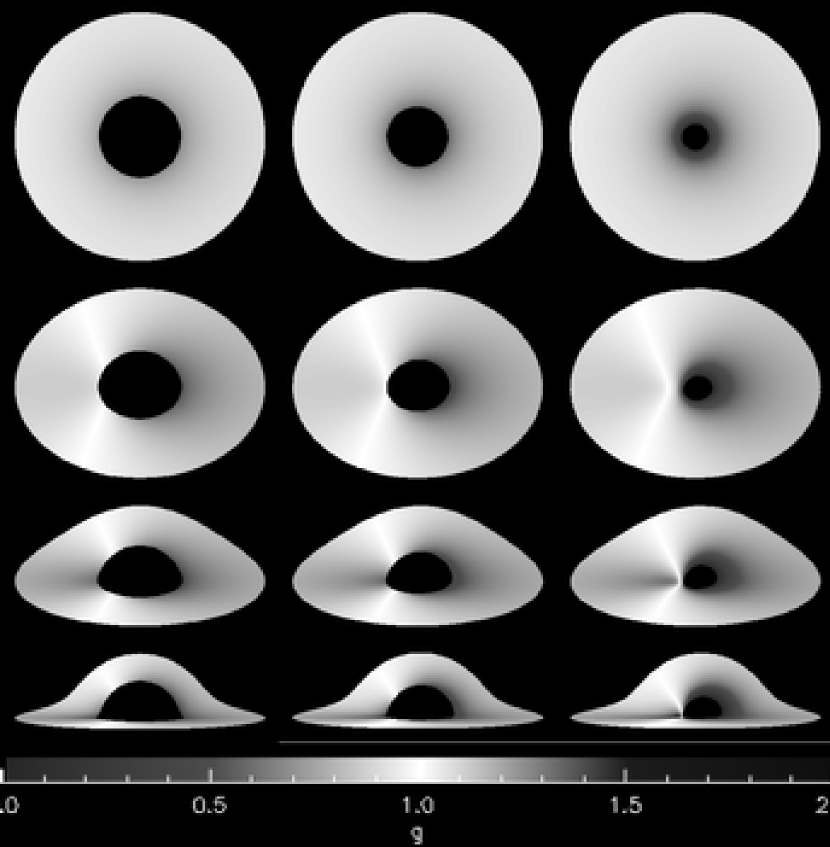
Figure 1: Red-shift map and overall shape of accretion disks around black holes. $g$ is the ratio between the observed energy of a photon and the energy in the rest frame of the disk. Top to bottom: $\theta=5^{\circ},45^{\circ},70^{\circ},85^{\circ}$, $\theta$ is the inclination angle (the angle between the normal of the disk and the line of sight). Left to right: $a=0.01,0.5,0.998$, where $a$ is the specific angular momentum of the black hole. The white zones stand for the regions with zero red-shift (following Fanton et al.(1997) ). Left-hand side of the disk is approaching the observer and blue-shifted.

Figure 3 shows the overall shape of disks due to Doppler and gravitational effects at a large inclination angle ($85^{\circ}$). The inner radius takes the value of the last stable circular orbit. In the first row, the white circles and ellipses show the last stable orbit. The inner contours are greatly distorted by the focusing effect.

Figure 3 shows the comparison between Shwarzschild black holes and Kerr black holes, which shows clearly additional distortion due to frame-dragging effect. Spin results in a smaller last stable orbit, and the inner contour changes from symmetric for $a=0.01$ to asymmetric for $a=0.998$. Therefore in principle, we can tell a rotating black hole from a non-rotating one from the inner contours of their accrection disks.

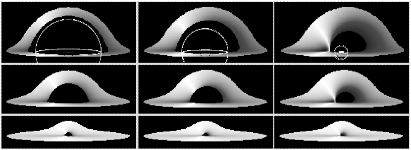
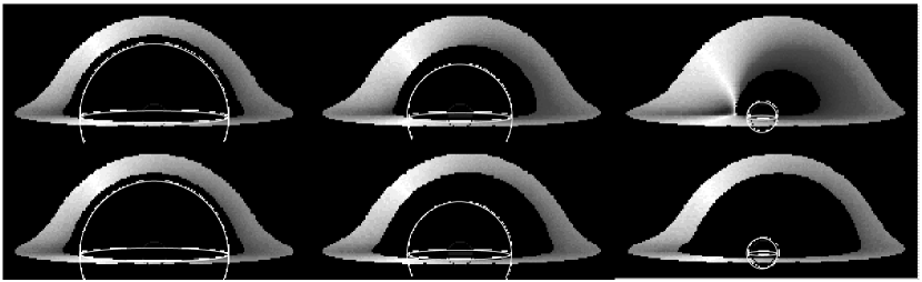
Figure 2: Redshift maps for disks at inclination angle $85^{\circ}$ with different outer radii. Top to bottom: disks with outer radii $10R_{\mathrm{g}}$, $20R_{\mathrm{g}}$, $100R_{\mathrm{g}}$. Left to right: $a=0.01,0.5,0.998$. See text for details.

Figure 3: Redshift maps for 10 $R_{\mathrm{g}}$ disks with different inner radii. Top row: inner radii are the radii of the last stable orbits; Bottom row: inner radii are 6 $R_{\mathrm{g}}$. Left to right: $a=0.01,0.5,0.998$.

2 Images of thin accretion disks

With the redshift map, we calculated images of accretion disks around black holes in several energy ranges. In the calculations, we assume 1) the disks are standard thin disks (Shakura & Sunyaev, 1973); and 2) local radiation results from gravitational potential energy release through blackbody radiation (Page & Thorne 1974). The inner disk radii are the respective last stable orbits.

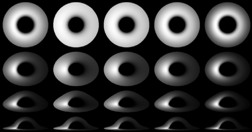
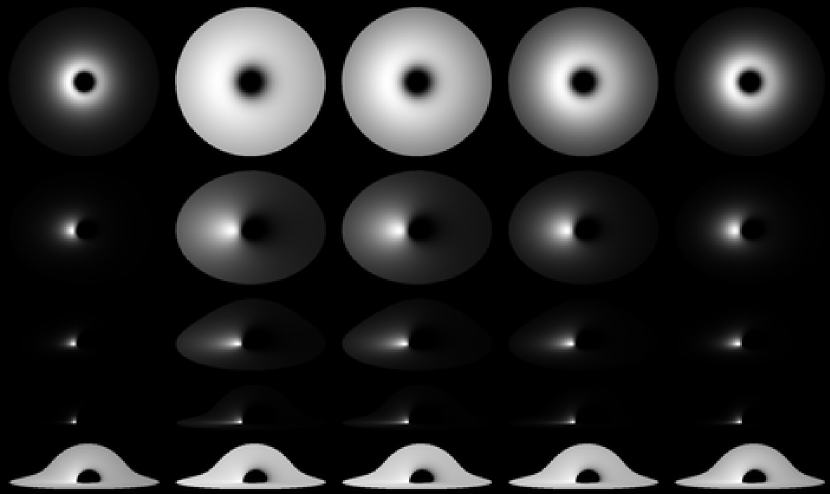
a) $a=0.01$ c) $a=0.998$

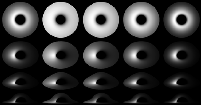
b) $a=0.5$

Figure 4: Disk images of $20R_{\mathrm{g}}$ disks for different spin of the black holes, viewing in certain energy ranges. In all figures, same energy range in a column, and same inclination angle in a row. Left to right: 0.01–100, 0.1–1, 1–2, 2–5, 5–10. Top to bottom: $\theta=5^{\circ},45^{\circ},70^{\circ},85^{\circ},85^{\circ}$. The last image row of c) is the same as the row above it, expect that it is in log scale. c) also shows the scale bar.

In all the images, energy ranges are in the unit of the energy corresponding to the maximum temperature in a non-rotating black hole case. For example, if the maximum temperature in a non-rotating black hole case is 1 keV, then the above energy ranges are 0.1 to 1 keV, 1 to 2 keV etc.. The maximum temperature in the extremal Kerr black hole case is about 5 keV. The images show the brightness in gray scale, with energy flux linearly (if not otherwise specified) mapped to the [0,1] shown on the scale bar in Figure 4c.

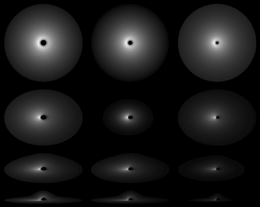
Figure 5: Disk images for $100R_{\mathrm{g}}$ disks in the energy range 0.5 – 2. Top to bottom: $\theta=5^{\circ},45^{\circ},70^{\circ},85^{\circ}$. Left to right: $a=0.01,0.5,0.998$ respectively. 0.5 to 2 keV is the energy range of NASA’s next generation mission MAXIM (Micro-Arcsecond X-ray Imaging Mission) pathfinder. (The images in this figure have a lower contrast than the other images.)

3 Summary and discussion

We studied the images of standard thin accretion disks around black holes under the strong relativistic effects. The expected images for systems with different black hole spin, viewing from different viewing angles and in different energy bands are given. The spin of the black hole not only determines how close the disk can extend to the center, but also causes additional distortion due to the dragging of the frame.

The secondary image are left out because in most cases it will be blocked by the disk, though it might be important in some cases.

Acknowledgments

The authors would like to thank Dr. Fanton for providing us his code of calculating the redshift map and line profile of a thin disk. This study is supported in part by NASA’s Marshall Space Flight Center and through NASA’s Long Term Space Astrophysics Program.

1

References

- [1] Cadez, A., C. Fanton, and M. Calvani, M. (1998). New Astronomy, 3, (No. 8), 647
- [2] Fanton, Claudio, Massimo Calvani, Fernando de Felice, and Andrej Cadez. (1997). PASJ, 49, 159
- [3] Luminet, J.-P.. (1978). A&A, 75, 228
- [4] Page, D.N. & K.S. Thorne. 1974. ApJ, 191, 499
- [5] Shakura, N. I. & Sunyaev, R. A.. 1973. A&A, 24, 337 \chapbblnamechapbib \chapbibliographylogic