Magnetic fields in AGNs and microquasars

Abstract

Observations of AGNs and microquasars by ASCA, RXTE, Chandra and XMM-Newton indicate the existence of wide X-ray emission lines of heavy ionized elements in their spectra. The emission can arise in the inner parts of accretion discs where the effects of General Relativity (GR) must be counted, moreover such effects can dominate. We describe a procedure to estimate an upper limit of the magnetic fields in the regions where X-ray photons are emitted. We simulate typical profiles of the iron $K_{\alpha}$ line in the presence of a magnetic field and compare them with observational data. As an illustration we find $H<10^{10}-10^{11}$ Gs for Seyfert galaxy MCG–6–30–15. Using the perspective facilities of measurement devices (e.g. Constellation-X mission) a better resolution of the blue peak structure of iron $K_{\alpha}$ line will allow to find the value of the magnetic fields if the latter are high enough.

1 Introduction

Recent ASCA, RXTE, Chandra and XMM-Newton observations of Seyfert galaxies demonstrated the existence of the wide iron $K_{\alpha}$ line (6.4 keV) in their spectra along with a number of other weaker lines (Ne X, Si XIII,XIV, S XIV-XVI, Ar XVII,XVIII, Ca XIX, etc.) (see for example, Fabian et al. (1995); Tanaka et al. (1995); Nandra et al. (1997a, b); Malizia et al. (1997); Sambruna et al. (1998); Yaqoob et al. (2001b); Ogle et al. (2000)).

Magnetic fields play a key role in dynamics of accretion discs and jet formation. Bisnovatyi-Kogan & Ruzmaikin (1974, 1976) considered a scenario to generate superstrong magnetic fields near black holes. According to their results magnetic fields near the marginally stable orbit could be about $H\sim 10^{10}-10^{11}$ Gs. Kardashev (1995, 2001a, 2001b, 2001c) considered a generation of synchrotron radiation, acceleration of $e^{+/-}$ pairs and cosmic rays in magnetospheres of supermassive black holes. It is magnetic field, which plays a key role in these models. Below, based on the analysis of iron $K_{\alpha}$ line profile in the presence of a strong magnetic field, we describe how to detect the field itself or at least obtain an upper limit of the magnetic field.

For cases when the spectral resolution is good enough the emission spectral line demonstrates typical two-peak profile with the high ”blue” peak, the low ”red” peak and the long ”red” wing which drops gradually to the background level (Tanaka et al. (1995); Yaqoob et al. (1997)). The Doppler line width corresponds to the velocity of the matter motion of tens of thousands kilometers per second , e.g. the maximum value is about $v\approx 80000-100000$ km/s for the galaxy MCG–6–30–15 (Tanaka et al. (1995); Fabian et al. (2002)) and $v\approx 48000$ km/s for MCG–5–23–16 (Weawer et al. (1998)). For both galaxies the line profiles are known rather well. Fabian et al. (2002) analyzed results of long-time observations of MCG-6-30-15 galaxy using XMM-Newton and BeppoSAX. The long monitoring confirmed the qualitative conclusions about the features of the Fe $K_{\alpha}$ line, which were discovered by ASCA satellite. Yaqoob et al. (2002) discussed the essential importance of ASCA calibrating and the reliability of obtained results. Lee et al. (2002) compared ASCA results with RXTE and Chandra observations for the MCG-6-30-15. Iwasawa et al. (1999); Lee et al. (1999); Shih et al. (2002) analyzed in detail the variability in continuum and in Fe $K_{\alpha}$ line for the MCG-6-30-15 galaxy.

The phenomena of the broad emission lines are supposed to be related with accreting matter around black holes. Wilms et al. (2001); Ballantyne & Fabian (2001); Martocchia et al. (2002b) proposed physical models of accretion discs for the MCG-6-30-15 galaxy and their influence on the Fe $K_{\alpha}$ line shape. Boller et al. (2001) found the features of the spectral line near 7 keV in Seyfert galaxies using data from XMM-Newton satellite. Yaqoob et al. (2001a) presented results of Chandra HETG observations of Seyfert I galaxies.  Qingjuan & Youjun (2001) discussed possible identification of binary massive black holes analyzing Fe $K_{\alpha}$ shape. Ballantyne et al. (2002) estimated abundance of the iron using the data of X-ray observations. Popovic et al. (2001, 2002) discussed an influence of microlensing on the distortion of spectral lines including Fe $K_{\alpha}$ line, that can be significant in some cases. Matt (2002) analyzed an influence of Compton effect on the Fe $K_{\alpha}$ shape for emitted and reflected spectra. Morales & Fabian (2001) proposed a procedure to estimate the masses for supermassive black holes. Fabian (1999) presented a possible scenario for evolution of such supermassive black holes.

A general status of black holes is described in a number of papers (see, e.g. Liang (1998) and references therein, Zakharov (2000); Novikov & Frolov (2001)). Since the matter motions indicate very high rotational velocities, one can assume the $K_{\alpha}$ line emission arises in the inner regions of accretion discs at distances $\sim(1\div 3)~{}r_{g}$ from the black holes. Let us recall that the innermost stable circular for non-rotational black hole (which has the Schwarzschild metric) is located at the distance $3\,r_{g}$ from the black hole singularity. Therefore, a rotation of black hole could be the most essential factor. A possibility to observe the matter motion in so strong gravitational fields could give a chance not only to check general relativity predictions and simulate physical conditions in accretion discs, but investigate also observational manifestations of such astrophysical phenomena like jets (Romanova et al., 1998; Lovelace et al., 1998), some instabilities like Rossby waves (Lovelace et al., 1999) and gravitational radiation.

Wide spectral lines are considered to be formed by radiation emitted in the vicinity of black holes. If there are strong magnetic fields near black holes these lines are split by the field into several components. This phenomenon is discussed below. Such lines have been found in microquasars, GRBs and other similar objects (Balucinska-Church & Church, 1999; Greiner, 1999; Mirabel, 2000, 2002; Lazzati et al., 2001; Martocchia et al., 2002a; Mirabel & Rodriguez, 2002; Miller et al., 2002; Zamanov & Marziani, 2002).

Observations and theoretical interpretations of wide X-ray lines (particularly, the iron $K_{\alpha}$ line) in AGNs are actively discussed in a number of papers (Yaqoob et al., 1996; Wanders et al., 1997; Sulentic et al., 1998a, b; Paul et al., 1998; Bianchi & Matt, 2002; Turner et al., 2002; Levenson et al., 2002a, b). The results of numerical simulations in framework of different physical assumptions on the origin of the wide emissive iron $K_{\alpha}$ line in the nuclei of Seyfert galaxies are presented in papers (Paul et al., 1992; Bromley et al., 1997; Pariev & Bromley, 1997, 1998; Cui et al., 1998; Bromley et al., 1998; Pariev et al., 2000; Ma, 2000, 2002; Karas et al., 2001). The results of Fe $K_{\alpha}$ line observations and their possible interpretation are summarized by Fabian et al. (2001).

To obtain an estimation of the magnetic field we simulate the formation of the line profile for different values of magnetic field. As a result we find the minimal $B$ value at which the distortion of the line profile becomes significant. We use here an approach, which is based on numerical simulations of trajectories of the photons emitted by a hot ring moving along a circular geodesics near black hole, described earlier by Zakharov (1993, 1994, 1995); Zakharov & Repin (1999).

2 Magnetic fields in accretion discs

One of the basic problems to understand the physics of quasars and microquasars is the ”central engine” in these systems, in particular, a physical mechanism to accelerate charged particles and generate high energetic electromagnetic radiation near black holes. The construction of such ”central engine” without magnetic fields could hardly ever be possible. On the other hand magnetic fields give a possibility to extract energy from rotational black holes via Penrose process and Blandford – Znajek mechanism, as it was shown in hydrodynamical simulations by Meier, Koide & Uchida (2001); Koide et al. (2002). The Blandford – Znajek process could provide huge energy release in AGNs (for example, for MCG-6-30-15) and microquasars when the magnetic field is strong enough (Wilms et al., 2001).

Physical aspects of generation and evolution of magnetic fields were considered in a set of reviews (e.g. Asseo & Sol (1987); Giovannini (2001)). A number of papers conclude that in the vicinity of the marginally stable orbit the magnetic fields could be high enough (Bisnovatyi-Kogan & Ruzmaikin, 1974, 1976; Krolik, 1999).

Agol & Krolik (1999) considered an influence of magnetic fields on an accretion rate near the marginally stable orbit and hence on the disc structure, they found the appropriate changes of the emitting spectrum and solitary spectral lines. Vietri & Stella (1998) investigated the instabilities of accretion discs when the magnetic fields play an important role.

3 Photon geodesics in the Kerr metric

Many astrophysical processes where large energy release is observed, are supposed to be related with black holes. Since a large fraction of astronomical objects, such as stars and galaxies, exhibits proper rotation, then there are no doubts that the black holes formed in their nuclei, both stellar and supermassive, possess an intrinsic proper rotation. It is known that stationary black holes are described by the Kerr metric which has the following form in geometrical units $(G=c=1)$ and the Boyer–Lindquist coordinates $(t,r,\theta,\phi)$ (Misner et al., 1973; Landau & Lifshits, 1975):

$$ds^{2}=-\left(1-\frac{2Mr}{\rho^{2}}\right)dt^{2}+\frac{\rho^{2}}{\Delta}dr^{2}+\rho^{2}d\theta^{2}+$$

$$\left(r^{2}+a^{2}+\frac{2Mra^{2}}{\rho^{2}}\sin^{2}\theta\right)\sin^{2}\theta\,d\phi^{2}-\frac{4Mra}{\rho^{2}}\sin^{2}\theta\,d\phi dt,$$ (1)

where

$$\rho^{2}=r^{2}+a^{2}\cos^{2}\theta,$$

$$\Delta=r^{2}-2Mr+a^{2}.$$

Constants $M$ and $a$ determine the black hole parameters: $M$ is its mass, $a\in(0,M)$ is its specific angular moment.

The particle trajectories can be described by the standard geodesic equations:

$$\frac{d^{2}x^{i}}{d\lambda^{2}}+\Gamma^{i}_{kl}\frac{dx^{k}}{d\lambda}\frac{dx^{l}}{d\lambda}=0,$$ (2)

where $\Gamma^{i}_{kl}$ are the Christoffel symbols and $\lambda$ is the affine parameter. These equations can be simplified if we will use the complete set of the first integrals which were found by Carter (1968): $E=p_{t}$ is the particle energy at infinity, $L_{z}=p_{\phi}$ is the projection of its angular momentum on the rotation axis, $m=(p_{i}p^{i})^{1/2}$ is the particle mass and $Q$ is the Carter separation constant:

$$Q=p_{\theta}^{2}+\cos^{2}\theta\left[a^{2}\left(m^{2}-E^{2}\right)+L_{z}^{2}/\sin^{2}\theta\right].$$ (3)

The equations of photon motion ($m=0$) can be reduced to the following system of ordinary differential equations (Zakharov, 1991, 1994):

$$\frac{dt}{d\sigma} = -a\left(a\sin^{2}\theta-\xi\right)+\frac{r^{2}+a^{2}}{\Delta}\left(r^{2}+a^{2}-\xi a\right),$$ (4)

$$\frac{dr}{d\sigma} = r_{1},$$ (5)

$$\frac{dr_{1}}{d\sigma} = 2r^{3}+\left(a^{2}-\xi^{2}-\eta\right)r+\left(a-\xi\right)^{2}+\eta,$$ (6)

$$\frac{d\theta}{d\sigma} = \theta_{1},$$ (7)

$$\frac{d\theta_{1}}{d\sigma} = \cos\theta\left(\frac{\xi^{2}}{\sin^{3}\theta}-a^{2}\sin\theta\right),$$ (8)

$$\frac{d\phi}{d\sigma} = -\left(a-\frac{\xi}{\sin^{2}\theta}\right)+\frac{a}{\Delta}\left(r^{2}+a^{2}-\xi a\right),$$ (9)

where $\sigma$ is an independent variable, $\eta=Q/M^{2}E^{2}$ and $\xi=L_{z}/ME$ are the Chandrasekhar’s constants (Chandrasekhar, 1983) which should be derived from initial conditions in the disc plane; $t$, $r$ and $a$ are here the appropriate dimensionless variables (in the mass units). The system (4)-(9) has two first integrals,

$$\epsilon_{1} \equiv r_{1}^{2}-r^{4}-\left(a^{2}-\xi^{2}-\eta\right)r^{2}-$$ (10)

$$\phantom{.}-2\left[\left(a-\xi\right)^{2}+\eta\right]r+a^{2}\eta=0,$$

$$\epsilon_{2} \equiv \theta_{1}^{2}-\eta-\cos^{2}\theta\left(a^{2}-\frac{\xi^{2}}{\sin^{2}\theta}\right)=0,$$ (11)

which can be used for the accuracy control of computation.

The additional variables $r_{1}$ and $\theta_{1}$ reduce the Eqs. (5)–(8) to a non-singular form. Such kind representation allows to avoid the integration difficulties which usually appears when the equations are written in standard form (Misner et al., 1973; Landau & Lifshits, 1975) for $r$ and $\theta$ coordinates.

A qualitative analysis of the geodesic equations showed that types of photon motion can drastically change with small changes of chosen geodesic parameters (Zakharov, 1986, 1989). Therefore, the standard way where there is one equation for each Boyer-Lindquist coordinate (reducing to calculation of the elliptical integrals) can lead to large numerical errors (Zakharov, 1991). The integration of Eqs. (4)–(9) allows to avoid such problem and realizes this process without essential numerical errors.

Solving Eqs. (4)–(9) for monochromatic quanta emitted by a hot ring rotating on circular geodesics at radius $r$ in the equatorial plane, we can obtain the ring spectrum $I_{\nu}(r,\theta_{\infty})$ which is registered by a distant observer in the position characterized by the angle $\theta_{\infty}=\theta\big{|}_{r=\infty}$. The numerical integration is performed using the Gear and Adams methods  (Gear, 1971) and the standard package realized by Hindmarsh (1983); Petzold (1983); Hiebert & Shampine (1983). We obtain the entire disc spectrum by summation of sharp ring spectra.

4 Disc radiation model

To simulate the radiated spectrum it is necessary first to adopt some emission model. We assume that the source of the emitting quanta is a narrow and thin disc (ring) rotating in the equatorial plane of a Kerr black hole. For $a=0.01$ the marginally stable orbit lies at $r_{ms}=2.9836\,r_{g}$, the difference from $3\,r_{g}$ ($r_{g}=2M$) is not important for our analysis. We also assume that disc is opaque to radiation, so that a distant observer situated on one disc side cannot register the quanta emitted fron its another side.

For the sake of computational simplicity we suggest that the spectral line is monochromatic in its co-moving frame. To approve this assumption one can argue that even at $T=10^{8}$ K the thermal width of the line

$$\frac{\delta f}{f}\sim\frac{1}{c}\sqrt{\frac{kT}{m_{{}_{\rm Fe}}}}\approx 10^{-3}$$

appears to be much less than the Doppler line width associated with the disc rotation.

Note that we do not assume any particular model of the accreting disc. As an illustration we determine the dependence of disc temperature on the radial coordinate according to the standard $\alpha$-disc model (Shakura & Sunyaev, 1973; Shakura, 1973; Lipunova & Shakura, 2002). The radiation intensity is, as usually, proportional to $T^{4}$.

The emission intensity of the ring at a given radius $r$ is proportional to the area of the ring. The area of emitting ring of the width $dr$ differs in the Schwarzschild metric from its classical expression $dS=2\pi rdr$ and should be replaced with

$$dS=\frac{2\pi r\,dr}{\displaystyle\sqrt{1-\frac{r_{g}}{r}\phantom{1}}}.$$ (12)

Thus, the total flux density emitted by the disc and registered by distant observer is proportional to the integral

$$J_{\nu}(\theta_{\infty})=\int\limits_{r_{in}}^{r_{out}}I_{\nu}(r,\theta_{\infty})T^{4}(r)dS,$$ (13)

where $J_{\nu}(r,\theta_{\infty})$ is obtained from the solution of equations (4)–(9), $T(r)$ – from the appropriate dependence for $\alpha$-disc and $dS$ – from Eq. (12).

The radiation pressure predominates in the innermost part of the disc ($a$) while the gas pressure – in the middle ($b$). The boundary $r_{ab}$ between these two regions can be found for $\alpha$-disc from the following equation (Shakura & Sunyaev, 1973)

$$\frac{r_{ab}/(3r_{g})}{\left(1-\sqrt{3r_{g}/r_{ab}}\right)^{16/21}}=150(\alpha M/M_{\odot})^{2/21}\dot{m}^{16/21},$$ (14)

which we solve by an iteration procedure. In Eq.(14) we have $\dot{m}=\dot{M}/\dot{M}_{cr}$, where $\dot{M}_{cr}=3\cdot 10^{-8}M$/yr. Thus, for $\alpha=0.2$, $M=10^{8}M_{\odot}$ and $\dot{m}=0.1$ we have from Eq.(14) $r_{ab}\approx 360\,r_{g}$.

For simulation we assume that the emitting region lies as whole in the innermost region of the disc (zone $a$). If this condition is not satisfied, the profile of a spectral line becomes extremely complicated, so that it appears difficult to avoid the uncertainty in interpretation. Thus, we assume that emission arises in the region from $r_{out}=10\,r_{g}$ to $r_{in}=3\,r_{g}$ and the emission is monochromatic in the co-moving frame. Set the frequency of this emission as a unity by convention.

5 Influence of a magnetic field on the distortion of the iron $K_{\alpha}$ line profile

The magnetic pressure at the inner edges of the accretion discs and its correspondence with parameter $a$ in the frameworks of disc accretion models is discussed by Krolik (2001). However, the numerical value of magnetic field is determined there from a model-dependent procedure, a number of parameters in which cannot be found explicitly from observations.

Here we consider the influence of a magnetic field on the iron $K_{\alpha}$ line profile and show how one can determine the value of the magnetic field strength or at least an upper limit.

The profile of a monochromatic line (Zakharov & Repin, 1999, 2002a, 2002b) depends on the angular momentum of a black hole, the position angle between the black hole axis and the distant observer position, the value of the radial coordinate if the emitting region represents an infinitesimal ring (or two radial coordinates for outer and inner bounds of a wide disc).

We assume that the emitting region is located in an area of strong quasi-static magnetic field. This field causes line splitting due to the standard Zeeman effect. There are three characteristic frequencies of the split line that arise in the emission. The energy of central component $E_{0}$ remains unchanged, whereas two extra components are shifted by $\pm\mu_{B}H$, where $\mu_{B}=\dfrac{e\hbar}{2m_{\rm e}c}=9.273\cdot 10^{-21}$ erg/Gs is the Bohr magneton. Therefore, in the presence of a magnetic field we have three energy levels: $E_{0}-\mu_{B}H,~{}E_{0}$ and $E_{0}+\mu_{B}H$. For the iron $K_{\alpha}$ line they are as follows: $E_{0}=6.4-0.58\dfrac{H}{10^{11}\,{\rm Gs}}$ keV, $E_{0}=6.4$ keV and $E_{0}=6.4+0.58\dfrac{H}{10^{11}\,{\rm Gs}}$ keV.

Let us discuss how the line profile changes when photons are emitted in the co-moving frame with energy $E_{0}(1+\epsilon)$, but not with $E_{0}$. In that case the line profile can be obtained from the original one by $1+\epsilon$ times stretching along the x-axis which counts the energy. The component with $E_{0}(1-\epsilon)$ energy should be $(1-\epsilon)$ times stretched, respectively. The intensity of different Zeeman components are approximately equal (Fock, 1976). A composite line profile can be found by summation the initial line with energy $E_{0}$ and two other profiles, obtained by stretching this line along the $x$-axis in $(1+\epsilon)$ and $(1-\epsilon)$ times correspondingly. The line intensity depends on the direction of the quantum escape with respect to the direction of the magnetic field (Berestetskii et al., 1982). However, we neglect this weak dependence (undoubtedly, the dependence can be counted and, as a result, some details in the spectrum profile can be slightly changed, but the qualitative picture, which we discuss, remains unchanged).

Figure 1: Profile of monochromatic spectral line, emitted by $\alpha$-disc in Schwarzschild metric for $r_{out}=10\,r_{g}$, $r_{in}=3\,r_{g}$ and inclination angles $\theta=60^{\circ}$ (top panel) and $\theta=50^{\circ}$ (bottom panel) with zero value of magnetic field. The line profile shown as it is registered by a distant observer.

Figure 2: Distortions of the line profile from the top panel in Fig. 1, arising due to a quasi-static magnetic field existing in the disc. The Zeeman effect leads to the appearance of two extra components with the energies higher and lower than the basic one. The values of the magnetic field are shown at each panel.

Another indicator of the Zeeman effect is a significant induction of the polarization of X-ray emission: the extra lines possess a circular polarization (right and left, respectively, when they are observed along the field direction) whereas a linear polarization arises if the magnetic field is perpendicular to the line of sight. Despite of the fact that the measurements of polarization of X-ray emission have not been carried out yet, such experiments can be realized in the nearest future (Costa et al., 2001).

Figure 3: The same as in Fig. 2, but for $\theta=50\degr$. The bottom panel on Fig. 1 demonstrates the same spectrum without magnetic field.

Figure 4: The same as in Fig. 3, but for minimum value of magnetic field at which it is possible to observe the splitting of the line.

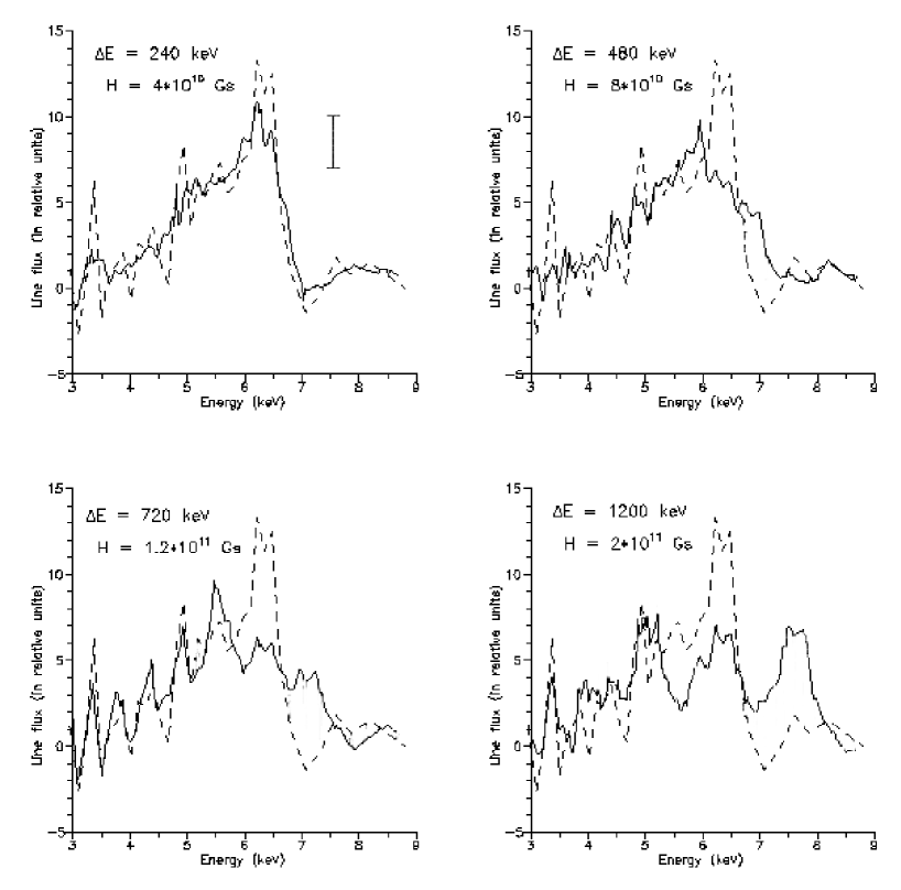
Figure 5: Influence of a magnetic field on the observational data. The dashed line represents the ASCA observations of MCG-6-30-15 (Tanaka et al., 1995). The vertical bar in the top left panel corresponds to a typical error in observation data. Solid lines show possible profiles of $K_{\alpha}$ line in a presence of a magnetic field. The field value and the appropriate Zeeman splitting are indicated in each panel.

The line profile without any magnetic field is presented in Fig. 1 for different values of disc inclination angles: $\theta=60^{\circ}$ and $\theta=50^{\circ}$ respectively. Note, than at $\theta=50^{\circ}$ the blue peak appears more tall and narrow. Figs. 2,3 present the line profiles for the same inclination angles and different values of magnetic field: $H=4\cdot 10^{10}$, $8\cdot 10^{10}$, $1.2\cdot 10^{11}$, $2\cdot 10^{11}$ Gs. At $H=4\cdot 10^{10}$ Gs the shape of spectral line does not practically differ from the one with zero magnetic field. Three components of the blue peak are so thin and narrow that they could be scarcely distinguished experimentally today. For $H<4\cdot 10^{10}$ Gs and $\theta=60\degr$ the splitting of the line does not arise at all. At $\theta=50\degr$ the splitting can still be revealed for $H=3\cdot 10^{10}$ Gs (see Fig. 4), but below this value ($H<3\cdot 10^{10}$ Gs) it also disappears. With increasing the field the splitting becomes more explicit, and at $H=8\cdot 10^{10}$ Gs a faint hope appears to register experimentally the complex internal structure of the blue maximum.

While further increasing the magnetic field the peak profile structure becomes apparent and can be distinctly revealed, however, the field $H=2\cdot 10^{11}$ Gs is rather strong, so that the classical linear expression for the Zeeman splitting

$$\Delta E=\pm\mu_{B}H$$ (15)

should be modified. Nevertheless, we use Eq.(15) for any value of the magnetic field, assuming that the qualitative picture of peak splitting remains correct, whereas for $H=2\cdot 10^{11}$ Gs the exact maximum positions may appear slightly different. If the Zeeman energy splitting $\Delta E$ becomes of the order of $E$, the line splitting due to magnetic fields is described in a more complicated way. The discussion of this phenomenon is not a point of this paper, our goal is to pay attention to the qualitative features of this effect.

Fig. 5 demonstrates a possible influence of the Zeeman effect on observational data. As an illustration we consider the observations of iron $K_{\alpha}$ line which have been carried out by ASCA for the galaxy MCG-6-30-15. They are presented in Fig. 5 in the dashed curve. Let us assume that the actual magnetic field in these data is negligible. Then we can simulate the influence of the Zeeman effect on the structure of observations and see if the simulated data (with a magnetic field) can be distinguishable within the current accuracy of the observations. The results of the simulated observation for the different values of magnetic field are shown in Fig. 5 in solid line. From these figures one can see that classical Zeeman splitting in three components, which can be revealed experimentally today, changes qualitatively the line profiles only for rather high magnetic field. Something like this structure can be detected, e.g. for $H=1.2\cdot 10^{11}$ Gs, but the reliable recognition of three peaks here is hardly possible.

Apparently, it would be more correctly to solve the inverse problem: to try to determine the magnetic field in the disc, assuming that the blue maximum is already split due to the Zeeman effect. However, this problem includes too many additional factors, which can affect on the interpretation. Thus, beside of magnetic field the line width depends on the accretion disc model as well as on the structure of emitting regions. Such kind problems may become actual with a much better accuracy of observational data in comparison with their current state.

6 Discussion

It is evident that the cause of duplication (triplication) of a blue peak could be not only the influence of a magnetic field (the Zeeman effect), but a number of other factors. For example, the line profile can have two peaks when the emitting region represents two narrow rings with different values of radial coordinate (it is easy to conclude that two emitting rings with finite widths separated by a gap, would yield a similar effect). Despite of the fact that a multiple blue peak can originate from many causes (including the Zeeman effect as one of possible explanation), the absence of the multiple peak can result in the conclusion about the upper limit of the magnetic field.

It is known that neutron stars (pulsars) could have huge magnetic fields. So, it means that the discussed above effect could appear in binary neutron star systems. The quantitative description, however, needs more detailed computations for such systems.

With further increasing of observational facilities it may become possible to improve the above estimation. Thus, the Constellation-X launch suggested in the coming decade seems to increase the precision of X-ray spectroscopy as many as approximately 100 times with respect to the present day measurements (Weawer, 2001). Therefore, there is a possibility in principle that the upper limit of the magnetic field can also be 100 times improved in the case when the emission of the X-ray line arise in a sufficiently narrow region.

7 Acknowledgements

One author (A.F.Z.) is grateful to E.F.Zakharova for kindness and support, necessary to complete this work.

S.V.R. is very grateful to Prof. E.V.Starostenko, Dr. A.M.Salpagarov, Dr. O.N.Sumenkova and L.V.Bankalyuk for the possibility of successful and intensive work over the problem.

The authors are grateful to E.A.Dorofeev, S.V.Molodtsov, L.Popovic and A.I.Studenikin for useful discussion.

This work has been partly supported by Russian Foundation for Basic Research (grants 00–02–16108 (AFZ & SVR), 01-02-16274 (VNL)) and the State Program in Astronomy (NSK).

References

- Agol & Krolik (1999) Agol E., Krolik J.H., 2000, ApJ, 528, 161 (astro-ph/9908049).
- Asseo & Sol (1987) Asseo E., Sol H., 1987, Physics Reports, 148, 307.
- Ballantyne & Fabian (2001) Ballantyne D.R., Fabian A.C., 2001, MNRAS, 328, L11 (astro-ph/0104342).
- Ballantyne et al. (2002) Ballantyne D.R., Fabian A.C., Ross R.R., 2002, MNRAS, 329, L67 (astro-ph/0112179).
- Balucinska-Church & Church (1999) Balucinska-Church M., Church M.J., 2000, MNRAS, 312, L55 (astro-ph/9912389).
- Berestetskii et al. (1982) Berestetskii V.B., Lifshits E.M., Pitaevskii L.P., 1982, Quantum electrodynamics, Pergamon Press, Oxford.
- Bianchi & Matt (2002) Bianchi S., Matt G., 2002, A&A, 387, 76.
- Bisnovatyi-Kogan & Ruzmaikin (1974) Bisnovatyi-Kogan G.S., Ruzmaikin A.A., 1974, A&SS, 28, 45.
- Bisnovatyi-Kogan & Ruzmaikin (1976) Bisnovatyi-Kogan G.S., Ruzmaikin A.A., 1976, A&SS, 42, 401.
- Blokhintsev (1963) Blokhintsev D.I., 1964, Quantum mechanics, D. Reidel Publ. Co. Dordrecht, Holland.
- Boller et al. (2001) Boller Th., Fabian A.C., Sunyaev R. et al., 2002, MNRAS, 329, L1 (astro-ph/0110367).
- Bromley et al. (1997) Bromley B.C., Chen K., Miller W.A., 1997, ApJ, 475, 57.
- Bromley et al. (1998) Bromley B.C., Miller W.A., Pariev V.I., 1998, Nature, 391, 54.
- Carter (1968) Carter B., 1968, Phys.Rev. D, 174, 1559.
- Chandrasekhar (1983) Chandrasekhar S., 1983, Mathematical Theory of Black Holes, Clarendon Press, Oxford.
- Costa et al. (2001) Costa E., Soffitta P., Belazzini R. et al., 2001, Nature, 411, 662.
- Cui et al. (1998) Cui W., Zhang S.N., Chen W., 1998, ApJ, 257, 63.
- Dirac (1960) Dirac P.A.M., 1958, The principles of quantum mechanics, 4-th Edition, Oxford University Press.
- Fabian et al. (1995) Fabian A.C., Nandra K., Reynolds C.S. et al., 1995, MNRAS, 277, L11.
- Fabian (1999) Fabian A.C., 1999, MNRAS, 308, L39 (astro-ph/9908064).
- Fabian et al. (2001) Fabian A.C., 2001, in Relativistic Astropysics, Texas Symposium, American Institute of Physics, AIP Conference Proceedings, 586, 643.
- Fabian et al. (2002) Fabian A.C., Vaughan S., Nandra K., accepted to MNRAS (astro-ph/0206095).
- Fock (1976) Fock V.A., 1978, Fundamentals of quantum mechanics, Mir, Moscow.
- Gear (1971) Gear C.W., 1971, Numerical Initial Value Problems in Ordinary Differential Equations. Prentice Hall, Englewood Cliffs, NY.
- Giovannini (2001) Giovannini M., hep-ph/0111220.
- Greiner (1999) Greiner J., 2000, in ”Cosmic Explosions”, Proceedings of 10th Annual Astrophysical Conference in Maryland, eds. S.Holt & W.W.Zang, AIP Conference proceedings, 522, 307 (astro-ph/9912326).
- Hiebert & Shampine (1983) Hiebert K.L., Shampine L.F., 1980, Implicitly Defined Output Points for Solutions of ODE-s. Sandia report sand80–0180, February.
- Hindmarsh (1983) Hindmarsh A.C., in Stepleman, R.S. et al. eds, ODEpack, a systematized collection of ODE solvers. In Scientific Computing, North–Holland, Amsterdam, p. 55.
- Iwasawa et al. (1999) Iwasawa K., Fabian A.C., Young A.J. et al., 1999, MNRAS, 306, L19 (astro-ph/9904078).
- Karas et al. (2001) Karas V., Martocchia A., Subr L., 2001, PASJ, 53, 189 (astro-ph/0102460).
- Kardashev (1995) Kardashev N.S., 1995, MNRAS, 276, 515.
- Kardashev (2001a) Kardashev N.S., 2001a, in Giancarlo Setti and Jean-Pierre Swings eds., Quasars, AGNs and Related Research Across 2000. Conference on the occasion of L.Woltjer’s 70th birthday, Rome, Italy, May 2000. Springer, p.66.
- Kardashev (2001b) Kardashev N.S., 2001b, in Kardashev N.S., Dagkesamanskij R.D., Kovalev Yu.A. eds, Astrophysics on the edge of centuries. Proceedings of Russian astronomical conference, Pushchino. Yanus-K, Moscow, p. 383.
- Kardashev (2001c) Kardashev N.S., 2001c, MNRAS, 326, 1122.
- Koide et al. (2002) Koide S., Shibata K., Kudoh T. et al., 2002, Science, 295, 1688.
- Krolik (1999) Krolik J.H., 1999, ApJ, 515, L73 (astro-ph/9902267).
- Krolik (2001) Krolik J.H., 2001, in Relativistic Astropysics, Texas Symposium, American Institute of Physics, AIP Conference Proceedings, 586, p. 674.
- Landau & Lifshits (1975) Landau L.D., Lifshits E.M., The classical theory of fields, 1975, Pergamon Press, Oxford.
- Lazzati et al. (2001) Lazzati D., Ghisellini G., Vietri M. et al., 2001, in Enrico Costa, Filippo Frontera, Jens Hjorth eds, Proceedings of the International workshop held in Rome, CNR headquaters. Springer, Berlin Heidelberg, p. 236 (astro-ph/0104086).
- Lee et al. (1999) Lee J.C., Fabian A.C., Reynolds C.S. et al., 2000, MNRAS, 318, 857 (astro-ph/9909239).
- Lee et al. (2002) Lee J.C., Iwasawa K., Houck J.C. et al., 2002, ApJ, 570, L47 (astro-ph/0203523).
- Levenson et al. (2002a) Levenson N.A. et al., 2002, ApJ, 573, L84.
- Levenson et al. (2002b) Levenson N.A., Krolik J.H., Zycki P.T. et al., 2002, ApJ, 573, L81 (astro-ph/0206071).
- Liang (1998) Liang E.P., 1998, Physics Reports, 302, 69.
- Lipunova & Shakura (2002) Lipunova G.V., Shakura N.I., 2002, Astronomy Reports, 46, 366.
- Lovelace et al. (1998) Lovelace R.V.E., Newman W.I., Romanova M.M., 1997, ApJ, 484, 628.
- Lovelace et al. (1999) Lovelace R.V.E., Li H., Colgate S.A. et al., 1999, ApJ, 513, 805.
- Malizia et al. (1997) Malizia A., Bassani L., Stephen J.B. et al., 1997, ApJSS, 113, 311.
- Martocchia et al. (2002a) Martocchia A., Matt G., Karas V. et al., 2002, A&A, 387, 215 (astro-ph/0203185).
- Ma (2000) Ma Zhen-guo, 2000, Chinese A&A, 24, 135.
- Ma (2002) Ma Zhen-guo, 2002, in Proc. IAU 214 Symposium (in press).
- Martocchia et al. (2002b) Martocchia A., Matt G., Karas V., 2002, A&A, 383, L23 (astro-ph/0201192).
- Paul et al. (1992) Matt G., Perola G.C., Piro L., Stella L., 1992, A&A, 475, 57.
- Matt (2002) Matt G., accepted in MNRAS (astro-ph/0207615).
- Meier, Koide & Uchida (2001) Meier D.L., Koide S., Uchida Y., 2001, Science, 291, 84.
- Messia (1976) Messia A., 1976, Quantenmechanik, Walter de Geuter, Berlin.
- Miller et al. (2002) Miller J.M., Fabian A.C., Wijnands R. et al., 2002, ApJ, 570, L73.
- Mirabel (2000) Mirabel I.F, 2001, A&SSS, 276, 319 (astro-ph/0011315).
- Mirabel (2002) Mirabel I.F, 2002, private communication.
- Mirabel & Rodriguez (2002) Mirabel I.F, Rodriguez L.F., 2002, Sky & Telescope, May, 33.
- Misner et al. (1973) Misner C.W., Thorne K.S., Wheeler J.A., 1973, Gravitation. W.H.Freeman, San Francisco.
- Morales & Fabian (2001) Morales R., Fabian A.C., 2002, MNRAS, 329, 209 (astro-ph/0109050).
- Nandra et al. (1997a) Nandra K., George I.M., Mushotzky R.F. et al., 1997, ApJ, 476, 70.
- Nandra et al. (1997b) Nandra K., George I.M., Mushotzky R.F. et al., 1997, ApJ, 477, 602.
- Novikov & Frolov (2001) Novikov I.D., Frolov V.P., 2001, Physics – Uspekhi, 44, 291.
- Novikov & Thorne (1973) Novikov I.D., Thorne K.S., 1973, in De Witt C., De Witt B.S. eds, Black Holes. New York: Gordon & Breach, p. 334.
- Ogle et al. (2000) Ogle, P.M., Marshall, H.L., Lee J.C. et al., 2000, ApJ, 545, L81.
- Pariev & Bromley (1997) Pariev V.I, Bromley B.C., 1997, Proceedings of the 8-th Annual October Astrophysics Conference in Maryland (astro-ph/9711214).
- Pariev & Bromley (1998) Pariev V.I., Bromley B.C., 1998, ApJ, 508, 590.
- Pariev et al. (2000) Pariev V.I., Bromley B.C., Miller W.A., 2001, ApJ, 547, 649 (astro-ph/0010318).
- Paul et al. (1998) Paul, B., Agrawal, P.C., Rao, A.R. et al., 1998, ApJ, 492, 15.
- Petzold (1983) Petzold L.R., 1983, SIAM J. Sci. Stat. Comput, 4, 136.
- Popovic et al. (2001) Popović L.C., Mediavilla E.G., Munoz J.A., 2001, A&A, 378, 295.
- Popovic et al. (2002) Popović L.C., Mediavilla E.G., Jovanović P. et al. 2002, accepted
- Qingjuan & Youjun (2001) Qingjuan Yu, Youjun Lu, 2001, A&A, 377, 17.
- Romanova et al. (1998) Romanova M.M., Ustyugova G.V., Koldoba A.V. et al., 1998, ApJ, 500, 703.
- Sambruna et al. (1998) Sambruna R.M., George I.M., Mushotsky R.F. et al., 1998, ApJ, 495, 749.
- Sazonov et al. (2002) Sazonov S.Yu., Churazov E.M., Sunyaev R.A., 2002, MNRAS, 330, 817.
- Shakura (1973) Shakura N.I., 1972, A. Zh., 49, 921.
- Shakura & Sunyaev (1973) Shakura N.I., Sunyaev R.A., 1973, A&A, 24, 337.
- Shih et al. (2002) Shih D.C., Iwasawa K., Fabian A.C., 2002, MNRAS, 2002, 333, 687 (astro-ph/9904078).
- Sulentic et al. (1998b) Sulentic J.W., Marziani P., Zwitter T. et al., 1998, ApJ, 501, 54.
- Sulentic et al. (1998a) Sulentic J.W., Marziani P., Calvani M., 1998, ApJ, 497, L65.
- Tanaka et al. (1995) Tanaka Y., Nandra K., Fabian A.C. et al., 1995, Nature, 375, 659.
- Turner et al. (2002) Turner T. J., Mushotzky R.F., Yagoob T. et al., 2002, ApJ, 574, L127.
- Vietri & Stella (1998) Vietri M., Stella L., 1998, ApJ, 503,350 (astro-ph/9803089).
- Wanders et al. (1997) Wanders I. et al., 1997, ApJSS, 113, 69.
- Weawer et al. (1998) Weawer K.A., Krolik J.H., Pier E.A., 1998, ApJ, 498, 213, (astro-ph/9712035).
- Weawer (2001) Weaver K.A., 2001, in Relativistic Astropysics, Texas Symposium, American Institute of Physics, AIP Conference Proceedings, 586, p. 702.
- Wilms et al. (2001) Wilms J., Reynolds C.S., Begelman M.C. et al. 2001, MNRAS, 328, L27 (astro-ph/0110520).
- Yaqoob et al. (1996) Yaqoob T., Serlemitsos P.J., Turner T.J. et al., 1996, ApJ, 470, L27.
- Yaqoob et al. (1997) Yaqoob T., McKernan B., Ptak A. et al., 1997, ApJ, 490, L25.
- Yaqoob et al. (2001a) Yaqoob T., George I.M., Turner T.J., astro-ph/0111428.
- Yaqoob et al. (2001b) Yaqoob T., George I.M., Nandra, K. et al., 2001, ApJ, 546, 759.
- Yaqoob et al. (2002) Yaqoob T., Padmanabhan U., Dotani T. et al., 2002, ApJ, 569, 487.
- Zakharov (1986) Zakharov A.F., 1986, JEThP, 91, 3.
- Zakharov (1989) Zakharov A.F., 1989, JEThP, 95, 385.
- Zakharov (1991) Zakharov A.F., 1991, Soviet Astronomy, 35, 147.
- Zakharov (1993) Zakharov A.F., 1993, Preprint MPA 755.
- Zakharov (1994) Zakharov A.F., 1994, MNRAS, 269, 283.
- Zakharov (1995) Zakharov A.F., 1995, in Annals for the 17th Texas Symposium on Relativistic Astropysics, The New York Academy of Sciences, 759, 550.
- Zakharov (2000) Zakharov A.F., 2000, in Proc. of the XXIII Workshop on High Energy Physics and Field Theory, IHEP, Protvino, 169.
- Zakharov & Repin (1999) Zakharov A.F., Repin S.V., 1999, Astronomy Reports, 43, 705.
- Zakharov & Repin (2002a) Zakharov A.F., Repin S.V., 2002, Astronomy Reports, 46, 360.
- Zakharov & Repin (2002b) Zakharov A.F., Repin S.V., 2002, in J. Koga, T. Nakamura, K. Maeda, K. Tomita (eds), Proc. of the Eleven Workshop on General Relativity and Gravitation in Japan, Waseda University, Tokyo, p. 68.
- Zamanov & Marziani (2002) Zamanov R., Marziani P., astro-ph/0204423 (accepted in ApJ).