Major Mergers of Haloes, Growth of Massive Black Holes and Evolving Luminosity Function of Quasars

Abstract

We construct a physically motivated analytical model for the quasar luminosity function, based on the joint star formation and feeding of massive black holes suggested by the observed correlation between the black hole mass and the stellar mass of the hosting spheroids. The parallel growth of massive black holes and host galaxies is assumed to be triggered by major mergers of haloes. The halo major merger rate is computed in the frame of the extended Press-Schechter model. The evolution of black holes on cosmological timescales is achieved by the integration of the governing set of differential equations, established from a few reasonable assumptions that account for the distinct (Eddington-limited or supply-limited) accretion regimes. Finally, the typical lightcurves of the reactivated quasars are obtained under the assumption that, in such accretion episodes, the fall of matter onto the black hole is achieved in a self-regulated stationary way. The predicted quasar luminosity function is compared to the luminosity functions of the 2dF QSO sample and other, higher redshift data. We find good agreement in all cases, except for $z<1$ where the basic assumption of our model is likely to break down.

1 INTRODUCTION

In the last decade, a considerable progress has been achieved towards the understanding of the nature and evolution of Active Galactic Nuclei (AGN). It is now commonly accepted that they are powered by Massive Black Holes (MBHs) fuelled by material originating in the hosting dark-matter haloes and infalling from the close galactic environment in the process described as accretion. New models connecting the AGN phenomenon to the hierarchical growth of haloes have been developed, based on increasingly robust theoretical background substituting phenomenology. In this frame, the masses of MBHs are usually assumed to scale with the masses of the hosting dark-matter haloes with density estimated from the Press & Schechter (1974) formalism (e.g. Efstathiou & Rees 1988; Haiman & Loeb 1998). The AGN luminosity is supposed close to the Eddington value during a “duty cycle” that can be as short as $10^{6}$ to some $10^{7}$ years (e.g. Haiman & Loeb 1998; Martini & Weinberg 2001; Wyithe & Loeb 2002) or longer, of the order of some $10^{8}$ years (e.g. Haehnelt & Rees 1993; Haehnelt et al. 1998). With time, these models have become more and more complex and complete. The accretion rate onto the MBH varies depending on the model: it can be constant or redshift-dependent (Kauffmann & Haehnelt 2000; Haiman & Menou 2000). The AGN activity in many cases appears to be a recurrent event (Siemiginowska & Elvis 1997; Hatziminaoglou et al. 2001). The diverging opinions as to this recurrence have converged, accounting for tidal interactions and merging effects. In addition, the Eddington-limited capability of MBHs to accrete mass and the progressive consumption of the hot gas available in haloes are also expected to play an important role in the evolution of AGN luminosities (Cavaliere & Vittorini, 2000).

In several recent papers (1998; Monaco et al. 2000; Granato et al. 2001; Archibald et al. 2002; Volonteri, Haardt & Madau 2003 and references therein), the joint modelling of star formation and the growth of MBHs lying in galactic nuclei has been considered in order to account for the observed correlation between the masses of the MBH and the hosting spheroid (Wandel, 1999; Woo & Urry, 2002). Spheroids grow through galaxy mergers, giving rise to new ellipticals, and through the mass transfer from unstable discs (possibly not even settled down) to bulges. Although none of these processes is directly associated with the Major Merger (MM) of dark-matter haloes, some concatenation of events is believed to correlate both phenomena. Firstly, MMs mark the beginning of the orbital decay, through dynamical friction, of the more massive galaxies of the progenitors, which eventually merge at the center of the new halo. Secondly, the shock-heated gas is redistributed and begins to cool from the central higher density region at the strongest rate ever reached during the whole halo life. Large amounts of gas then fall into the central galaxy making its disc easily become unstable (particularly at high redshifts where discs are more compact) and transfer mass into the bulge. As the spheroid grows some mass may reach the nuclear region and feed the central MBH. We therefore expect the growth of spheroids and MBHs not only go in parallel, but also be punctuated by the rate at which dark-matter haloes form as a consequence of MMs (Kauffmann & Haehnelt, 2000; Haiman & Menou, 2000).

It is difficult to tell at which extent this scenario is able to reproduce the observed properties of AGN and their dependence with redshift. The models found in the literature only address partial aspects of it and often include poorly justified assumptions and rough estimates of the MBH host density. Nowadays, the development of a complete model of this kind has become feasible. In particular, accurate analytical expressions for the halo MM rate are available (e.g. Percival, Miller & Peacock 2000; 2001) that can be easily implemented. The aim of the present paper is to build such a complete, physically motivated model and check the validity of the previous scenario by comparing the predicted luminosity function of quasars (QLF) with the most recent publicly available observations.

Our model is based on the three following ingredients: 1) an accurate expression, in terms of halo mass and cosmic time, for the halo MM rate (Sec. 2) derived in the frame of the extended Press-Schechter model; 2) the evolving properties of MBHs (Sec. 3), obtained by solving analytically the governing set of differential equations established under a few simple assumptions consistent with the parallel growth of MBHs and their hosting galaxies from the hot gas available in the halo; and 3) the typical lightcurves of AGN associated with MBHs of different masses at different cosmic times, inferred under the assumption of an Eddington-regulated accretion rate (Sec. 4). By comparing the resulting theoretical QLFs (Sec. 5) with the ones observed at different redshifts, the best values of the free parameters entering the model are inferred. This leads to a fully consistent analytical expression of the QLF (Sec. 6) that recovers both the observed QLF shape and its redshift evolution at intermediate and high redshifts. In the last section, we discuss the possible shortcomings of the model and the implications of our results on the process of galaxy formation and evolution. Throughout the present work, we assume a $\Lambda$CDM cosmology, defined by the values of the Hubble constant (in km s^-1 Mpc^-1), density parameter, cosmological constant, baryonic fraction, and normalisation of the power spectrum respectively given by $(H_{0},\Omega_{\rm m},\Omega_{\Lambda},\Omega_{\rm b}h^{2},\sigma_{8})=(70,0.3,0.7,0.02,0.75)$, with $h=H_{0}/100$.

2 HALO MAJOR MERGER RATE

The Modified Press-Schechter (MPS) model developed by (1998) and Raig, González-Casado & Salvador-Solé (1998, 2001) is a variant of the extended PS model (Bower 1991; Bond et al. 1991; Lacey & Cole 1993) that provides an unambiguous definition of the halo formation and destruction times and other quantities, such as the halo MM rate, not available in the original extended PS model.

By definition, haloes are destroyed in mergers yielding a fractional mass increase above some fixed threshold $\Delta_{\rm m}$; otherwise they survive. The formation of new haloes is then consistently defined by those mergers in which all partners are destroyed and the whole system rearranges. These are the merger events we refer here to as MMs. As shown by Raig et al. (2001), MMs are essentially binary and involve similarly massive haloes. More specifically, the halo internal structure found in high-resolution $N$-body simulations (Navarro, Frenk & White, 1997) is recovered (Manrique et al., 2003) provided $\Delta_{\rm m}\sim 0.5$. This is the value of $\Delta_{\rm m}$ we use hereafter.

In this model, the comoving number density of haloes with masses in the range $[M_{\rm H}$,$M_{\rm H}+{\rm d}M_{\rm H}]$ at a cosmic time $t$ is given by the usual PS mass function

$$f(M_{\rm H},t)\,{\rm d}M_{\rm H}=\qquad\qquad\qquad\qquad\qquad\quad\qquad\qquad\quad\,\,$$

$$\sqrt{\frac{2}{\pi}}\frac{\rho_{0}}{M_{\rm H}^{2}}\frac{\delta_{\rm c}(t)}{\sigma(M_{\rm H})}\left|\frac{{\rm d}\ln\sigma(M_{\rm H})}{{\rm d}\ln M_{\rm H}}\right|\exp\left[-\frac{\delta_{\rm c}^{2}(t)}{2\sigma^{2}(M_{\rm H})}\right]\,{\rm d}M_{\rm H}\,,$$ (1)

where $\delta_{\rm c}(t)$ is the linear extrapolation to the present time $t_{0}$ of the critical over-density for collapse at $t$, $\sigma(M_{\rm H})$ denotes the r.m.s. mass fluctuation of the density field at $t_{0}$ smoothed over spheres of mass $M_{\rm H}$, and $\rho_{0}$ is the current mean density of the universe. On the other hand, the merger rate at $t$ of progenitors with mass $M_{\rm P}$ giving rise to haloes with masses in the range $[M_{\rm H},M_{\rm H}+{\rm d}M_{\rm H}]$ is (Lacey & Cole, 1993)

$$R(M_{\rm P}\rightarrow M_{\rm H},t)\,{\rm d}M_{\rm H}=\qquad\qquad\qquad\qquad\qquad\qquad\quad$$

$$\sqrt{\frac{2}{\pi}}\frac{1}{M_{\rm H}}\,\frac{{\rm d}}{{\rm d}t}\left[\frac{\delta_{\rm c}(t)}{\sigma(M_{\rm H})}\right]\frac{{\rm d}\ln\sigma(M_{\rm H})}{{\rm d}\ln M_{\rm H}}\left[1-\frac{\sigma^{2}(M_{\rm H})}{\sigma^{2}(M_{\rm P})}\right]^{-3/2}$$

$$\times\exp\left\{-\frac{\delta_{\rm c}^{2}(t)}{2\sigma^{2}(M_{\rm H})}\left[1-\frac{\sigma^{2}(M_{\rm H})}{\sigma^{2}(M_{\rm P})}\right]\right\}\,{\rm d}M_{\rm H}\,.$$ (2)

Note that the previous expression corresponds to a transition rate, i.e. it is defined per halo of mass $M_{\rm H}$. To obtain the increase per unit comoving volume of the total number of haloes with masses $[M_{\rm H},M_{\rm H}+{\rm d}M_{\rm H}]$ owing to mergers among progenitors with masses $[M_{\rm P},M_{\rm P}+{\rm d}M_{\rm P}]$ one must take $R(M_{\rm P}\rightarrow M_{\rm H},t)\,{\rm d}M_{\rm H}$ times $f(M_{\rm P},t)\,{\rm d}M_{\rm P}$.

Figure 1: MM rate integrated over one 0.5-dex interval in halo mass (left panel) and typical interval between two MMs (right panel) vs. redshift, for three halo masses: $3\times 10^{11}$ (dashed line), $3\times 10^{12}$ (dotted line) and $3\times 10^{13}$ M_⊙ (solid line). For the integrated MM rate, these masses correspond to the lower bounds of the respective integration intervals.

The required total MM rate per unit comoving volume giving rise to new haloes with masses $[M_{\rm H},M_{\rm H}+{\rm d}M_{\rm H}]$ is therefore the integral of the latter quantity over the mass of the primary progenitor in the appropriate interval

$$R_{\rm MM}(M_{\rm H},t)\,{\rm d}M_{\rm H}=\qquad\qquad\qquad\qquad\qquad\qquad\qquad$$

$${\rm d}M_{\rm H}\int^{M_{\rm H}/(1+\Delta_{\rm m})}_{M_{\rm H}/2}\,R(M_{\rm P}\rightarrow M_{\rm H},t)\,f(M_{\rm P},t)\,{\rm d}M_{\rm P}\,.$$ (3)

The behaviour of such a MM rate is shown in the left panel of Fig. 1. The associated formation rate, $R_{\rm form}$, defined again as a transition rate, is then equal to the MM rate given by equation (3) divided by $f(M_{\rm H},t)\,{\rm d}M_{\rm H}$. The goodness of the preceding expressions has been checked against $N$-body simulations by Raig et al. (2001).

We want to outline the difference between the AGN host abundance resulting from the halo MM rate derived here, equation (3), and that considered in the vast majority of preceding models, simply given by the PS mass function, equation (1). The PS mass function implies a positive evolution (i.e. it increases with increasing redshift) of the comoving number density of haloes with masses below the typical mass for collapse. However, this positive evolution is not enough for the predicted QLF to reproduce the strong positive evolution of the observed QLF. As shown in Appendix A, the halo MM rate essentially behaves as the product of two PS mass functions. This boosts the positive evolution of the predicted QLF, which is decisive in making it match the observations.

3 EVOLVING PROPERTIES OF MBHs

The AGN luminosity depends on the mass $M_{\rm BH}$ of the associated MBHs and the amount of mass $\Delta M_{\rm BH}$ they accrete (see Sec. 4). In our model, the secular evolution of the mass of a MBH corresponds to a sequence of short episodes of intense accretion, with characteristic timescale $\tau_{\rm acc}$ each, between consecutive MMs typically separated by $\tau_{\rm MM}=1/R_{\rm form}$. Since $\tau_{\rm acc}$, essentially the duty cycle of AGN, is expected to be of the order of $10^{6}-10^{9}$ yr, we have $\tau_{\rm acc}\ll\tau_{\rm MM}$ (for a redshift $z$ smaller than $\sim 6$, see the right panel of Fig. 1). Except for the $\tau_{\rm acc}$ interval after each MM, the accretion rate is thus negligible and the AGN is dormant.

Given the random character of MMs, haloes with the same initial mass will evolve in different ways. Similarly, MBHs located in haloes of the same mass $M_{\rm H}$ will be found at different growth phases. Here we are not interested in modelling the stair-like (Lagrangian) growth of any individual halo or any individual MBH, but the smoother (Eulerian) evolution of the average mass at $t$, $M_{\rm H}(t)$, of haloes with the same initial mass and of the average properties at $t$ of MBHs, namely $M_{\rm BH}(M_{\rm H},t)$ and $\Delta M_{\rm BH}(M_{\rm H},t)$ in haloes of mass $M_{\rm H}$.

According to the definition of $\tau_{\rm MM}$, the Lagrangian evolution of the masses $M_{\rm H}$ and $M_{\rm BH}$ of objects surviving at $t$ approximately satisfy

$$\frac{{\rm d}M_{\rm H}}{{\rm d}t}\approx\frac{M_{\rm H}(t)}{\tau_{\rm MM}[M_{\rm H}(t),t]}\qquad$$ (4)

$$\frac{{\rm d}M_{\rm BH}}{{\rm d}t}\approx{\Delta M_{\rm BH}[M_{\rm H}(t),t]\over\tau_{\rm MM}[M_{\rm H}(t),t]}\,.$$ (5)

As shown in Appendix B, one can solve analytically equation (4) to obtain the evolution of $M_{\rm H}$ under the effects of MMs (we are neglecting the growth of haloes through accretion). To solve equation (5), however, we need to relate $\Delta M_{\rm BH}$ with $M_{\rm BH}$. According to Cavaliere & Vittorini (2000), we must distinguish between the Eddington-limited or the supply-limited accretion regimes, depending on whether the amount of material afforded by the MBH radiating close to the Eddington limit (see Sec. 4.1) is larger or smaller than the one that can be accreted, respectively.

Figure 2: Lagrangian (left panel) and Eulerian (right panel) evolution of $M_{\rm BH}$, the instantaneous average mass (dotted line), and $\Delta M_{\rm BH}$, the average mass increase per MM (dashed line), of MBHs located within dark-matter haloes with evolving or fixed mass $M_{\rm H}$ (solid line) equal to $10^{13}$ M_⊙ at $z_{\rm c}=2$ where the change from the Eddigton-limited regime to the supply-limited regime takes place. The values of the remaining parameters $k$, $\epsilon_{\rm G}$ and $\epsilon_{\rm g}$ are those quoted in the third column of Table 1.

As the Eddington luminosity is proportional to the mass of the MBH (see eq. [14]) and the duty cycle can be assumed, in a first approximation, with a fixed typical value, in the Eddington-limited accretion regime, $\Delta M_{\rm BH}(M_{\rm H},t)$ should be essentially proportional to $M_{\rm BH}(M_{\rm H},t)$,

$$\Delta M_{\rm BH}(M_{\rm H},t)=k\,M_{\rm BH}(M_{\rm H},t)\,.$$ (6)

As shown in Appendix B, for a fixed value of $k$ taken as a free parameter of the model and some initial conditions set by the matching solution in the supply-limited regime, the assumption (6) leads to analytical expressions for the wanted dependences on $M_{\rm H}$ and $t$ of $M_{\rm BH}$ and $\Delta M_{\rm BH}$.

The solution corresponding to the Eddington-limited accretion regime is expected to hold at high redshifts where the amount of hot gas in haloes is large and its radiative cooling very effective owing to the high inner density of haloes. At small enough redshifts, however, a substantial fraction of the hot gas in the initial haloes will be already consumed and the accretion of MBHs will become supply-limited. We then expect the mass accreted by MBHs after the MM of their hosting haloes to depend on the small amount of mass accreted by the galaxy at the same occasion. The evolution of the two quantities $M_{\rm BH}(M_{\rm H},t)$ and $\Delta M_{\rm BH}(M_{\rm H},t)$ is then inseparable from that of the masses of the hot gas available in the halo, $M_{\rm g}(M_{\rm H},t)$, and the central galaxy, $M_{\rm G}(M_{\rm H},t)$.

What do we know about the relation between $M_{\rm BH}$ and $M_{\rm G}$? As suggested by Kormendy & Richstone (1995), the masses of MBHs and spheroids are closely related. Magorrian et al. (1998) found a simple proportionality between the MBH mass and the luminosity of elliptical galaxies, while subsequent works have shown that the relation $M_{\rm BH}\propto\sigma_{\rm v}^{4.5\pm 0.5}$, with $\sigma_{\rm v}$ the bulge velocity dispersion of the host galaxy, gives a somewhat tighter correlation (Ferrarese & Merritt, 2000; Gebhardt et al., 2000; Merritt & Ferrarese, 2001; Tremaine et al., 2002). Combining the latter with the relation observed between $\sigma_{\rm v}$ and circular velocity (Ferrarese, 2002), likely more closely related to the halo virial mass, results in a proportionality between the MBH and halo masses, $M_{\rm BH}$ and $M_{\rm H}$, which is also supported theoretically (see Ferrarese 2002 and references therein). This latter proportionality might be used to infer the evolution with cosmic time of $M_{\rm BH}$, during the supply-limited accretion regime, from that of $M_{\rm H}$ valid at both the Eddington-limited and supply-limited accretion regimes. All the previous observations refer, however, to nearby galaxies and any extrapolation to higher redshifts would be very risky. On the other hand, a definite time-evolution of both $M_{\rm BH}/M_{\rm H}$ and $M_{\rm G}/M_{\rm H}$ automatically follows, in the supply-limited accretion regime, from the assumed parallel growth of $M_{\rm BH}$ and $M_{\rm G}$ expected to occur as a consequence of halo MMs.

This should take place according to the following simple assumptions or approximations. i) The baryonic component of a halo consists essentially of hot gas and one main central galaxy. Note that, if the two central galaxies in the progenitor haloes merge, the new central galaxy will automatically include their baryonic masses. In contrast, we neglect those baryons locked in surviving low mass satellites. ii) The average mass accreted by the central galaxy after a MM is roughly a constant fraction of the hot gas mass $M_{\rm g}$ available at the moment of the MM. iii) The average mass $\Delta M_{\rm BH}$ accreted by the MBH after some delay that can be also neglected in front of $\tau_{\rm MM}$ is a constant fraction of the mass accreted by the hosting galaxy as a consequence of the MM or, equivalently, due to assumption (ii), a constant fraction $\epsilon_{\rm g}$ of $M_{\rm g}$ at the time of the MM triggering the whole process. Besides, assumptions (ii) and (iii) lead to a constant ratio $\epsilon_{\rm G}$ between the average mass $M_{\rm BH}$ of the MBH and the average mass $M_{\rm G}$ of the central galaxy, as roughly observed. We can therefore write

$$M_{\rm g}(M_{\rm H},t)+M_{\rm G}(M_{\rm H},t)=M_{\rm b}(M_{\rm H})$$ (7)

$$M_{\rm BH}(M_{\rm H},t)=\epsilon_{\rm G}\;M_{\rm G}(M_{\rm H},t)\qquad\quad$$ (8)

$$\Delta M_{\rm BH}(M_{\rm H},t)=\epsilon_{\rm g}\;M_{\rm g}(M_{\rm H},t)\,,\qquad\,$$ (9)

where $M_{\rm b}$ is the average baryonic mass in haloes of mass $M_{\rm H}$, equal to the constant ratio $f_{\rm b}\equiv\Omega_{\rm b}/\Omega_{\rm m}$ times $M_{\rm H}$, with $\Omega_{\rm b}$ and $\Omega_{\rm m}$ the baryonic and total density parameters, respectively, and $\epsilon_{\rm G}$ and $\epsilon_{\rm g}$ are two free parameters of the model.

The dependences on $M_{\rm H}$ and $t$ of all previous average quantities, in particular of $M_{\rm BH}$ and $\Delta M_{\rm BH}$, in the supply-limited accretion regime are derived in Appendix B by solving analytically the set of differential equations implied by the assumptions (7)–(9) and equations (4) and (5). As an initial condition it is assumed that, at some redshift $z_{\rm c}$ marking the change between the Eddington-limited and the supply-limited accretion regimes, all haloes have essentially the same baryonic fraction in the form of hot gas, $\gamma\equiv M_{\rm g}/M_{\rm b}=\gamma_{\rm c}$. The redshift $z_{\rm c}$ is taken as another free parameter of the model. In contrast, the match of $M_{\rm BH}$ and $\Delta M_{\rm BH}$ in the two regimes at $z_{\rm c}$ leads to a one-to-one correspondence between $\gamma_{\rm c}$ and $k$ and there is no need to introduce any extra freedom in the model (see Appendix B).

The predicted Lagrangian evolution of $M_{\rm H}$, $M_{\rm BH}$ and $\Delta M_{\rm BH}$ is shown in the left panel of Fig. 2. In the plot, we represent the results obtained for haloes of $10^{13}$ M_⊙ at $z_{\rm c}$, although all halo masses lead to very similar results. As can be seen, $\Delta M_{\rm BH}$ and $M_{\rm BH}$, which initially differ by the constant factor $k$, become equal shortly after $z_{\rm c}$. In the latter supply-limited accretion regime, $M_{\rm BH}$ is also equal to $\epsilon_{\rm G}\,M_{\rm G}$ (by assumption [8]) and approximates to $\epsilon_{\rm G}\,M_{\rm b}$ as $t$ tends to infinity (where all baryons tend to be locked in the central galaxy). On the other hand, the trend with time of the ratios $M_{\rm BH}/M_{\rm H}$ and $\Delta M_{\rm BH}/M_{\rm H}$ changes from strongly increasing to slightly decreasing in the passage from the Eddington-limited to the supply-limited accretion regimes as a consequence of the coupling, in the latter, of $\Delta M_{\rm BH}$ with the decreasing gas mass fraction. But what determines the evolution of the AGN luminosity is rather the Eulerian evolution of $M_{\rm BH}$ and $\Delta M_{\rm BH}$ (see Sec. 4), which is represented in the right panel of Fig. 2. This plot shows that both quantities increase with increasing time until $z_{\rm c}$, where the values of $M_{\rm BH}$ begin to slightly decrease converging swiftly to those of $\Delta M_{\rm BH}$, forming a plateau for $z$ below $\sim 1.4$.

4 AGN TYPICAL LIGHTCURVES

4.1 Accretion episode

Let us now focus on the typical evolution, during one individual accretion episode, of a MBH with initial mass, at time $t$, equal to the average mass of MBHs in haloes of mass $M_{\rm H}$ at that moment, accreting a total mass of gas also equal to the average value. In order to clearly distinguish between the initial mass of the MBH, given by $M_{\rm BH}(M_{\rm H},t)$ (varying in a timescale $\tau_{\rm MM}$), and the mass of the MBH during the accretion episode (varying in a characteristic timescale $\tau_{\rm acc}\ll\tau_{\rm MM}$), we denote this latter simply by $M$, without subindex BH.

As mentioned, some time after a MM of haloes we expect radial infall of material to start feeding the MBH at the centre of the new halo. This central MBH can be the result of the merger of the two MBHs in the respective progenitor haloes, since the respective central galaxies can merge and their central MBHs may eventually fall into the centre of the new spheroid (also due to dynamical friction within the new galaxy) and merge. But only one of these two MBHs may finally be found at the nucleus of the central galaxy. In any event, we do not need to consider the frequency of MBH mergers since the initial mass assumed for the accreting MBH, equal to the average mass of MBHs in haloes with $M_{\rm H}$ at $t$, implicitly accounts for it.

Figure 3: Predicted AGN lightcurves (left panel) and corresponding Eddington efficiencies (right panel) during an accretion episode onto the average MBH within haloes of typical mass $10^{13}$ M_⊙ at redshifts equal to 3.0 (full line), 2.6 (dotted line), 2.2 (dashed line), 1.7 (dot-dashed line) and 0.3 (triple dot-dashed line). In the case of $\epsilon_{\rm Edd}$ we only plot the solutions for $z\leq z_{\rm c}$ since the remaining curves overlap with that of $z_{\rm c}=2$. The values of all the parameters used are given in the third column of Table 1.

Material is expected to be supplied to the central MBH, initially in an increasing phase, then in a decreasing one, during a time of the order of $\tau_{\rm acc}$. Therefore, we assume that the accretion rate $\dot{M}$ follows a bell-shaped form

$$\dot{M}(\tau)=\Delta M_{\rm BH}(M_{\rm H},t)\;\frac{m^{\prime}(\theta)}{\tau_{\rm acc}}$$ (10)

determined by the dimensionless phenomenological function

$$m^{\prime}(\theta)\equiv\frac{4}{3}\exp\left(-\theta\right)\left[1-\exp\left(-3\theta\right)\right]\,,$$ (11)

with $\tau$ the time elapsed since the beginning of accretion $t$, $\theta\equiv\tau/\tau_{\rm acc}$, and a dot denoting differentiation over $\tau$. The typical evolution of the mass $M$ of the MBH during such an accretion episode then follows by integration of equations (10) and (11)

$$M(\tau)=M_{\rm BH}(M_{\rm H},t)+\Delta M_{\rm BH}(M_{\rm H},t)\;m(\theta)\,,$$ (12)

with $m(\theta)$ equal to the integral of $m^{\prime}$ from 0 to $\theta$

$$m(\theta)\equiv 1-\frac{4}{3}\;\exp(-\theta)\;+\;\frac{1}{3}\exp(-4\theta)\,.$$ (13)

$\Delta M_{\rm BH}$ and $M_{\rm BH}$ in equations (10) and (12) are the evolving average properties of MBHs introduced in Section 3. The value of $\tau_{\rm acc}$, which should be related to the dynamical properties of the MBH close environment, is difficult to tell. For this reason, we take $\tau_{\rm acc}$ as another free parameter of the model.

4.2 Radiation model

The accretion of gas onto the MBH reactivates the AGN. An accurate model of the resulting lightcurve would require a relativistic approach. But this is outside the scope of the present study, aimed merely at understanding the main trends of the observed QLF and its redshift evolution. For this reason we shall neglect any relativistic correction.

Under the classical black hole paradigm, a source with mass $M$ powered by spherical accretion can reach a maximum luminosity, called Eddington luminosity, given by

$$L_{\rm Edd}=\frac{4\pi\,c\,G\,\rho_{\rm acc}M}{\sigma_{\rm Th}C_{\rm Edd}\,n_{\rm e}}\,,$$ (14)

with $G$ the gravitational constant, $c$ the speed of light, $\rho_{\rm acc}$ and $n_{\rm e}$ the mass density and electron density, respectively, of the accreted matter, $\sigma_{\rm Th}$ the Thompson cross-section and $C_{\rm Edd}\simeq 0.2$ a dimensionless constant which accounts for the variations with electron energy of the Compton cross-section, averaged with a standard quasar SED (Ciotti & Ostriker, 2001).

If, at some radius $r$ at a given time $\tau$, the luminosity exceeds the Eddington limit, the radiative acceleration will exceed the gravitational acceleration and accretion will stop. This will cause the radiation to stop soon after, allowing accretion to start again, and so on. In this way, accretion and radiation will oscillate on a characteristic timescale of the order of the infall time at $r$. In fact, provided that this characteristic time is short enough, the luminosity of the AGN will tend to adjust to the accretion rate set by external conditions linked to the MM event, thus reaching a (possibly time-averaged) quasi-stationary regime. The characteristic timescales of light variations observed in AGN (years or less) are considerably shorter than the timescale of accretion onto the MBH (at least $10^{6}$ yr). Hence, such a quasi-stationary regime should be reached swiftly during accretion.

In these circumstances, the radiative pressure at any radius $r$ results in a reduced effective gravity

$$g_{\rm eff}(r)=-\frac{GM}{r^{2}}\left(1-\epsilon_{\rm Edd}\right)\,,$$ (15)

which we have expressed in terms of the Eddington efficiency $\epsilon_{\rm Edd}\equiv L/L_{\rm Edd}$. The bulk of the energy release comes from the region with maximum accretion efficiency, which occurs at a radius

$$r_{\rm last}=k_{\rm last}\frac{2\,GM}{c^{2}}\,,$$ (16)

corresponding to the last marginally stable Keplerian orbit (Chakrabarti, 2000), with $2\,GM/c^{2}$ the Schwarzschild radius and $k_{\rm last}$ a proportionality factor typically ranging between one half and two or three, depending on the form of the orbit and the angular momentum (hence, the metric, either Schwarzschild or Kerr) and the topology (e.g. simple, binary, toroidal) of the MBH. In the present calculations, we do not distinguish however among all these possible configurations and adopt the intermediate value of $k_{\rm last}=1.5$. According to equation (15), the terminal infall velocity $v_{\rm last}$ for accreted material is, therefore,

$$v_{\rm last}^{2}=2\,\frac{G\,M}{r_{\rm last}}(1-\epsilon_{\rm Edd})\,.$$ (17)

Since the bolometric luminosity is the kinetic energy of the accreted material converted into radiation, we have

$$L=\frac{1}{2}\,\dot{M}\,v_{\rm last}^{2}\,,$$ (18)

and, by substituting equations (16) and (17) into equation (18) and dividing it by $L_{\rm Edd}$, we find

$$\epsilon_{\rm Edd}=\left[1+\frac{8\pi\,k_{\rm last}\,G\rho\,_{\rm acc}M}{c\,\sigma_{\rm Th}\,C_{\rm Edd}\,n_{\rm e}\,\dot{M}}\right]^{-1}\,.$$ (19)

Finally, by taking into account the definition of the Eddington efficiency $\epsilon_{\rm Edd}$ given above, we are led to the following non-linear expression for the AGN bolometric luminosity

$$\frac{L_{8}}{L}=\frac{M_{8}}{M}+\frac{\dot{M}_{8}}{\dot{M}}\qquad\qquad\qquad$$ (20)

in terms of the two functions, $M$ and $\dot{M}$, defining the accretion episode (eqs. [10] – [13]) and the three constants

$$M_{8}\equiv 10^{8}\,{\rm M_{\odot}}\qquad\qquad\qquad\qquad\qquad\qquad$$

$$L_{8}\equiv\frac{4\pi c\,G\rho_{\rm acc}M_{8}}{\sigma_{\rm Th}C_{\rm Edd}n_{\rm e}}=6.8\times 10^{46}\,{\rm ergs/sec}\;$$

$$\dot{M}_{8}\equiv 2k_{\rm last}\frac{L_{8}}{c^{2}}\,=3.6\ {\rm M}_{\odot}/{\rm yr}\,.\quad\qquad\qquad$$

The resulting typical AGN lightcurves, $L(\tau)$, and the corresponding Eddington efficiencies, $\epsilon_{\rm Edd}(\tau)=L(\tau)/L_{8}\times M_{8}/M(\tau)$, are shown in Fig. 3 for the same fixed halo mass plotted in Fig. 2 and several illustrative redshifts. Note that, in our model, $\epsilon_{\rm Edd}$ is not constant along the duty cycle but, like the bolometric luminosity, it is a bell-shaped function of time taking values substantially lower than unity. The maxima of both $L$ and $\epsilon_{\rm Edd}$ depend on the Eulerian evolution of $M_{\rm BH}$ and $\Delta M_{\rm BH}$ (see the right panel of Fig. 2) through equations (10) and (12). From equation (19), we have that $\epsilon_{\rm Edd}$ is constant as long as $\Delta M_{\rm BH}$ is proportional to $M_{\rm BH}$, namely, during the whole Eddington regime and at redshifts below $\sim 1.4$. Between these two phases, right after $z_{\rm c}$, it diminishes with increasing time. On the other hand, from equation (20) we have that, as long as $\Delta M_{\rm BH}$ is proportional to $M_{\rm BH}$, $L$ is also proportional to them. Therefore, the luminosity increases with time during the whole Eddington-limited accretion regime and diminishes, after $z_{\rm c}$, to a constant value where $M_{\rm BH}$ and $\Delta_{\rm BH}$ become equal. This implies a negative luminosity evolution of AGN associated with haloes of a fixed mass during the Eddington-limited accretion regime, a positive evolution in the initial phase of the supply-limited accretion regime until $z\sim 1.4$ and a null evolution at lower redshifts. It is worth noting that the luminosity also increases with increasing halo mass, but not the Eddington efficiency.

5 AGN LUMINOSITY FUNCTION

The (differential) AGN luminosity function, $\phi(L,t)$, is defined through the relation

$${\rm d}^{2}N(L,t)={\rm d}n(L,t)\;{\rm d}V=\phi(L,t)\;{\rm d}L\;{\rm d}V\,,$$ (21)

where $N(L,t)$ and $n(L,t)$ are the number and comoving number density, respectively, of AGN with absolute bolometric luminosity $L$ at a given time $t$ and ${\rm d}V$ is the element of comoving volume. Had all AGN the same typical strictly increasing (or decreasing) lightcurve $L(\tau)$, we would have

$$\phi(L,t)\equiv\frac{{\rm d}n(L,t)}{{\rm d}L}=\qquad\qquad\qquad\qquad\qquad\qquad\qquad\;$$

$$\pm\lim_{\Delta L\rightarrow 0}\;\frac{1}{\Delta L}\left[\int^{t}_{{t}-\tau(L)}\hskip-10.0ptR_{\rm rr}(t^{\prime})\;{\rm d}t^{\prime}-\int^{t}_{{t}-\tau(L+\Delta L)}\hskip-25.0ptR_{\rm rr}(t^{\prime})\;{\rm d}t^{\prime}\right]=\,\,$$

$$\pm\lim_{\Delta L\rightarrow 0}\;\frac{1}{\Delta L}\int^{\tau(L+\Delta L)}_{\tau(L)}R_{\rm rr}(t^{\prime})\,{\rm d}t^{\prime}\approx\qquad\qquad\qquad\quad\,$$

$$\pm\lim_{\Delta L\rightarrow 0}\,R_{\rm rr}(t)\left[\frac{\tau(L+\Delta L)-\tau(L)}{\Delta L}\right]=\pm R_{\rm rr}(t)\frac{{\rm d}\tau}{{\rm d}L},\;\;\;$$ (22)

where $R_{\rm rr}$ is the AGN reactivation rate, the + ($-$) sign is for a strictly increasing (decreasing) lightcurve and the two integrals on the right of the first equality give the comoving number density of AGN with luminosity larger (smaller) than $L$ and $L+\Delta L$, respectively, at $t$. Note that, in the derivation of equation (22), we have taken into account the fact that the characteristic accretion time $\tau_{\rm acc}$ is much shorter than the characteristic time between MMs $\tau_{\rm MM}$, so that, along the time interval of integration, $R_{\rm rr}$ is approximately constant and equal to $R_{\rm rr}(t)$.

Therefore, in the more realistic case of AGN with typical lightcurves dependent on halo mass $M_{H}$, we can write

$$\phi(L,t)=\int_{0}^{\infty}{\rm d}M_{\rm H}\,R_{\rm rr}(M_{\rm H},t)\left[\frac{{\rm d}\tau_{1}}{{\rm d}L}-\frac{{\rm d}\tau_{2}}{{\rm d}L}\right](L,M_{\rm H},t)\,,$$ (23)

where $R_{\rm rr}(M_{\rm H},t)\,{\rm d}M_{\rm H}$ is the reactivation rate of AGN in haloes with masses in the range $[M_{\rm H},M_{\rm H}+{\rm d}M_{\rm H}]$ and where we have accounted for the fact that, as shown in Fig. 3, each typical quasar lightcurve has two branches, one increasing and the other decreasing with increasing $\tau$ (indexes 1 and 2, respectively).

Hence, to infer the QLF predicted by our model at any time or redshift, we must simply write, in equation (23), the quasar reactivation rate in terms of the halo MM rate,

$$R_{\rm rr}(M_{\rm H},t)=\nu\,R_{\rm MM}(M_{\rm H},t)\,,$$ (24)

with $R_{\rm MM}$ given in equation (3), and take the functions $\tau_{i}(L,M_{\rm H},t)$ as the inverse of the increasing and decreasing parts of the typical luminosity curve $L(\tau,M_{\rm H},t)$ given in equation (20). The proportionality factor $\nu$ in equation (24) accounts for possible inaccuracies in the assumptions adopted as well as for possible biases affecting the observational data. For example, although our model presumes one single quasar event per halo MM, this might deviate from reality (factor ${N_{\rm QSO}}/{N_{\rm MM}}$ in equation [25]) as there are indications that haloes may harbour more than one quasar (Mortlock et al. 1999; see also Croom et al. 2001b). On the other hand, there are also reasons to introduce such a normalisation factor from the observational point of view. More specifically, no sample is ever free of incompleteness effects and selection biases (factors $\mathcal{C}$ and ${N_{\rm QSO,obs}}/{N_{\rm QSO,tot}}$ in equation [25], respectively). Last but not least, one must take into account, in addition, the orientation of detected quasars (factor ${2\Omega_{\rm em}}/{4\pi}$ in equation [25]). All these effects should not present a strong evolution in the range $0<z<2.5$, but be rather constant (with eventual variations in some specific redshift ranges due to redshift-dependent observational biases). As several of these effects are rather uncertain, we take

$$\nu=\mathcal{C}\times\frac{2\Omega_{\rm em}}{4\pi}\times\frac{N_{\rm QSO,obs}}{N_{\rm QSO,tot}}\times\frac{N_{\rm QSO}}{N_{\rm MM}}$$ (25)

as another free parameter of the model.

6 COMPARISON TO OBSERVATIONS

Figure 4: Predicted QLFs (lines) compared to the observed blue QLFs drawn from the 2QZ sample (symbols) at various redshifts. The tiny error bars affecting the observational data are only statistical. Left panel: redshifts in the $[0.3,2.3]$ range; quasars are binned around $\langle z\rangle$=0.435, 0.730, 1.080, 1.808, and 2.020 (bottom to top). Right panel: restriction to the two bins with $\langle z\rangle$ larger than unity where the model gives the best fit. The values of the parameters used are given in Table 1, columns 2 and 3, respectively. For clarity, the QLFs are shifted upwards by 0.2 units with each increasing $\langle z\rangle$.

As explained in Appendix B, we do not expect $z_{\rm c}$ to substantially vary with halo mass, but the situation is less clear for the other quantities taken as constant parameters in the present model. For instance, by combining the scaling relation (29) with the observed $M_{\rm BH}-\sigma_{\rm v}$ correlation, we could infer an expression for $\epsilon_{\rm G}$ as a function of halo mass and redshift. However, letting these quantities to depend on $M_{\rm H}$ and $t$ or on any of these variables alone would greatly complicate the task of obtaining an analytical model and would introduce too much freedom in the problem. Thus, we prefer to assume them having fixed values in a first approximation.

6.1 Constraints to the parameters

So far we have implicitly assumed that all haloes, irrespective of their mass, harbour MBHs evolving according to the model given in Section 3 and that all MBHs radiate according to the model described in Section 4. But this may not be the case. Only haloes in some finite mass range are likely to feed MBHs at the suited rate and reach the appropriate radiative efficiency (i.e. the capability of converting the kinetic energy of the matter falling at $r_{\rm last}$ into radiation). We should therefore also examine the effects of adopting a limited halo mass range, $[M_{\rm min},M_{\rm max}]$. In summary, the free parameters of the model are: $z_{\rm c}$, $\epsilon_{\rm G}$, $\epsilon_{\rm g}$, $\tau_{\rm acc}$, $k$, $M_{\rm min}$, $M_{\rm max}$ and $\nu$.

To find the best values of these parameters we have followed an iterative $\chi^{2}$-minimisation fitting procedure to the observed QLF, with each free parameter of the model taking values from a pre-constructed grid within certain initial intervals (see below). For the following iterations, however, the width of these intervals is progressively reduced and their centres are re-defined using the best-fitting parameter values of the former step in such a way that the free parameters are allowed to take values outside their initial intervals. (Actually, the only parameters fitted in this way are $z_{\rm c}$, $\epsilon_{\rm G}$, $\epsilon_{\rm g}$, $\tau_{\rm acc}$, $k$, $M_{\rm min}$ and $M_{\rm max}$; the value of $\nu$ is drawn, at each step, by taking the best simultaneous normalisation of the predicted QLFs.)

The redshift $z_{\rm c}$ marking the change from the Eddington-limited to the supply-limited accretion regimes is initially allowed to take values in the range [0,10]. The ratio between the masses of MBHs and their central galaxies, $\epsilon_{\rm G}$, is allowed to vary in the range $[5.5\times 10^{-4},6.7\times 10^{-3}]$ indicated by observations (Kormendy & Gebhardt, 2001; McLure & Dunlop, 2001; Wandel, 2002; Falomo et al., 2002; Wu et al., 2002). Contrarily to $\epsilon_{\rm G}$, the fraction of gas in the host galaxy that is accreted by the MBH at the occasion of a MM, $\epsilon_{\rm g}$, is poorly constrained. So we leave $\epsilon_{\rm g}$ completely free. The timescale $\tau_{\rm acc}$ is supposed to be in the range [$10^{6},10^{9}]$ yr bracketing the values mentioned in the literature for the duty cycle of AGN. The previous bounds for $\tau_{\rm acc}$ together with equation (19) under the approximation $\dot{M}=\Delta M/(2\tau_{\rm acc})=kM/(2\tau_{\rm acc})$ lead to a fractional mass increase, $k$, of the MBH during an Eddington-limited accretion episode in the range [0.05,50]. $M_{\rm min}$ and $M_{\rm max}$ are assumed to lie initially in the ranges $[10^{11},10^{12.5}]$ M_⊙ and $[10^{13},10^{14.5}]$ M_⊙, respectively. Finally, the normalisation factor $\nu$ is also left completely free.

6.2 Results for the 2dF QSO sample

Quasars are not always easy to distinguish from other types of objects. Moreover, the different samples gathered in different wavelengths are usually small. In this concern, the 2dF quasar redshift (2QZ) sample (Croom et al., 2001a) seems the most appropriate for our purposes. The 2QZ sample is very large, uniformly selected from well-defined criteria and of high overall completeness $\mathcal{C}\sim 93\%$ to the limiting magnitude $b_{J}=20.8$, after corrections for incompleteness (see http://www.2dfquasar.org/). The subsample of 2QZ used here comprises some 10000 colour-selected, moderately faint (M${}_{\rm B}<21)$ quasars, covering the redshift range [0.3,2.3]. The candidates were all point-like objects selected by their $UV$ excess on a $(U-B)\times(B-R)$ plane, introducing an abrupt decrease of the efficiency of the selection both at $z>2.3$ ($UV\hskip-1.5ptX$ criterion) and at $z<0.3$ (due to morphological classification). To perform the fit, the corresponding QLFs for several redshift bins derived by Croom et al. (2001a) assuming $H_{0}=50$ km s^-1 Mpc^-1, $\Omega_{m}=1$ and $\Omega_{\Lambda}=0$ have been converted (in luminosities and densities) to the $\Lambda$CDM cosmology used here and the bolometric luminosities predicted by our model transformed to absolute luminosities in the blue band by considering a constant ratio $L_{\rm B}/L_{\rm Bol}=0.023$, inferred from a typical quasar SED (Elvis et al., 1994).

Figure 5: Predicted and observed QLFs for quasars in the very high-$z$ range $[3,4.7]$ binned around $\langle z\rangle=3.75$ (solid line and squares), 4.15 (dotted line and circles), 4.3 (dashed line and diamonds), 4.4 (dot-dashed lines and crosses) and 4.7 (triple dot-dashed lines and triangles). The values of the parameters used are given in column 4 of Table 1. Both predictions and data are shifted downwards by 0.3 units with each increasing $\langle z\rangle$. Note that the two first points on the left are only upper limits.

In the left panel of Fig. 4, we plot the predicted and observed QLFs for the best-fitting values of the parameters, listed in the second column of Table 1. In the third column of the Table, we also quote the best values of the parameters for the data restricted to $1.27<z<2.3$, where the model gives a much better fit (see the right panel of Fig. 4). The possible origin of the poor fit at low redshifts is discussed in Section 7. As can be seen from Table 1, all parameters take values in the respective expected ranges. The value of $M_{\rm min}$ quoted in the second column is, however, essentially an upper limit since the lower error bound is not constrained by the data. This is because varying this lower mass boundary essentially modifies the fainter part of the luminosity function while, at all redshifts, the cut-off due to the limiting magnitude $b_{J}=20.8$ is effective at magnitudes brighter than the cut-off due to $M_{\rm min}$. Besides, at low $z$ there is another cut-off at $M_{\rm B}=-23.0$ due to the selection of stellar morphologies. A more realistic model, likely giving better fits to the observed QLFs at the faint end, would require a progressive decline of the integrand in equation (23) beyond some halo mass instead of a sharp cut-off at $M_{\rm min}$, although at the cost of increasing the number of free parameters. In this concern, the best value of $M_{\rm min}$ should be taken with caution.

The factor ${N_{\rm QSO,obs}/{N_{\rm QSO,tot}}}$ appearing in the decomposition of $\nu$ given in equation (25) reflects two combined effects: the intrinsic properties of the objects and selection biases. The 2QZ quasars are blue objects with redshifts lower than $\sim$2.3, selected by their $UV$ excess. Therefore, this factor represents here the number of low to intermediate blue quasars over the total quasar population. Several recent results based on X-ray observations (e.g. Rosati et al. 2002) show that the reddened, or type-II, quasars could be as many as the blue ones detected in the optical passbands and, therefore, $UV\hskip-1.5ptX$ quasars could be only a fraction (but a large one) of the overall optical quasar population, estimated to be of the order of 50$-$90%. The factor ${2\Omega_{\rm em}}/{4\pi}$, accounting for the orientation effects, is $\sim 0.25$ according to the unified models (see e.g. Elvis 2002). As mentioned in Section 5, ${N_{\rm QSO}}/{N_{\rm MM}}\sim 1$, although (slightly) greater values are theoretically possible. Accordingly, a most crude estimate of the value of $\nu$ gives an upper limit of 10% to within a factor of around 2. Thus, the predicted value of $\sim 10\%$ also lies within the expected range.

6.3 Results for QSOs at very high redshifts

We have also compared the predictions of our model to the very high redshift QLF, compiled from the points of Fan et al. (2001), Kennefick et al. (1995), Kennefick et al. (1996) and Schmidt et al. (1995). The best fit is once again satisfactory (see Fig. 5), although the values of some parameters move substantially apart from those previously found (compare column 4 with column 3 of Table 1). However, taking into account the large uncertainty affecting the new values, we see that such differences are not significant. In fact, the results of this high-$z$ fit must be taken with caution because of possible systematic effects, such as lensing, affecting the data (see e.g. Wyithe & Loeb 2002). Moreover, the small error bars associated with the values of the parameters drawn from the 2QZ sample are likely underestimated since they only account, once again, for statistical errors in the observed QLFs, almost negligible in this case owing to the large number of quasars included in each bin. The only parameters that, despite all, seem to change are $\tau_{\rm acc}$ and, to a lesser extent, $M_{\rm min}$. As mentioned, we should not attach too much importance to the exact value of this latter parameter as a smooth cut-off in halo mass is likely more realistic than a sharp one. Concerning $\tau_{\rm acc}$, the tendency it shows to decrease with increasing $z$ was foreseeable since all physical sizes and separations become smaller and, hence, all dynamical processes go faster at higher redshifts. In particular, the typical interval between MMs diminishes with increasing $z$ (see Fig. 1), thus $\tau_{\rm acc}$ must also do so if the condition $\tau_{\rm acc}\ll\tau_{\rm MM}$ is to be satisfied.

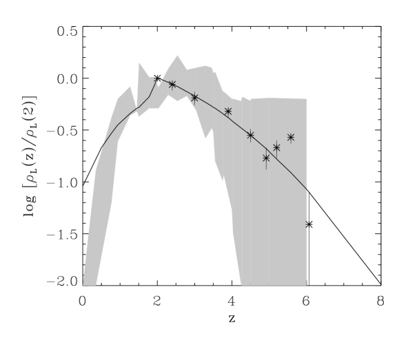
Figure 6: Integrated quasar light density vs. redshift compared to data in optical (Shaver et al., 1996) and X-rays (Miyaji et al., 2000), and the ionising flux estimated from the absorption spectra of high-$z$ quasars (McDonald & Miralda-Escudé, 2001). The model predictions are computed for the set of parameters shown in Table 1, column 5. Data and model predictions are normalised to $z=2$.

6.4 Results for the integrated quasar light

An alternate way of estimating the best values of the parameters is matching the quasar light density over the redshift range [0,6]. Note, however, that the model is very poorly constrained by the observations at $z>4$ owing to the large fraction of the quasar population that is likely to be dust-enshrouded (Xia et al., 2001; Rosati et al., 2002; Norman et al., 2002). Fig. 6 compares the model predictions with available data (the gray-shaded region). The lower limit of the observations arises from the optical data by Shaver et al. (1996), while its upper limit is deduced from X-ray measurements (e.g. Miyaji et al. 2000). We also include the data points coming from an estimate of the photoionisation rate based on the observed absorption spectra in high-$z$ quasars (Fig. 3 of McDonald & Miralda-Escudé 2001). In fact, the data used to adjust our model are the latter (normalised at $z=2$) since they are better adapted to our $\chi^{2}$ fitting procedure. Caution must be paid, however, to the fact that the total ionizing flux is believed to be dominated, at $z>4$, by that of the blue stellar population.

The predicted behaviour of the quasar light density is compatible with the observed one for intermediate and high redhifts, while there is, once again, less evolution than observed at $z<1$. Interestingly enough, the best values of the parameters obtained from the fit to the estimated ionizing background, given in column 5 of Table 1, are in general close to and, in any case, compatible with those obtained from the 2QZ sample at $z>1$. The only exceptions are $\tau_{\rm acc}$ and $M_{\rm min}$. The former takes, not surprisingly, an intermediate value between those quoted in columns 3 and 4. On the other hand, the slightly smaller value of the latter is even more consistent than the previous ones with the lower boundary of the observed mass range of current MBH masses, $10^{6}<M_{\rm BH}/M_{\odot}<10^{10}$, which corresponds to $10^{9.6}<M_{\rm H}<10^{13.6}$ at the limit $t\rightarrow\infty$ where $M_{\rm BH}\rightarrow\epsilon_{\rm G}M_{\rm G}\simeq\epsilon_{\rm G}f_{\rm b}M_{\rm H}$. This overall good agreement might indicate that quasars are the major responsible of the ionizing background at $z<4$ where the fit is very good or, alternatively, that the ratio of the contributions to this background of quasars and young stars remains approximately constant in that redshift interval.

7 DISCUSSION

We have developed a fully consistent analytical model of QLF from reasonable physical assumptions and used available data on the QLFs at various redshifts to fix the values of the free parameters. The predicted QLF agrees with the available observations at redshifts higher than $\sim 1$.

The fact that, the more accurate halo MM rate used in our model behaves essentially as the product of two PS mass functions instead of just a single one as often adopted explains the more marked positive evolution shown by the inferred QLF. Yet, the evolution so predicted is not strong enough to match the observations. The QLF calculated from the adopted MM rate but assuming a MBH mass proportional to the halo mass and the associated quasar radiating close to the Eddington regime fails to reproduce the observed data. A successful approach requires also modelling the typical evolution on cosmological timescales of MBHs and the typical lightcurve of AGN. In the present study, such a theoretical lightcurve rests on the assumptions of a phenomenological bell-shaped accretion rate and a physically grounded self-regulated radiation, while the modelling of the MBH growth is based on reasonable assumptions emanating from the expected connection between halo MMs and the reactivation of AGN.

Table 1: Best-fitting parameters, column 1, corresponding to four data sets. In columns 2 and 3, the observed QLFs drawn from the 2QZ survey in the two redshift intervals quoted. In column 4, the high-$z$ QLFs drawn essentially from the SDSS survey (Fan et al., 2001) and, in column 5, the integrated quasar light estimated from the absorption spectra of high-$z$ QSOs (McDonald & Miralda-Escudé, 2001). $z_{\rm c}$ is the redshift at which the accretion regime changes from Edington to supply-limited. $k$ is the fractional mass increase of the MBH in the Edington-limited regime. $\epsilon_{\rm G}$ is the mass ratio between the MBH and the host galaxy and $\epsilon_{\rm g}$ the ratio between the mass accreted by the MBH in a MM event and the total gas mass available, both in the supply-limited accretion regime. $\tau_{\rm acc}$ is the typical timescale of accretion onto the MBH (essentially the quasar duty cycle). $M_{\rm min}$ and $M_{\rm max}$ are the lower and upper masses of haloes likely to harbour quasars. Finally, $\nu$ is the fraction of MMs giving rise to the reactivation of one observed quasar (in the case of the integrated quasar light there is no value for $\nu$ since both the predictions and observations are normalised at $z=2$). Errors correspond to $1\sigma$ intervals, calculated in the standard way for a multiparametric fit by $\chi^{2}$ minimization. The lack of errors in the second column is due to the poor fit obtained in this case, which makes such an estimation meaningless.

	2QZ	2QZ	high-$z$	$\rho_{L}$
	$0.3<z<2.3$	$1.27<z<2.3$	$3<z<4.7$	$0<z<6$
$z_{\rm c}$	$~{}~{}~{}~{}~{}1.92$	$~{}~{}2.01^{+0.02}_{-0.02}$	$~{}4.6^{+\infty}_{-4.6}$	$~{}1.97^{+0.04}_{-0.05}$
$\epsilon_{\rm G}~{}(\times 10^{-3})$	$~{}~{}~{}~{}~{}7.91$	$~{}~{}2.45^{+0.02}_{-0.05}$	$~{}6.6^{+6.7}_{-2.6}$	$~{}2.3^{+\infty}_{-2.3}$
$\epsilon_{\rm g}~{}(\times 10^{-2})$	$~{}~{}~{}~{}~{}5.08$	$~{}~{}1.54^{+0.18}_{-0.18}$	$~{}11.0^{+\infty}_{-10.5}$	$8.5^{+\infty}_{-8.5}$
$\tau_{\rm acc}$ (Gyr)	$~{}~{}~{}~{}~{}0.05$	$~{}~{}0.18^{+0.01}_{-0.02}$	$~{}0.001^{+0.005}_{-0.001}$	$~{}0.02^{+0.06}_{-0.02}$
$k$	$~{}~{}~{}~{}~{}9.21$	$~{}~{}2.36^{+0.10}_{-0.09}$	$~{}1.0^{+4.1}_{-0.5}$	$~{}2.01^{+2.20}_{-0.17}$
$\log M_{\rm min}$ (M⊙)	$~{}~{}~{}~{}~{}10.72$	$~{}~{}12.47^{+0.01}_{-0.01}$	$~{}11.4^{+0.2}_{-\infty}$	$~{}10.0^{+0.7}_{-1.2}$
$\log M_{\rm max}$ (M⊙)	$~{}~{}~{}~{}~{}12.88$	$~{}~{}13.72^{+0.09}_{-0.04}$	$~{}14.6^{+\infty}_{-2.0}$	$~{}13.50^{+\infty}_{-0.6}$
$\nu$	$~{}~{}~{}~{}~{}0.02$	$~{}~{}0.11^{+0.01}_{-0.01}$	$~{}0.05^{+0.07}_{-0.03}$	–

The different samples of quasars studied with redshifts ranging from 1.27 to 6, lead to values of the parameters that do not differ significantly. The only relevant exception is $\tau_{\rm acc}$, the typical timescale of accretion onto the MBH, which shows a clear trend to diminish with increasing $z$ as actually expected. It is worth emphasizing that the values found for all the parameters are very reasonable. In particular, those of $\tau_{\rm acc}$, ranging from $10^{6}$ to $2\times 10^{8}$ yr according to $z$, are consistent with the most recent estimates (Yu & Tremaine 2002; Schirber & Bullock 2003). The ratio $\epsilon_{\rm G}\equiv M_{\rm BH}/M_{\rm G}$ is found to be $\simeq 2.5\times 10^{-3}$, in agreement with observations (Ferrarese & Merritt, 2000; Gebhardt et al., 2000). The fraction $\epsilon_{\rm g}$ of hot gas that ends up in the central MBH after a MM in the supply-limited accretion regime is of a few percent. The value $\sim 2$ of the parameter $k$ determining the accretion rate in the Eddington-limited regime is just what one would expect from equation (20) for a quasar of luminosity $L_{8}$, representative of a MBH of $10^{8}$ M_⊙, and a typical accretion rate of $\dot{M}_{8}$ during a duty cycle of $10^{8}$ yr. On the other hand, according to Cavaliere & Vittorini (2000), the transition between the Eddington-limited and the supply-limited accretion regimes is expected to occur at the typical formation of groups, at $z$ equal to 2.5$-$3.0, where MMs of haloes of the galactic scale become rarer and the accretion onto MBHs progressively declines. In our model, such a transition takes place when the gas fraction in baryons becomes so low that the product $\epsilon_{\rm g}M_{\rm g}$ falls below $kM_{\rm BH}$, thus becoming the limiting factor. This occurs at the epoch where $M_{\rm G}/M_{\rm g}\simeq\epsilon_{\rm g}/(k\epsilon_{\rm G})$, with the latter ratio taking a value of order unity, which is satisfied at $z_{\rm c}\sim 2$ not far from the redshifts preferred by Cavaliere & Vittorini (2000). The hosting halo masses range from $\sim 10^{11}$ M_⊙ to $\sim 10^{14}$ M_⊙, implying that quasars would be found within central galaxies of haloes from the galactic scale to the scale of galaxy groups, the structures that are currently believed to be the harbouring environments of the brightest quasars (Jäger et al. 2001). Finally, the inferred fraction of observed quasars per halo MM is found to be $\nu\simeq$ 5–10%, again pretty close to the expectations.

All these results, i.e. the good behaviour of the predicted QLFs at $z>1$ and the reasonable best-fitting values of the parameters, give strong support to the proposed connection between halo MMs and AGN lightning through the triggered simultaneous feeding of the spheroid of the main galaxy and its central MBH. The fact that our model does not match the observed evolution of QLFs at $z<1$ is also not unexpected in this scheme because of the failure for late times of that central hypothesis. The two complementary mechanisms connecting halo MMs and the reactivation of AGN imply the parallel growth of the host galaxy (by cooling flows and the merger of the main galaxies of the progenitor haloes). Consequently, they can be expected to operate as far as haloes are typically of the galactic scale, when galaxies are growing. When haloes reach the scale of galaxy groups, galaxies within them no longer grow in size, but just in number. Therefore, none of the above mentioned processes may then be effective. At such late epochs, there may still be radial flows of gas into MBHs lying at the centre of galaxies, but they should be triggered by other mechanisms —such as internal instabilities of galaxies or tidal interactions among galaxies within groups and clusters— uncorrelated with halo MMs.

These results also indicate the necessity of dealing more accurately with the physics of baryons, that is, with the processes governing the evolution of the hot gas trapped in haloes, as well as with the growth of galaxies and their interactions. In other words, a QLF model spanning from high to small redshifts should necessarily be coupled to a detailed model of galaxy formation and evolution as in the recent work by Menci et al. (2003). There are other simplifications in our model that might be also improved in future works, although they do not seem to play a crucial role on our main conclusions. There is, for instance, no consideration of the detailed physics at the vicinity of the MBH and our radiation model does not account for relativistic effects. Detailed study of the physics around the MBH could provide, for example, a natural explanation to the decrease of the number of bright quasars (Nitta 1999). Likewise, the use of an isotropic model to describe highly anisotropic radiation fields around quasars is likely to introduce different kinds of biases. The first one, due to the requirement that the line-of-sight lies in the emission cone, is of purely statistical nature and should be reasonably accounted for by the normalisation of the MM rate. A second source of bias arises from the relation between the bolometric luminosity and the MBH mass, through the Eddington efficiency, which assumes isotropy of the emission. This approximation, which cannot be corrected by a shift of the luminosity function along the magnitude axis, results in erroneous masses associated with the observed luminosities and, therefore, in erroneous merger rates. Finally, one must not forget that the comparison with observational data usually takes into account only statistical errors (very small in such large samples as the 2QZ). Systematic effects, however, like the variations of the ability of redshift determination depending on the emission lines present inside the observable wavelenght range, are likely to have a major contribution (Croom et al. 2001a).

ACKNOWLEDGMENTS

We would like to thank the people of the Toulouse Extragalactic Team as well as Hugo Capelato, Gary Mamon, Joseph Tapia and many others for help and stimulating discussions, and Brian Boyle for kindly providing us with the latest QLF of the 2QZ survey. G.M. acknowledges funding from Égide and hospitality from IAG-USP and INPE, while E.S.S. acknowledges funding from the Observatoire Midi-Pyrénées and the hospitality of its staff.

Appendix A KINETIC APPROACH FOR THE HALO MM RATE

Figure 7: Logarithm of the halo formation rate vs. redshift in the Einstein-de Sitter cosmology with an $n=0$ power-law spectrum. Two sets of curves have been inferred from the MPS model and the kinetic theory (the latter with $K=1$ in equation [27]), for hosting halo masses $M_{\rm H}=10^{12}$ M_⊙ (solid lines), $M_{\rm H}=10^{13}$ M_⊙, (dotted lines) and $10^{14}$ M_⊙ (dashed lines). On the top, logarithm of the corresponding ratio, which is constant and equal to $1550$ within 2% out to $z=20$ for $M_{\rm H}=10^{12}$ M_⊙ and within 12% out to $z=3$ for $M_{\rm H}=10^{14}$ M_⊙.

In the simplest case of an $n=0$, power-law power spectrum of density fluctuations (where there is no correlation among haloes), the merger rate is simply given, in the kinetic theory, by the usual expression

$$R(M_{\rm H},t)\,{\rm d}M_{\rm H}=\qquad\qquad\qquad\qquad\qquad\qquad\qquad\qquad$$

$$\int_{\rm P}f(M_{\rm H},t)\,{\rm d}M_{\rm H}\,f(M_{\rm PH},t)\,{\rm d}M_{\rm P}\,\langle v\,S(v)\rangle_{\rm P}\,(1+z)^{3}\,,$$ (26)

with $M_{\rm P}$ and $M_{\rm PH}\equiv M_{\rm H}-M_{\rm P}$ the masses of the primary and secondary progenitor haloes, respectively, $\langle v\,S(v)\rangle_{\rm P}$ the product of the relative velocity between the two progenitor haloes and their cross section for merger averaged over those velocities, and $(1+z)^{3}$ the factor that brings the latter product, expressed in natural units, to comoving units as the quantities entering in this expression. A reasonable approximation to adopt is

$$\langle v\,S(v)\rangle_{\rm P}=K\,\pi r_{\rm P}^{2}\,\sigma_{\rm P}\,,$$ (27)

with $r_{\rm P}$ and $\sigma_{\rm P}$ the gravitational radius and internal 3-D velocity dispersion, respectively, of the primary progenitor, which can be estimated from their scaling relations with $M_{\rm P}$. Indeed, provided all relaxed haloes have a common density contrast $\delta$, one has within the radius $r$ that $M=\delta\,r^{3}\,\rho=\delta\,r^{3}\,\rho_{0}\,\left(1+z\right)^{3}$, with $\rho$ the mean cosmic density at redshift $z$, leading to

$$r_{\rm P}\propto M_{\rm P}^{1/3}(1+z)^{-1}\,.$$ (28)

On the other hand, from the virial relation $2T+U=0$ between the halo kinetic energy $T\propto M\sigma^{2}$ and its potential energy $U\propto GM^{2}/r\propto GM^{5/3}$, the velocity dispersion takes the form

$$\sigma_{\rm P}\propto M_{\rm P}^{1/3}(1+z)^{1/2}\,.$$ (29)

Finally, the two preceding proportionalities can be calibrated from the results of Wilson et al. (2001) on galaxy-galaxy lensing which give the following parameters for a halo harbouring an $L_{\ast}$ elliptical

$$M_{\ast} = 1.3\times 10^{12}\;h^{-1}\;{\rm M_{\odot}}$$

$$r_{\ast} = 100\;(50\;\;{\rm to}\;\;200)\;h^{-1}\;{\rm kpc}$$

$$\sigma_{\ast} = 255\;(240\;\;{\rm to}\;\;270)\;{\rm km~{}s^{-1}}\,.$$

This leads to

$$r_{\rm P} = r_{\ast}\left(\frac{M_{\rm P}}{M_{\ast}}\right)^{1/3}(1+z)^{-1}$$ (30)

$$\sigma_{\rm P} = \sigma_{\ast}\left(\frac{M_{\rm P}}{M_{\ast}}\right)^{1/3}(1+z)^{1/2}\,.$$ (31)

With these approximations, the ratio between the formation rates $R_{\rm form}$ inferred from the MPS model and the kinetic theory (eqs. [3] and [26], respectively) in the Einstein-de Sitter cosmology is constant and equal to unity for $K=1550$ (see Fig. 7), except for large masses relative to the typical mass for collapse where the kinetic approach is no longer valid owing to the rarity of haloes. In this simple scale-free, $n=0$ power-law cosmology the behaviour of the MM rate as the product of two PS mass functions for moderate and small $M_{\rm H}$ can be seen from equation (2) by taking into account the corresponding explicit form of $\sigma(M_{\rm H})$. Although this is not so obvious in the general case, the fact that one always finds very similar results to those plotted in Fig. 7 allows extending that conclusion to any arbitrary cosmology.

Appendix B MBH AND HALO PROPERTIES

B.1 Growth of haloes

Figure 8: Typical time interval between MMs vs. cosmic time for halo masses ranging from $10^{11}$ to $10^{15}$ M_⊙ (top to bottom).

As shown in Fig. (8), the time dependence of $\tau_{\rm MM}(M_{\rm H},t)$ for a fixed mass $M_{\rm H}$ is very close to a power-law and the mass dependence for a fixed $t$ is not far from this simple law, too. Thus,

$$\tau_{\rm MM}(M_{\rm H},t)=\tau_{*}\,\left(\frac{t}{t_{*}}\right)^{a+1}\,\left(\frac{M_{H}}{M_{*}}\right)^{-b}\,,$$ (32)

with $\tau_{*}$, $a$ and $b$ equal to 0.73, 0.71 and 0.15, respectively, $M_{*}=10^{11}$ M_⊙ and $t_{*}=1$ Gyr. By bringing this general dependence into equation (4), we are led to

$$\frac{{\rm d}M_{\rm H}}{{\rm d}t}\approx\frac{M_{*}^{b}}{\tau_{*}}\,\,\left(\frac{t_{*}}{t}\right)^{a+1}\,\left[M_{\rm H}(t)\right]^{1-b}\,,$$ (33)

which easily integrates to

$$\left[\frac{M_{*}}{M_{\rm H}(t)}\right]^{b}=\left(\frac{M_{*}}{M_{\rm c}}\right)^{b}-B\left[\left(\frac{t_{*}}{t_{\rm c}}\right)^{a}-\left(\frac{t_{*}}{t}\right)^{a}\right]\,,$$ (34)

with $B=(bt_{*})/(a\tau_{*})$. The set of functions $\{M_{\rm H}(t)\}$ is a one-parameter family, with each member specified by its value $M_{\rm c}$ at some reference time $t_{\rm c}$.

All halo masses tend to zero as cosmic time tends to zero by virtue of equation (34). On the other hand, when time tends to infinity, the second member of equation (34) tends to

$$\left(\frac{M_{*}}{M_{\infty}}\right)^{b}=\left(\frac{M_{*}}{M_{\rm c}}\right)^{b}-B\,\left(\frac{t_{*}}{t_{\rm c}}\right)^{a}\,.$$ (35)

The requirement that both members of equation (34) are positive at all redshifts imposes a condition on $M_{\rm c}$, which cannot be arbitrarily large but has to be smaller than

$$M_{\rm top}\equiv M_{*}\left[B^{-1}\left(\frac{t_{\rm c}}{t_{*}}\right)^{a}\right]^{1/b}\hskip-3.0pt\simeq 2.7\times 10^{14}\left(\frac{t_{\rm c}}{t_{*}}\right)^{4.7}\;\hskip-3.0pt{\rm M}_{\odot}\,.$$ (36)

Otherwise, any halo of mass $M_{\rm c}>M_{\rm top}$ at time $t_{\rm c}$ would reach an infinite mass at some finite time. Conversely, given a fixed mass $M_{\rm c}=M_{\rm H}$, the corresponding time of reference $t_{\rm c}$ must be larger than the value $t_{\rm top}$ satisfying

$$t_{\rm top}=t_{*}\left[B\,\left(\frac{M_{\rm H}}{M_{*}}\right)^{b}\right]^{1/a}\,.$$ (37)

B.2 Growth of Massive Black Holes

B.2.1 Eddington-limited accretion regime

According to the assumption (6), equation (5) writes

$$\frac{{\rm d}M_{\rm BH}}{{\rm d}t}\approx k\,\frac{M_{\rm BH}[M_{\rm H}(t),t]}{\tau_{\rm MM}[M_{\rm H}(t),t]}$$ (38)

and, taking into account equation (4), we get

$$\frac{{\rm d}M_{\rm BH}}{M_{\rm BH}}\approx k\,\frac{{\rm d}M_{\rm H}}{M_{\rm H}}\,.$$ (39)

This leads, through equation (33), to

$$M_{\rm BH}(t)={M_{\rm BH}}_{\rm c}\,\left[\frac{M_{\rm H}(t)}{M_{\rm c}}\right]^{k}$$ (40)

and, from equation (6), we also get the solution $\Delta M_{\rm BH}(t)$. In equation (40), ${M_{\rm BH}}_{\rm c}$ stands for ${M_{\rm BH}}(M_{\rm c},t_{\rm c})$, the boundary condition specified below.

For any pair of physically acceptable values $({M_{\rm H}}_{i},t_{i})$ (i.e. with corresponding value of $M_{\rm c}$ at $t_{\rm c}$, determined through equation [34] for $M_{\rm H}(t_{i})={M_{\rm H}}_{i}$, satisfying the constraint [36]), the value $M_{\rm BH}({M_{\rm H}}_{i},t_{i})$ is simply equal to the solution (40) for $t=t_{i}$.

B.2.2 Supply-limited accretion regime

Equations (5) and (9) and the time derivative of equation (8) lead to

$$\frac{{\rm d}M_{\rm G}}{{\rm d}t}\approx\frac{\epsilon_{\rm g}}{\epsilon_{\rm G}}\;\frac{M_{\rm g}[M_{\rm H}(t),t]}{\tau_{\rm MM}[M_{\rm H}(t),t]}\,,$$ (41)

while equation (4) and the definition of $M_{\rm b}$ leads to

$$\frac{{\rm d}M_{\rm b}}{{\rm d}t}\approx\frac{M_{\rm b}[M_{\rm H}(t)]}{\tau_{\rm MM}[M_{\rm H}(t),t]}\,.$$ (42)

By defining the baryonic fraction in hot gas, $\gamma(M_{\rm H},t)\equiv M_{\rm g}(M_{\rm H},t)/M_{\rm b}(M_{\rm H},t)$, equations (41) and (42) lead to

$$\tau_{\rm MM}[M_{\rm H}(t),t]\;\frac{{\rm d}\gamma}{{\rm d}t}+\left(1+\frac{\epsilon_{\rm g}}{\epsilon_{\rm G}}\right)\;\gamma(t)\approx 1\,,$$ (43)

with trivial peculiar solution $\gamma_{0}$ equal to $\left(1+\epsilon/\epsilon_{\rm G}\right)^{-1}$. Then, by replacing equations (32) and (34) into equation (43) and solving the differential equation, one gets

$$\gamma(t)=\gamma_{0}+(\gamma_{\rm c}-\gamma_{0})\,\left[\frac{M_{\rm c}}{M_{\rm H}(t)}\right]^{1+\frac{\epsilon_{\rm g}}{\epsilon_{\rm G}}}\,,$$ (44)

with $\gamma_{\rm c}$ the value of $\gamma$ at $t_{\rm c}$.

As in B.2.1, for any pair of physically acceptable values $({M_{\rm H}}_{i},t_{i})$, the value $\gamma({M_{\rm H}}_{i},t_{i})$ is given by the solution (44) for $t=t_{i}$. The boundary condition $\gamma_{\rm c}=\gamma(M_{\rm c},t_{\rm c})$ necessary to find this latter solution is actually unknown, as it requires to follow in detail the physics of baryons trapped in haloes of all masses since the dark ages. However, since we expect the change in accretion regimes from Eddington to supply-limited to take place when the baryonic fraction in hot gas becomes smaller than some threshold $\gamma_{\rm c}$, we can assume that the regime changes at some time $t_{\rm c}$ (or redshift $z_{\rm c}$), for which all haloes have similar values of $\gamma$ equal to that threshold, i.e., $\gamma(M_{\rm c},t_{\rm c})=\gamma_{\rm c}$.

Therefore, for any given couple of values of $z_{\rm c}$ and $\gamma_{\rm c}$ to be determined, one can infer the function $\gamma(M_{\rm H},t)$ and, from it and equations (7)–(5), all quantities of interest; first

$$M_{\rm g}(M_{\rm H},t)=\gamma(M_{\rm H},t)\,f_{\rm b}\,M_{\rm H}\qquad\quad$$ (45)

$$M_{\rm G}(M_{\rm H},t)=[1-\gamma(M_{\rm H},t)]\,f_{\rm b}\,M_{\rm H}\,,$$ (46)

and then

$$M_{\rm BH}(M_{\rm H},t)=\epsilon_{\rm G}\,M_{\rm G}(M_{\rm H},t)\quad$$ (47)

$$\Delta M_{\rm BH}(M_{\rm H},t)=\epsilon_{\rm g}\,M_{\rm g}(M_{\rm H},t)\,.$$ (48)

The values of these two latter functions at $z_{\rm c}$ fix the boundary condition for the solution in the Eddington-limited regime, given by equations (40) and (6). Let us finally note that by dividing equation (48) by equation (47) at $z_{\rm c}$, where the solutions $M_{\rm BH}(M_{\rm H},t)$ and $\Delta M_{\rm BH}(M_{\rm H},t)$ in both regimes match and, taking into account equations (45) and (46), we obtain

$$\gamma_{\rm c}=\frac{k}{k+\frac{\epsilon_{\rm g}}{\epsilon_{\rm G}}}\,.$$ (49)

Thus, instead of $z_{\rm c}$ and $\gamma_{\rm c}$, we can use $z_{\rm c}$ and $k$ (for a given value of $\epsilon_{\rm g}/\epsilon_{\rm G}$) as the boundary conditions fixing the evolving properties of MBHs.

References

- Archibald et al. (2002) Archibald E. N., Dunlop J. S., Jimenez R., Friaça A. C. S., Mc Lure R. J., Hughes D. H., 2002, MNRAS, 336, 353
- Bond et al. (1991) Bond J. R., Cole S., Efstathiou G, Kaiser N., 1991, ApJ, 379, 440
- Bower (1991) Bower R. J., 1991, MNRAS, 248, 332
- Cavaliere & Vittorini (2000) Cavaliere A., Vittorini V., 2000, ApJ, 543, 599
- Chakrabarti (2000) Chakrabarti S. K., 2000, Class. Quant. Grav., 17, 2427
- Ciotti & Ostriker (2001) Ciotti L., Ostriker J. P., 2001, ApJ, 551,131
- Croom et al. (2001a) Croom S. M., Smith R. J., Boyle B. J., Shanks T., Loaring N. S., Miller L., Lewis I. J., 2001a, MNRAS, 322, L29
- Croom et al. (2001b) Croom S. M., Smith R. J., Boyle B. J., Shanks T., Loaring N. S., Miller L., Lewis I. J., 2001b, MNRAS, 325, 438
- Efstathiou & Rees (1988) Efstathiou G., Rees M. J., 1988, MNRAS, 230, 5
- Elvis (2002) Elvis M., 2002, Type 1 AGN Unification, in ASP Conf. Ser. 258: Issues in Unification of Active Galactic Nuclei
- Elvis et al. (1994) Elvis M. Wilkes B. J., McDowell J. C., Green R. F., Bechtold J., Willner S. P., Oey M. S., Polomski E., Cutri R., 1994, ApJS, 95, 1
- Falomo et al. (2002) Falomo R., Kotilainen J. K., Treves A., 2002, ApJ, 569, 35
- Fan et al. (2001) Fan X., Strauss M. A., Schneider D. P., Gunn J. E., Lupton R. H., Becker R. H., Davis M., Newman, J. A., Richards G. T., White R. L., Anderson J. E. Jr., Annis, J., Bahcall N. A., Brunner R. J., Csabai I., Hennessy G. S., Hindsley R. B., Fukugita M., Kunszt P. Z., Ivezic Z., Knapp G. R., McKay T. A., Munn J. A., Pier J. R., Szalay A. S., York D. G., 2001, AJ, 121, 54
- Ferrarese (2002) Ferrarese L., 2002, ApJ, 578, 90
- Ferrarese & Merritt (2000) Ferrarese L., Merritt D., 2000, ApJ, 539, L9
- Gebhardt et al. (2000) Gebhardt K., Bender R., Bower G., Dressler A., Faber S. M., Filippenko A. V., Green R., Grillmair C., Ho L. C., Kormendy J., Lauer T. R., Magorrian J., Pinkney J., Richstone D., Tremaine S., 2000, ApJ, 539, L13
- Granato et al. (2001) Granato G. L., Silva L., Monaco P., Panuzzo P., Salucci P., De Zotti G., Danese L., 2001, MNRAS, 324, 757
- Haehnelt & Rees (1993) Haehnelt M. G., Rees M. J., 1993, MNRAS, 263, 168
- Haehnelt et al. (1998) Haehnelt M. G., Natarajan P. Rees M. J., 1998, MNRAS, 300, 817
- Haiman & Loeb (1998) Haiman Z.. Loeb A., 1998, ApJ, 503, 505
- Haiman & Menou (2000) Haiman Z.. Menou K., 2000, ApJ, 531, 42
- Hatziminaoglou et al. (2001) Hatziminaoglou E., Siemiginowska A. Elvis, M., 2001, ApJ
- Jäger et al. (2001) Jäger K., Fricke K. J., Heidt J., 2001, in A large Survey of Quasar Environments, Astronomische Gesellschaft Meeting Abstracts, 18, 516
- Kauffmann & Haehnelt (2000) Kauffmann G., Haehnelt M., 2000, MNRAS, 311, 576
- Kennefick et al. (1995) Kennefick J. D., Djorgovski S. G., de Carvalho R. R., 1995, AJ, 110, 2553
- Kennefick et al. (1996) Kennefick J. D., Djorgovski S. G., Meylan G., 1996, AJ, 111, 1816
- Kormendy & Richstone (1995) Kormendy J., Richstone D., 1995, ARAA, 33, 581
- Kormendy & Gebhardt (2001) Kormendy J., Gebhardt K., 2001, Supermassive Black Holes in Nuclei of Galaxies, in the 20th Texas Symposium on Relativistic Astrophysics, ed. H. Martel & J. C. Wheeler, AIP
- Lacey & Cole (1993) Lacey C., Cole S., 1993, MNRAS, 262, 627
- Martini & Weinberg (2001) Martini P., Weinberg D. H., 2001, ApJ, 547, 12
- McLure & Dunlop (2001) McLure R. J., Dunlop J. S., 2001, MNRAS, 327, 199
- Magorrian et al. (1998) Magorrian J., Tremaine S., Richstone D., Bender R., Bower G., Dressler A., Faber S. M., Gebhardt K., Green R., Grillmair C.., Kormendy J., Lauer T., 1998, AJ, 115, 2285
- Manrique et al. (2003) Manrique A., Raig A., Sanchis T., Salvador-Solé E., Solanes J. M., 2003, ApJ, submitted
- McDonald & Miralda-Escudé (2001) McDonald P., Miralda-Escudé J., 2001, ApJ, 549, L11
- Menci et al. (2003) Menci N., Cavaliere A., Fontana A., Giallongo E., Poli F., Vittorini V., 2003, ApJ, submitted (astro-ph/0303332)
- Merritt & Ferrarese (2001) Merritt D., Ferrarese L., 2001, ApJ, 547, 140
- Miyaji et al. (2000) Miyaji T., Hasinger G., Schmidt M., 2000, AA, 353, 25
- Monaco et al. (2000) Monaco P., Salucci P., Danese L., 2000, MNRAS, 311, 278
- Mortlock et al. (1999) Mortlock D. J., Webster R. L., Francis P. J., 1999, MNRAS, 309, 836
- Navarro, Frenk & White (1997) Navarro J. F., Frenk C. S., White S. D. M., 1997, ApJ, 490, 493
- Nitta (1999) Nitta S.-Y., 1999, MNRAS, 308, 995
- Norman et al. (2002) Norman C., Hasinger G., Giacconi R., Gilli R., Kewley L., Nonino M., Rosati P., Szokoly G., Tozzi P., Wang J., Zheng W., Zirm A., Bergeron J., Gilmozzi R., Grogin N., Koekemoer A., Schreier E., 2002, 571, 218
- Percival, Miller & Peacock (2000) Percival W. J., Miller, L., Peacock, J. A., 2000, MNRAS, 318, 273
- Press & Schechter (1974) Press W. H., Schechter P., 1974, ApJ, 193, 437
- (45) Raig A., González-Casado G., Salvador-Solé E., 1998, ApJ, 508, L129
- (46) Raig A., González-Casado G., Salvador-Solé E., 2001, MNRAS, 327, 939
- Rosati et al. (2002) Rosati P., Tozzi P., Giacconi R., Gilli R., Hasinger G., Kewley L., Mainieri V., Nonino M., Norman C., Szokoly G., Wang J. X., Zirm A., Bergeron J., Borgani S., Gilmozzi R., Grogin N., Koekemoer A., Schreier E., Zheng W., 2002, ApJ, 566, 667
- (48) Salvador-Solé E., Solanes J. M., Manrique A., 1998, ApJ, 499, 542
- Shaver et al. (1996) Shaver P. A., Wall J. V., Kellermann K. I., Jackson C. A., Hawkins M. R. S., 1996, Nature, 384, 439
- Schirber & Bullock (2003) Schirber M., Bullock J. S., 2003, ApJ, 584, 110
- Schmidt et al. (1995) Schmidt M., Schneider D. P., Gunn J. E., 1995, AJ, 110, 68
- Siemiginowska & Elvis (1997) Siemiginowska A., Elvis M., 1997, ApJ, 482, L9
- (53) Silk, J., Rees, M., 1998, AA, 331, L1
- Tremaine et al. (2002) Tremaine, S., Gebhardt, K., Bender, R., Bower, G., Dressler, A., Faber, S. M., Filippenko, A. V., Green, R., Grillmair, C., Ho, L. C., Kormendy, J., Lauer, T. R., Magorrian, J., Pinkney, J., Richstone, D., 2002, ApJ, 574, 740
- Volonteri, Haardt & Madau (2003) Volonteri, M., Haardt, F., Madau, P., 2003, ApJ, 582, 559
- Wandel (1999) Wandel A., 1999, ApJ, 519, L39
- Wandel (2002) Wandel A., 2002, ApJ, 565, 762
- Wilson et al. (2001) Wilson G., Kaiser N., Luppino G. A., Cowie L., 2001, ApJ, 555, 572
- Woo & Urry (2002) Woo J.-H., Urry, C.M., 2002, ApJ, 579, 530
- Wu et al. (2002) Wu, X.B., Liu, F.K., Zhang, T.Z. 2002, AA, 389, 742
- Wyithe & Loeb (2002) Wyithe J. S. B., Loeb, A., 2002, ApJ, 581, 886
- Xia et al. (2001) Xia X. Y., Boller T., Deng Z. G., Börner G., 2001, ChJAA, 1, 221
- Yu & Tremaine (2002) Yu Q., Tremaine S., 2002, ApJ, 335, 965