Large-scale curvature and entropy perturbations for multiple interacting fluids

Abstract

We present a gauge-invariant formalism to study the evolution of curvature perturbations in a Friedmann-Robertson-Walker universe filled by multiple interacting fluids. We resolve arbitrary perturbations into adiabatic and entropy components and derive their coupled evolution equations. We demonstrate that perturbations obeying a generalised adiabatic condition remain adiabatic in the large-scale limit, even when one includes energy transfer between fluids. As a specific application we study the recently proposed curvaton model, in which the curvaton decays into radiation. We use the coupled evolution equations to show how an initial isocurvature perturbation in the curvaton gives rise to an adiabatic curvature perturbation after the curvaton decays.

I Introduction

The primordial curvature perturbation plays a central role in modern cosmology. It characterises large-scale density perturbations in our Universe from which smaller scale structures form via gravitational instability. Therefore much effort has been devoted to understanding the evolution of the curvature perturbation on large-scales in a general cosmology. A gauge-invariant formalism for cosmological metric perturbations was developed by Bardeen Bardeen and the curvature perturbation (on uniform density hypersurfaces) $\zeta$ was introduced by Bardeen et al. BST ; Bardeen88 shortly afterwards as a convenient gauge-invariant variable which remains constant for purely adiabatic perturbations on large scales. On large scales in an expanding universe it is essentially equivalent to the comoving density perturbation Lukash ; Lyth1985 ; MFB .

The constancy of the curvature perturbation $\zeta$ in the case of a single perfect fluid follows directly from the local conservation of the energy-momentum tensor, in a suitably defined large-scale limit WMLL . But $\zeta$ can change on arbitrarily large scales due to a non-adiabatic pressure perturbation Mollerach ; MFB ; GBW ; WMLL . Thus in a multi-fluid system it is in general necessary to follow the coupled evolution of curvature and entropy (or isocurvature) perturbations in order to determine the late-time curvature perturbation.

There has been increasing interest in multi-field inflationary models and the spectrum of curvature Polarski1 ; Starobinsky ; SS ; GBW ; MS and isocurvature Polarski2 ; LM perturbations that may be produced and their correlations Langlois ; chris . In particular it has recently been suggested that the large-scale curvature perturbation $\zeta$ may be generated by initial isocurvature perturbations in a “curvaton” field which subsequently decays into radiation Enqvist ; curvaton ; MT ; LUW .

Kodama and Sasaki KS developed a general formalism to describe the evolution of cosmological perturbations with multiple fluids (with corrections given in hama ). This formalism has subsequently been used by a number of authors KSrad1 ; KSrad2 ; hama ; Hwang:fluids ; Mar (see also bruni ; nambu ; dehnen ). In particular Kodama and Sasaki applied their formalism to a matter-radiation fluid in KSrad1 ; KSrad2 , where energy transfer can be neglected. One can argue on general grounds WMLL that the entropy perturbations evolve independently of the curvature perturbation on large scales, but that the evolution of the large-scale curvature is sourced by entropy perturbations. Nonetheless there has been no detailed study of the evolution in general of curvature and entropy perturbations including energy transfer. By contrast a formalism to study the coupled evolution equations for curvature and entropy perturbations in models with multiple interacting scalar fields has recently been developed by Gordon et al. chris and applied in a variety of scenarios BMR ; NR ; Finelli ; Ashcroft (see also Hwang:fields ; nibbelink ).

In this paper we introduce a gauge-invariant formalism to follow the coupled evolution of curvature and entropy perturbations in multi-fluid cosmologies when energy transfer between fluids is included. As an example we study the evolution of curvature and entropy perturbations in a curvaton scenario where the decay of the curvaton field represents the transfer of energy from the curvaton to radiation. We compare the results of numerical solutions of the coupled equations with analytic estimates based on the sudden decay approximation, where the curvaton and radiation are assumed to be non-interacting up until a given decay time.

II Governing equations

In this section we give the governing equations for the general case of an arbitrary number of interacting fluids in general relativity. We will consider linear perturbations about a spatially-flat FRW background model, as defined by the line element

$$ds^{2}=-(1+2\phi)dt^{2}+2aB_{,i}dtdx^{i}+a^{2}\left[(1-2\psi)\delta_{ij}+2E_{,ij}\right]dx^{i}dx^{j}\,,$$ (1)

where we use the notation of Ref.MFB for the gauge-dependent curvature perturbation, $\psi$, the lapse function, $\phi$, and scalar shear, $\chi\equiv a^{2}\dot{E}-aB$.

Each fluid has an energy-momentum tensor $T^{\mu\nu}_{(\alpha)}$. The total energy momentum tensor $T^{\mu\nu}=\sum_{\alpha}T^{\mu\nu}_{(\alpha)}$, is covariantly conserved, but we allow for energy transfer between the fluids,

$$\nabla_{\mu}T^{\mu\nu}_{(\alpha)}=Q^{\nu}_{(\alpha)}\,,$$ (2)

where $Q^{\nu}_{(\alpha)}$ is the energy-momentum transfer to the $\alpha$-fluid, which is subject to the constraint

$$\sum_{\alpha}Q^{\nu}_{(\alpha)}=0\,.$$ (3)

The equations hold for any type of fluid, the only requirement being the local conservation of the total energy-momentum tensor, $\nabla_{\mu}T^{\mu\nu}=0$.

II.1 Background equations

The evolution of the background FRW universe is governed by the Friedmann constraint

$$H^{2} = \frac{8\pi G}{3}\rho\,,$$ (4)

and the continuity equation

$$\dot{\rho}=-3H\left(\rho+P\right)\,,$$ (5)

where the dot denotes a derivative with respect to coordinate time $t$, $H\equiv\dot{a}/a$ is the Hubble parameter, and $\rho$ and $P$ are the total energy density and the total pressure

$$\sum_{\alpha}\rho_{\alpha}=\rho\,,\qquad\sum_{\alpha}P_{\alpha}=P\,.$$ (6)

The continuity equation for each individual fluid in the background is thus KS

$$\dot{\rho}_{\alpha}=-3H\left(\rho_{\alpha}+P_{\alpha}\right)+Q_{\alpha}\,,$$ (7)

where the energy transfer to the $\alpha$ fluid is given by the time component of the energy-momentum transfer vector $Q^{0}_{(\alpha)}=Q_{\alpha}$ in the background. Equation (3) implies that the background energy transfer obeys the constraint

$$\sum_{\alpha}Q_{\alpha}=0\,.$$ (8)

II.2 Perturbed equations

Perturbing the constraint equation (4) yields the first-order equation KS ; MFB ; thesis

$$3H\left(\dot{\psi}+H\phi\right)-\frac{\nabla^{2}}{a^{2}}\left(\psi+H\chi\right)=-4\pi G\delta\rho\,,$$ (9)

where the comoving spatial Laplacian is denoted by $\nabla^{2}\equiv\partial^{2}/\partial x^{i2}$, and the momentum constraint equation (identically zero in the FRW background) is given by KS ; MFB ; thesis

$$\dot{\psi}+H\phi=-4\pi G{\delta q}\,,$$ (10)

where $\delta\rho$ is the density perturbation and $\delta q$ the scalar 3-momentum potential.

Perturbing the continuity equation (5) yields an evolution equation for the total density perturbation KS ; thesis

$$\dot{\delta\rho}+3H(\delta\rho+\delta P)-\left(\rho+P\right)3\dot{\psi}+\frac{\nabla^{2}}{a^{2}}\left[{\delta q}+(\rho+P)\chi\right]=0\,,$$ (11)

while total momentum conservation is given by KS ; thesis

$$\dot{\delta q}+3H{\delta q}+(\rho+P)\phi+\delta P+\frac{2}{3}\frac{\nabla^{2}}{a^{2}}\Pi=0\,,$$ (12)

where $\Pi$ is the total anisotropic stress.

The perturbed energy transfer vector, Eq. (2), including terms up to first order, is written as KS

$$Q_{(\alpha)0} = -Q_{\alpha}(1+\phi)-\delta Q_{\alpha}\,,$$ (13)

$$Q_{(\alpha)i} = \left(f_{\alpha}+\frac{Q_{\alpha}}{\rho+P}{\delta q}\right)_{,i}\,,$$ (14)

and Eq. (3) implies that the perturbed energy and momentum transfer obey the constraints

$$\sum_{\alpha}\delta Q_{\alpha}=0\,,\quad\sum_{\alpha}f_{\alpha}=0\,.$$ (15)

The perturbed energy conservation equation for a particular fluid, including energy transfer, is then given by

$$\dot{\delta\rho}_{\alpha}+3H(\delta\rho_{\alpha}+\delta P_{\alpha})-\left(\rho_{\alpha}+P_{\alpha}\right)3\dot{\psi}+\frac{\nabla^{2}}{a^{2}}\left[{\delta q_{\alpha}}+(\rho_{\alpha}+P_{\alpha})\chi\right]=Q_{\alpha}\phi+\delta Q_{\alpha}\,,$$ (16)

while the momentum conservation equation is

$$\dot{\delta q_{\alpha}}+3H{\delta q_{\alpha}}+(\rho_{\alpha}+P_{\alpha})\phi+\delta P_{\alpha}+\frac{2}{3}\frac{\nabla^{2}}{a^{2}}\Pi_{\alpha}=Q_{\alpha}\frac{{\delta q}}{\rho+P}+f_{\alpha}\,,$$ (17)

where the density, pressure, momentum and anisotropic stress perturbations of the individual fluids are related to the total density, pressure, momentum and anisotropic stress perturbations by

$$\sum_{\alpha}\delta\rho_{\alpha}=\delta\rho\,,\qquad\sum_{\alpha}\delta P_{\alpha}=\delta P\,,\qquad\sum_{\alpha}{\delta q_{\alpha}}={\delta q}\,,\qquad\sum_{\alpha}\Pi_{\alpha}=\Pi\,.$$ (18)

II.3 Gauge-invariant perturbations

Both the density perturbation, $\delta\rho_{\alpha}$, and the curvature perturbation, $\psi$, are in general gauge-dependent. Specifically they depend upon the chosen time-slicing in an inhomogeneous universe. However a gauge-invariant combination can be constructed which describes the density perturbation on uniform curvature slices or, equivalently the curvature of uniform density slices.

The curvature perturbation on uniform total density hypersurfaces, $\zeta$, is given by BST ; WMLL

$$\zeta=-\psi-H\frac{\delta\rho}{\dot{\rho}}\,,$$ (19)

while the curvature perturbation on uniform $\alpha$-fluid density hypersurfaces, $\zeta_{\alpha}$, is defined asWMLL

$$\zeta_{\alpha}=-\psi-H\frac{\delta\rho_{\alpha}}{\dot{\rho}_{\alpha}}\,.$$ (20)

The total curvature perturbation (19) is thus a weighted sum of the individual perturbations

$$\zeta=\sum_{\alpha}\frac{\dot{\rho}_{\alpha}}{\dot{\rho}}\zeta_{\alpha}\,,$$ (21)

while the difference between any two curvature perturbations describes a relative entropy (or isocurvature) perturbation

$${\cal{S}}_{\alpha\beta}=3(\zeta_{\alpha}-\zeta_{\beta})=-3H\left(\frac{\delta\rho_{\alpha}}{\dot{\rho}_{\alpha}}-\frac{\delta\rho_{\beta}}{\dot{\rho}_{\beta}}\right)\,.$$ (22)

The classic example of just such a relative entropy perturbation is a perturbation in the primordial baryon-photon ratio (with negligible energy transfer between the two fluids)

$${\cal{S}}_{B\gamma}=3(\zeta_{B}-\zeta_{\gamma})=\frac{\delta\rho_{B}}{\rho_{B}}-\frac{3}{4}\frac{\delta\rho_{\gamma}}{\rho_{\gamma}}\,.$$ (23)

This is also described as an initial isocurvature baryon density perturbation as ${\cal{S}}_{B\gamma}\to\delta\rho_{B}/\rho_{B}$ in the limit $\rho_{B}/\rho_{\gamma}\to 0$.

From the definitions of the total curvature perturbation (21) and the entropy perturbation (22), we get

$$\zeta_{\alpha}=\zeta+\frac{1}{3}\sum_{\beta}\frac{\dot{\rho}_{\beta}}{\dot{\rho}}{\cal{S}}_{\alpha\beta}\,.$$ (24)

II.4 Long-wavelength limit

To describe the evolution of long-wavelength perturbations we will work in the ‘separate universes’ picture WMLL where, smoothing over sufficiently large scales, the universe looks locally like an unperturbed (FRW) cosmology. Specifically we assume that we can neglect the divergence of the momenta in the zero-shear gauge, $\nabla^{2}(\delta q_{\alpha}+(\rho_{\alpha}+P_{\alpha})\chi)$, in Eq. (16).

In this long-wavelength limit, the perturbed continuity equation (11) becomes

$$\dot{\delta\rho}+3H(\delta\rho+\delta P)=3\left(\rho+P\right)\dot{\psi}\,.$$ (25)

Re-writing this equation in terms of the total curvature perturbation, $\zeta$ in Eq. (19), gives GBW ; WMLL

$$\dot{\zeta}=-\frac{H}{\rho+P}\delta P_{\rm nad}\,,$$ (26)

where the non-adiabatic pressure perturbation is $\delta P_{\rm nad}\equiv\delta P-c_{\rm{s}}^{2}\delta\rho$ and the adiabatic sound speed is $c_{\rm{s}}^{2}=\dot{P}/\dot{\rho}$. Thus the total curvature perturbation is constant on large scales for purely adiabatic perturbations.

In the presence of more than one fluid, the total non-adiabatic pressure perturbation, $\delta P_{\rm nad}$, may be split into two parts,

$$\delta P_{\rm nad}\equiv\delta P_{\rm intr}+\delta P_{\rm rel}\,.$$ (27)

The first part is due to the intrinsic entropy perturbation of each fluid

$$\delta P_{\rm intr}=\sum_{\alpha}\delta P_{\rm{intr},\alpha}\,,$$ (28)

where the intrinsic non-adiabatic pressure perturbation of each fluid is given by

$$\delta P_{\rm{intr},\alpha}\equiv\delta P_{\alpha}-c^{2}_{\alpha}\delta\rho_{\alpha}\,,$$ (29)

$c^{2}_{\alpha}\equiv\dot{P}_{\alpha}/\dot{\rho}_{\alpha}$ is the adiabatic sound speed of that fluid and the total adiabatic sound speed is the weighted sum of the adiabatic sound speeds of the individual fluids,

$$c^{2}_{\rm{s}}=\sum_{\alpha}\frac{\dot{\rho}_{\alpha}}{\dot{\rho}}c^{2}_{\alpha}\,.$$ (30)

The second part of the non-adiabatic pressure perturbation (27) is due to the relative entropy perturbation between different fluids, denoted by $\cal{S}_{\alpha\beta}$ in Eq. (22),

$$\delta P_{\rm rel}\equiv\frac{1}{6H\dot{\rho}}\sum_{\alpha,\beta}\dot{\rho}_{\alpha}\dot{\rho}_{\beta}\left(c^{2}_{\alpha}-c^{2}_{\beta}\right){\cal{S}}_{\alpha\beta}\,.$$ (31)

The time-dependence of the intrinsic entropy perturbation, $\delta P_{{\rm intr},\alpha}$, of each fluid must be specified according to the detailed modelling of that fluid. For instance, if the fluid has a definite equation of state $P_{\alpha}=P_{\alpha}(\rho_{\alpha})$ then the intrinsic non-adiabatic pressure perturbation vanishes.

The evolution of the relative entropy perturbation, $\cal{S}_{\alpha\beta}$, follows from the time dependence of the individual curvature perturbations $\zeta_{\alpha}$ and $\zeta_{\beta}$. Equation (16) for the evolution of the gauge-dependent density perturbations in the long-wavelength limit reduces to

$$\dot{\delta\rho}_{\alpha}+3H(\delta\rho_{\alpha}+\delta P_{\alpha})=3\left(\rho_{\alpha}+P_{\alpha}\right)\dot{\psi}+Q_{\alpha}\phi+\delta Q_{\alpha}\,.$$ (32)

Re-writing this in terms of the gauge-invariant curvature perturbation $\zeta_{\alpha}$ defined in (20) gives an evolution equation for the curvature perturbation on uniform $\alpha$-fluid density hypersurfaces,

$$\dot{\zeta}_{\alpha} = \frac{3H^{2}}{\dot{\rho}_{\alpha}}\left[\delta P_{\alpha}-c^{2}_{\alpha}\delta\rho_{\alpha}\right]-{HQ_{\alpha}\over\dot{\rho}_{\alpha}}\left[{\delta Q_{\alpha}\over Q_{\alpha}}+\left({\dot{\rho}\over 2\rho}-{\dot{Q}_{\alpha}\over Q_{\alpha}}\right){\delta\rho_{\alpha}\over\dot{\rho}_{\alpha}}+H^{-1}\dot{\psi}+\phi\right]$$ (33)

$$= \frac{3H^{2}\delta P_{\rm{intr},\alpha}}{\dot{\rho}_{\alpha}}-{H\delta Q_{\rm{nad},\alpha}\over\dot{\rho}_{\alpha}}\,.$$

For non-interacting, perfect fluids ($Q_{\alpha}=0$ and $\delta P_{{\rm intr},\alpha}=0$) we have $\dot{\zeta}_{\alpha}=0$ and the individual curvature perturbations for each fluid remain constant in the long-wavelength limit WMLL . But in general, the curvature perturbation $\zeta_{\alpha}$ may change with time either due to the intrinsic non-adiabatic pressure perturbation, $\delta P_{{\rm intr},\alpha}$ in Eq. (29) or due to what we will call the ‘non-adiabatic’ energy transfer, $\delta Q_{\rm{nad},\alpha}$.

Analogously to the total non-adiabatic pressure perturbation (27), we will split the non-adiabatic energy transfer into two parts,

$$\delta Q_{{\rm nad},\alpha}\equiv\delta Q_{{\rm intr},\alpha}+\delta Q_{{\rm rel},\alpha}\,.$$ (34)

The first part is the instrinsic non-adiabatic energy transfer perturbations, defined as

$$\delta Q_{{\rm intr},\alpha}\equiv\delta Q_{\alpha}-{\dot{Q}_{\alpha}\over\dot{\rho}_{\alpha}}\delta\rho_{\alpha}\,.$$ (35)

This is automatically zero if the local energy transfer $Q_{\alpha}$ is a function of the local density $\rho_{\alpha}$ so that $\delta Q_{\alpha}=\dot{Q}_{\alpha}\delta\rho_{\alpha}/\dot{\rho}_{\alpha}$, just as the intrinsic non-adiabatic pressure perturbation (29) vanishes when $\delta P_{\alpha}=\dot{P}_{\alpha}\delta\rho_{\alpha}/\dot{\rho}_{\alpha}$. The second part is the relative non-adiabatic energy transfer

$$\delta Q_{{\rm rel},\alpha}={Q_{\alpha}\dot{\rho}\over 2\rho}\left({\delta\rho_{\alpha}\over\dot{\rho}_{\alpha}}-{\delta\rho\over\dot{\rho}}\right)=-{Q_{\alpha}\over 6H\rho}\sum_{\beta}\dot{\rho}_{\beta}{\cal{S}}_{\alpha\beta}\,,$$ (36)

where we have used the background Einstein equations (4) and the perturbed Friedmann constraint equation (9) on large scales,

$$\dot{\psi}+H\phi=-\frac{H}{2}\frac{\delta\rho}{\rho}\,,$$ (37)

in order to write $\delta Q_{{\rm rel},\alpha}$ explicitly in terms of the relative entropy perturbation, ${\cal{S}}_{\alpha\beta}$.

Note that the relative non-adiabatic pressure perturbation, defined in Eq. (31) is related to the relative non-adiabatic energy transfer perturbation defined in Eq. (36) as

$$\delta P_{\rm{rel}}=-2\frac{\rho}{\dot{\rho}}\sum_{\alpha}\frac{\dot{\rho}_{\alpha}c^{2}_{\alpha}}{Q_{\alpha}}\delta Q_{{\rm rel},\alpha}\,.$$ (38)

The non-adiabatic pressure perturbations, $\delta P_{\rm{intr},\alpha}$ and $\delta P_{\rm rel}$, and the non-adiabatic energy transfers, $\delta Q_{\rm{intr},\alpha}$ and $\delta Q_{\rm{rel},\alpha}$, are all automatically gauge-invariant. The intrinsic entropy perturbations, $\delta P_{\rm{intr},\alpha}$ and $\delta Q_{\rm{intr},\alpha}$, are both zero if the pressure and local energy transfer are determined by the local energy density. But even if the intrinsic entropy perturbations vanish, there may be a non-adiabatic energy transfer due to the relative entropy perturbation, $\zeta-\zeta_{\alpha}$. We interpret this as due to a gravitational redshift (time-dilation) which perturbs the rate of energy transfer with respect to coordinate time if the uniform $\alpha$-density hypersurface does not coincide with the uniform total density hypersurface, $\zeta_{\alpha}\neq\zeta$.

By taking the difference between the evolution equations (33) for two fluids we obtain an evolution equation for the relative entropy perturbation on large scales

$$\dot{\cal{S}}_{\alpha\beta}=3H\left(\frac{3H\delta P_{\rm{intr},\alpha}-\delta Q_{\rm{intr},\alpha}}{\dot{\rho}_{\alpha}}-\frac{3H\delta P_{\rm{intr},\beta}-\delta Q_{\rm{intr},\beta}}{\dot{\rho}_{\beta}}\right)+\sum_{\gamma}{\dot{\rho}_{\gamma}\over 2\rho}\left({Q_{\alpha}\over\dot{\rho}_{\alpha}}{\cal{S}}_{\alpha\gamma}-{Q_{\beta}\over\dot{\rho}_{\beta}}{\cal{S}}_{\beta\gamma}\right)\,.$$ (39)

Thus we see that any relative entropy perturbation ${\cal{S}}_{\alpha\beta}$ is sourced on large scales only by intrinsic entropy perturbations in the $\alpha$ and $\beta$ fluid, or by other relative entropy perturbations. There is no source term coming from the overall curvature perturbation and so adiabatic perturbations (with no intrinsic or relative entropy perturbation) remain adiabatic on large-scales even when one considers interacting fluids.

III Curvaton decay

Having established a general formalism in which to study the evolution of large-scale curvature and entropy perturbations including entropy transfer between multiple fluids, we now study the specific case of a non-relativistic matter decaying into radiation. In particular this can be used to describe the decay of a massive curvaton field into radiation Enqvist ; curvaton ; MT ; LUW .

The curvaton scenario has recently been proposed  Enqvist ; curvaton ; MT ; LUW as a mechanism by which a large-scale curvature perturbation can be produced from an initially isocurvature perturbation. If the curvaton is a light scalar field (with mass less than the Hubble rate) the field may acquire an almost scale-invariant spectrum of perturbations, $\zeta_{\sigma}$. In the curvaton scenario radiation, $\rho_{\gamma}$, is supposed to dominate the initial energy density after inflation and this is assumed to be unperturbed, $\zeta_{\gamma}=0$. Thus the curvaton perturbation is initially an isocurvature density perturbation ($\zeta\simeq 0$ and ${\cal{S}}_{\sigma\gamma}=3\zeta_{\sigma}$) and remains an isocurvature perturbation while the relative density of the curvaton remains negligible. However, once the Hubble rate drops below the mass of the curvaton, the field begins to oscillate. Averaged over several oscillations the effective equation of state is $\langle P_{\sigma}/\rho_{\sigma}\rangle=0$, i.e., the coherent oscillations of the field are equivalent to a fluid of non-relativistic particles Turner . As the energy density of non-relativistic particles grows relative to the energy density of radiation, what was once an isocurvature perturbation becomes a perturbation in the total curvature, Eq. (21).

Assuming the curvaton is unstable and decays into light particles (“radiation”) with a decay rate $\Gamma$, this represents an energy transfer from the pressureless curvaton fluid to the radiation fluid. The precise amplitude of the resulting curvature perturbation, relative to the initial curvaton perturbation, depends upon both the initial density and the decay rate of the curvaton. We present the equations for the evolution of the curvature and relative entropy perturbations and solve them numerically, comparing with an analytic approximation assuming an instantaneous decay.

III.1 Background solution

The energy transfer from the massive curvaton to light radiation is described by

$$Q_{\sigma} = -\Gamma\rho_{\sigma}\,,$$ (40)

$$Q_{\gamma} = \Gamma\rho_{\sigma}\,,$$ (41)

where $\Gamma$ is the decay rate of the curvaton into radiation, which we take to be a constant. The energy conservation equations are therefore

$$\dot{\rho}_{\sigma} = -\rho_{\sigma}\left(3H+\Gamma\right)\,,$$ (42)

$$\dot{\rho}_{\gamma} = -4H\rho_{\gamma}+\Gamma\rho_{\sigma}\,,$$ (43)

$$\dot{\rho} = -H\left(3\rho_{\sigma}+4\rho_{\gamma}\right)\,,$$ (44)

where the Hubble expansion is given by

$$H^{2}={8\pi G\over 3}\left(\rho_{\sigma}+\rho_{\gamma}\right)\,.$$ (45)

In order to solve the system of equations above numerically, it is convenient to work in terms of the dimensionless density parameters

$$\Omega_{\sigma}\equiv\frac{\rho_{\sigma}}{\rho}\,,\quad\Omega_{\gamma}\equiv\frac{\rho_{\gamma}}{\rho}\,,$$ (46)

and the dimensionless “reduced” decay rate

$$\quad g\equiv\frac{\Gamma}{\Gamma+H}\,,$$ (47)

which varies monotonically from $0$ to $1$ in an expanding universe.

The background equations (42-45) can then be written as an autonomous system

$$\Omega_{\sigma}^{\prime} = \Omega_{\sigma}\left(\Omega_{\gamma}-{g\over 1-g}\right)\,,$$ (48)

$$\Omega_{\gamma}^{\prime} = \Omega_{\sigma}\left({g\over 1-g}-\Omega_{\gamma}\right)\,,$$ (49)

$$g^{\prime} = {1\over 2}(4-\Omega_{\sigma})(1-g)g\,,$$ (50)

where ^′ denotes differentiation with respect to the number of e-foldings $N\equiv\ln a$. The density parameters are subject to the Friedmann constraint (45) which requires

$$\Omega_{\sigma}+\Omega_{\gamma}=1\,.$$ (51)

There are only two independent dynamical equations and the generic solutions follow trajectories in a compact two-dimensional phase-plane ($0\leq g\leq 1$, $0\leq\Omega_{\sigma}\leq 1$), illustrated in Figure 1.

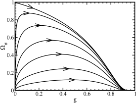
Figure 1: Phase-plane showing trajectories for the background solutions in the curvaton model in Eqs.(48–51).

The dynamical system (48–51) admits three fixed points

(A)

$\Omega_{\gamma}=1$, $\Omega_{\sigma}=0$, $g=0$,

(B)

$\Omega_{\gamma}=0$, $\Omega_{\sigma}=1$, $g=0$,

(C)

$\Omega_{\gamma}=1$, $\Omega_{\sigma}=0$, $g=1$.

Generic solutions start at the unstable repellor $(A)$ and approach the stable attractor $(C)$ at late times. At early times ($\Omega_{\gamma}\simeq 1$, $g\ll 1$) we find $g\propto\Omega_{\sigma}^{2}\propto a^{2}$. The standard radiation dominated cosmology corresponds to evolution along the line $\Omega_{\sigma}=0$. However solutions can approach arbitrarily close the curvaton-dominated saddle point $(B)$ before the curvaton decays and $\Omega_{\sigma}\to 0$ once again.

III.2 Perturbations

Both the curvaton and radiation fluids have fixed equations of state ($\delta P_{\sigma}=0$ and $\delta P_{\gamma}=\delta\rho_{\gamma}/3$) and hence there can be no intrinsic non-adiabatic pressure perturbation ($\delta P_{{\rm intr},\sigma}=0$ and $\delta P_{{\rm intr},\gamma}=0$). However the total curvature perturbation, $\zeta$, does change on large scales in the presence of a relative entropy perturbation (22)

$${\cal{S}}_{\sigma\gamma}\equiv 3(\zeta_{\sigma}-\zeta_{\gamma})\,,$$ (52)

which leads to a non-adiabatic pressure perturbation (31). The evolution of the total curvature perturbation $\zeta$, using Eqs. (26), is

$$\dot{\zeta}={H\over 3}\frac{\dot{\rho}_{\sigma}\dot{\rho}_{\gamma}}{\dot{\rho}^{2}}{\cal{S}}_{\sigma\gamma}\,.$$ (53)

We assume that the curvaton decay rate $\Gamma$ is fixed by microphysics (i.e., $\delta\Gamma=0$) and hence the perturbed energy transfer is simply given by

$$\delta Q_{\sigma} = -\Gamma\delta\rho_{\sigma}\,,$$ (54)

$$\delta Q_{\gamma} = \Gamma\delta\rho_{\sigma}\,.$$ (55)

This energy transfer is determined solely by the local density of the curvaton and hence there is no intrinsic non-adiabatic energy transfer from the curvaton, $\delta Q_{\rm{intr},\sigma}=0$. However the radiation suffers an intrinsically non-adiabatic energy transfer from the curvaton decay (35)

$$\delta Q_{\rm{intr},\gamma}=\Gamma\left(\delta\rho_{\sigma}-{\dot{\rho}_{\sigma}\over\dot{\rho}_{\gamma}}\delta\rho_{\gamma}\right)\,,$$ (56)

which is proportional to the relative entropy perturbation (52) between the radiation and curvaton

$$\delta Q_{\rm{intr},\gamma}=-{\Gamma\over 3H}\dot{\rho}_{\sigma}{\cal{S}}_{\sigma\gamma}\,.$$ (57)

The relative non-adiabatic energy transfers (36) are also non-zero and given by,

$$\delta Q_{\rm{rel},\sigma} = -\frac{\Gamma\rho_{\sigma}\dot{\rho}}{2\rho}\left(\frac{\delta\rho_{\sigma}}{\dot{\rho}_{\sigma}}-\frac{\delta\rho}{\dot{\rho}}\right)\,,$$ (58)

$$\delta Q_{\rm{rel},\gamma} = \frac{\Gamma\rho_{\sigma}\dot{\rho}}{2\rho}\left(\frac{\delta\rho_{\gamma}}{\dot{\rho}_{\gamma}}-\frac{\delta\rho}{\dot{\rho}}\right)\,,$$ (59)

which can be rewritten in terms of the relative entropy perturbation as

$$\delta Q_{\rm{rel},\sigma} = \frac{\Gamma\rho_{\sigma}}{6H\rho}\dot{\rho}_{\gamma}{\cal{S}}_{\sigma\gamma}\,,$$ (60)

$$\delta Q_{\rm{rel},\gamma} = \frac{\Gamma\rho_{\sigma}}{6H\rho}\dot{\rho}_{\sigma}{\cal{S}}_{\sigma\gamma}\,.$$ (61)

Thus the evolution equations (33) for the curvature perturbation on uniform curvaton density hypersurfaces, $\zeta_{\sigma}$, and uniform radiation density hypersurfaces, $\zeta_{\gamma}$, are given by

$$\dot{\zeta}_{\sigma} = -{\Gamma\over 6}{\rho_{\sigma}\over\rho}{\dot{\rho}_{\gamma}\over\dot{\rho}_{\sigma}}{\cal{S}}_{\sigma\gamma}\,,$$ (62)

$$\dot{\zeta}_{\gamma} = {\Gamma\over 3}{\dot{\rho}_{\sigma}\over\dot{\rho}_{\gamma}}\left(1-{\rho_{\sigma}\over 2\rho}\right){\cal{S}}_{\sigma\gamma}\,.$$ (63)

The evolution equation for the relative entropy perturbation $S_{\sigma\gamma}$ is, from Eq. (39),

$$\dot{\cal{S}}_{\sigma\gamma}=\frac{\Gamma}{2}\frac{\dot{\rho}_{\sigma}}{\dot{\rho}_{\gamma}}\frac{\rho_{\sigma}}{\rho}\left(1-\frac{\dot{\rho}_{\gamma}^{2}}{\dot{\rho}_{\sigma}^{2}}\right){\cal{S}}_{\sigma\gamma}\,.$$ (64)

Equations (53) and (64) form a closed system of first-order equations for the evolution of the adiabatic and entropy perturbations, $\zeta$ and ${\cal{S}}_{\alpha\beta}$, on large-scales in the curvaton model. They clearly demonstrate the general principle that the total curvature perturbation, $\zeta$, evolves on large scales in the presence of a relative entropy perturbation, ${\cal{S}}_{\alpha\beta}$, while the entropy perturbation obeys a homogeneous evolution equation, unaffected by the large-scale curvature perturbation. Alternatively we could use Eqs. (62) and (63) as a closed system of first-order equations for $\zeta_{\sigma}$ and $\zeta_{\gamma}$, remembering that ${\cal{S}}_{\sigma\gamma}=3(\zeta_{\sigma}-\zeta_{\gamma})$.

However the evolution equation (63) for $\zeta_{\gamma}$ and, hence, the evolution equation (64) for ${\cal{S}}_{\sigma\gamma}$ both become singular whenever $\Gamma\rho_{\sigma}=4H\rho_{\gamma}$ and $\dot{\rho}_{\gamma}=0$. This is due to the uniform $\rho_{\gamma}$ hypersurface becoming ill-defined rather than any breakdown of perturbation theory on generic hypersurfaces. In particular the uniform-$\rho_{\sigma}$ and uniform total energy density hypersurfaces remain well-behaved.

In practice we will use the two non-singular evolution equations (53) and (62) for $\zeta$ and $\zeta_{\sigma}$, respectively. In terms of the dimensionless background variables we have two coupled evolution equations

$$\zeta^{\prime} = \frac{\Omega_{\sigma}(2g-3)}{(1-g)(4-\Omega_{\sigma})}(\zeta-\zeta_{\sigma})\,,$$ (65)

$$\zeta_{\sigma}^{\prime} = \frac{g(4-\Omega_{\sigma})}{2(3-2g)}(\zeta-\zeta_{\sigma})\,.$$ (66)

To calculate the final curvature perturbation on large scales produced in the curvaton scenario we start with initial conditions close to the point $(A)$ for the background variables ($g\ll 1$, $\Omega_{\sigma}\ll 1$) and unperturbed radiation, but perturbed curvaton fluid:

$$\zeta_{\gamma} = 0\,,$$ (67)

$$\zeta_{\sigma} = \zeta_{\sigma,{\rm in}}\,.$$ (68)

From the definitions of the total curvature perturbation and the entropy perturbation Eqs. (21) and (22), this corresponds to initial values

$$\zeta = {3\Omega_{\sigma,{\rm in}}\over 4-\Omega_{\sigma,{\rm in}}}\,\zeta_{\sigma,{\rm in}}\,,$$ (69)

$${\cal{S}}_{\sigma\gamma} = 3\,\zeta_{\sigma,{\rm in}}\,.$$ (70)

This is an initial isocurvature perturbation in the sense that $\zeta\to 0$ in the early time limit, $(A)$ , where $\Omega_{\sigma,{\rm in}}\to 0$.

Starting from these initial conditions we use Eqs. (65) and (66) to follow the evolution of $\zeta$ and $\zeta_{\sigma}$ until we reach the late time attractor $(C)$ where $g\to 1$ and $\Omega_{\sigma}\to 0$. At late times the perturbations too approach a fixed point attractor where $\zeta_{\gamma}=\zeta_{\sigma}$ and

$$\zeta = r\zeta_{\sigma,{\rm in}}\,,$$ (71)

$${\cal{S}}_{\sigma\gamma} = 0\,.$$ (72)

This is an adiabatic primordial perturbation, where the final value of the large-scale curvature perturbation, $\zeta$, is related to the initital curvaton perturbation $\zeta_{\sigma,{\rm in}}$ by a parameter $r$ curvaton ; LUW which is determined by the numerical solution of Eqs. (48), (50), (65) and (66).

Thus, we can represent the integrated effect upon the large-scale curvature and entropy perturbations of the curvaton growth and decay by the transfer matrix:

$$\left(\begin{array}[]{c}\zeta\\ {\cal{S}}_{\sigma\gamma}\end{array}\right)_{\rm out}=\left(\begin{array}[]{cc}1&r/3\\ 0&0\end{array}\right)\left(\begin{array}[]{c}\zeta\\ {\cal{S}}_{\sigma\gamma}\end{array}\right)_{\rm in}\,.$$ (73)

Examples of the evolution of large-scale perturbations for two different choices of initial conditions are shown in Figures 2 and  3. The resulting value for the transfer parameter $r$ defined in Eq. (71) depends upon the maximum value of $\Omega_{\sigma}$ before the curvaton decays. If the curvaton dominates before it decays, i.e., $\Omega_{\sigma,{\rm dec}}\simeq 1$, we have $r\simeq 1$ as in the case shown in Fig.3. More generally, $r$ is a one-dimensional function of the initial value of $\Omega_{\sigma}/(\Gamma/H)^{1/2}$ which determines which trajectory is followed in the two-dimensional $(g,\Omega_{\sigma})$ phase-plane, Figure 1. The precise dependence of $r$ upon the initial value of $\Omega_{\sigma}/(\Gamma/H)^{1/2}$ is shown in Figure 4.

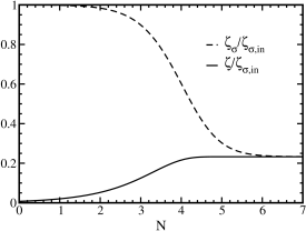
Figure 2: Evolution of the normalised curvature perturbation on uniform curvaton density hypersurfaces, $\zeta_{\sigma}/\zeta_{\sigma,{\rm in}}$, and of the normalised total curvature perturbation, $\zeta/\zeta_{\sigma,{\rm in}}$, as a function of the number of e-foldingss, starting with $\zeta_{\sigma}/\zeta_{\sigma,{\rm in}}=1$ and initial density and decay rate $\Omega_{\sigma}=10^{-2}$ and $\Gamma/H=10^{-3}$.

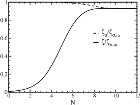
Figure 3: Evolution of the normalised curvature perturbation on uniform curvaton density hypersurfaces, $\zeta_{\sigma}/\zeta_{\sigma,{\rm in}}$, and of the normalised total curvature perturbation, $\zeta/\zeta_{\sigma,{\rm in}}$, as a function of the number of e-foldingss, starting with $\zeta_{\sigma}/\zeta_{\sigma,{\rm in}}=1$ and initial density and decay rate $\Omega_{\sigma}=10^{-2}$ and $\Gamma/H=10^{-6}$.

Figure 4: Transfer parameter $r$ defined in Eq. (71) obtained from numerical solutions as a function of the initial value of $\Omega_{\sigma}/(\Gamma/H)^{1/2}$.

III.3 Comparison with sudden decay approximation

Previous analyses curvaton ; Bozza ; LUW have relied on the assumpton of “sudden decay” to estimate the final curvature perturbation produced after curvaton decay. In this approximation the energy transfer $Q_{\sigma}=-\Gamma\rho_{\sigma}$ is assumed to be negligible until the decay time, defined by $\Gamma/H$ reaching some critical value $\Gamma/H_{\rm dec}$ of order unity, at which time all the energy density of the curvaton field is rapidly converted into radiation.

In the absence of energy transfer the individual curvature perturbations $\zeta_{\sigma}$ and $\zeta_{\gamma}$, defined by Eq.(20), remain constant on large scales [see Eq. (33)]. Thus the total curvature perturbation, Eq. (21), is given by

$$\zeta\approx f\zeta_{\sigma}+(1-f)\zeta_{\gamma}\,,$$ (74)

where $\zeta_{\sigma}$ and $\zeta_{\gamma}$ are constant and the only time dependence arises from the time dependence of the weight given to the curvaton perturbation

$$f\equiv{3\Omega_{\sigma}\over 3\Omega_{\sigma}+4\Omega_{\gamma}}\,.$$ (75)

After the curvaton decays into radiation all the energy density in the model has a unique equation of state, hence $\delta P_{\rm nad}=0$ in Eq. (26), and $\zeta$ becomes constant on large scales. Hence in the curvaton scenario, where the initial curvature perturbation $\zeta_{\gamma}$ is assumed to be negligible, the resulting adiabatic curvature perturbation after curvaton decay is given by

$$\zeta_{\rm out}\approx f_{\rm dec}\zeta_{\sigma,{\rm in}}\,.$$ (76)

In terms of an initial value for $\Omega_{\sigma,{\rm in}}$ and reduced decay rate $\Gamma/H_{\rm in}$, we can write $f_{\rm dec}$ as

$$f_{\rm dec}\equiv{3\Omega_{\sigma,{\rm in}}\over 3\Omega_{\sigma,{\rm in}}+4(1-\Omega_{\sigma,{\rm in}})y_{\rm dec}}\,,$$ (77)

where $y_{\rm dec}=a_{\rm in}/a_{\rm dec}$ is the ratio of initial scale factor to that at decay. We can calculate this from the Friedmann equation for non-interacting matter and radiation which can be written as

$$\left({H\over H_{\rm in}}\right)^{2}=(1-\Omega_{\sigma,{\rm in}})\left({a_{\rm in}\over a}\right)^{4}+\Omega_{\sigma,{\rm in}}\left({a_{\rm in}\over a}\right)^{3}\,.$$ (78)

Thus the epoch of decay, $y_{\rm dec}$, is given by the one real root, $0<y_{\rm dec}<1$ of

$$(1-\Omega_{\sigma,{\rm in}})y_{\rm dec}^{4}+\Omega_{\sigma,{\rm in}}\,y_{\rm dec}^{3}-\left(\frac{\Gamma/H_{\rm in}}{\Gamma/H_{\rm dec}}\right)^{2}=0\,,$$ (79)

and $f_{\rm dec}$ is then obtained from Eq. (77).

There are two limiting cases:

$$f_{\rm dec}\approx\left\{\begin{array}[]{ll}{3\over 4}\Omega_{\sigma,{\rm in}}(1-\Omega_{\sigma,{\rm in}})^{-3/4}\left({\Gamma/H_{\rm dec}\over\Gamma/H_{\rm in}}\right)^{1/2}&\quad{\rm for}\ y_{\rm dec}\gg\Omega_{\sigma,{\rm in}}/(1-\Omega_{\sigma,{\rm in}})\\ 1-{4\over 3}\Omega_{\sigma,{\rm in}}^{-4/3}(1-\Omega_{\sigma,{\rm in}})\left({\Gamma/H_{\rm dec}\over\Gamma/H_{\rm in}}\right)^{1/2}&\quad{\rm for}\ y_{\rm dec}\ll\Omega_{\sigma,{\rm in}}/(1-\Omega_{\sigma,{\rm in}})\end{array}\right.\,.$$ (80)

The sudden decay approximation is compared with numerical results for the full equations (65) and (66) in Figure 5. The one free parameter in the sudden-decay approximation is the particular value of $\Gamma/H_{\rm dec}$ chosen to characterise the epoch of decay. Optimising the fit to the full numerical solutions fixes $\Gamma/H_{\rm dec}\simeq 1.4$, in line with our expectation that $\Gamma/H_{\rm dec}$ should be of order unity. With this choice the sudden-decay approximation is seen (Figure 5) to give a good estimate for $r\simeq f_{\rm dec}$ (good to within 10%).

Figure 5: Comparison of full numerical solution for $r$ in Eq. (73) with sudden-decay approximation, $f_{\rm dec}$ given in Eq. (77).

IV Conclusions

We have studied the evolution of large-scale curvature perturbations for multiple interacting fluids in a linearly perturbed FRW cosmology. The curvature perturbation, $\zeta_{\alpha}$, on hypersurfaces of uniform density for each fluid, Eq. (20), provides a gauge-invariant variable by which to study the large-scale evolution. The total curvature perturbation, $\zeta$, is then a weighted sum, Eq. (21), of the individual $\zeta_{\alpha}$’s. For a non-interacting perfect fluid, $\zeta_{\alpha}$ remains constant on large scales, independently of perturbations in other fluids WMLL . More generally we have shown how $\zeta_{\alpha}$ can change on large scales due to either an intrinsic non-adiabatic pressure perturbation or non-adiabatic energy transfer.

We can decompose an arbitrary energy transfer perturbation into two parts:

$$\delta Q_{\alpha}={\dot{Q}_{\alpha}\over\dot{\rho}_{\alpha}}\delta\rho_{\alpha}+\delta Q_{\alpha,{\rm intr}}\,,$$ (81)

where $\delta Q_{\alpha,{\rm intr}}$ is the (gauge-invariant) intrinsic non-adiabatic energy transfer. The large-scale curvature perturbation $\zeta_{\alpha}$ can change due to this intrinsic non-adiabatic energy transfer, or due to a relative entropy perturbation between fluids, $\delta Q_{\alpha,{\rm rel}}$ defined in Eq. (36), which is proportional to $\zeta_{\alpha}-\zeta$. For perturbations that obey the generalised adiabatic condition:

$$\delta P_{\alpha}=c_{\alpha}^{2}\delta\rho_{\alpha}\,,\ \ \delta Q_{\alpha}={\dot{Q}_{\alpha}\over\dot{\rho}_{\alpha}}\delta\rho_{\alpha}\,\ \ {\rm and}\ \ \zeta_{\alpha}=\zeta\,,$$ (82)

the curvature perturbation, $\zeta_{\alpha}$, remains constant on large scales. If all the individual fluids obey this generalised adiabatic condition, then the total curvature perturbation, $\zeta$, is necessarily constant too.

Most previous analyses have adopted the variables of Kodama and Sasaki KS who defined the relative entropy perturbation between two fluids as

$${S}_{\alpha\beta}\equiv{\delta\rho_{\alpha}\over\rho_{\alpha}+P_{\alpha}}-{\delta\rho_{\beta}\over\rho_{\beta}+P_{\beta}}\,.$$ (83)

However this definition is only gauge-invariant in the absence of energy transfer. As a result the evolution equations including energy transfer are particularly unpleasant KS ; hama . In particular it is diffcult to show that entropy perturbations obey a homogeneous evolution equation on large scales (i.e., adiabatic perturbations stay adiabatic on large scales) in the way that was recently shown for multiple interacting scalar fields chris . Although it has been be argued on very general grounds that this must be the case WMLL , this fundamental result has not previously been explicitly demonstrated in treatments of interacting fluids.

We have used the correct gauge-invariant generalisation of (83), allowing for energy transfer,

$${\cal{S}}_{\alpha\beta}\equiv 3(\zeta_{\alpha}-\zeta_{\beta})\,,$$ (84)

which describes the relative displacement between the two hypersurfaces of uniform density defined with respect to the two fluids. This reduces to (83) in the case of no energy transfer. It allows us to demonstrate that the evolution of the large-scale entropy perturbation, Eq. (39) is sourced only by entropy perturbations and not sourced by the total curvature perturbation, $\zeta$. Thus the integrated evolution on large scales, even when we include energy transfer, can be schematically represented by the linear transfer matrix:

$$\left(\begin{array}[]{c}\zeta\\ {\cal{S}}\end{array}\right)_{\rm out}=\left(\begin{array}[]{cc}1&T_{\zeta{\cal{S}}}\\ 0&T_{{\cal{S}}{\cal{S}}}\end{array}\right)\left(\begin{array}[]{c}\zeta\\ {\cal{S}}\end{array}\right)_{\rm in}\,.$$ (85)

We have applied our formalism to study the evolution of curvature perturbations in the curvaton scenario where an initially isocurvature (non-adiabatic) perturbation in the curvaton field is transferred to the radiation fluid when the curvaton eventually decays. The decay of the curvaton represents a non-adiabatic energy source for the radiation fluid. We have numerically solved the coupled evolution equations to determine the resulting curvature perturbation, $\zeta$, for an initial entropy perturbation. Thus we have calculated the transfer coefficient $T_{\zeta{\cal{S}}}$ in Eq. (85) for different parameter values of the background models. We compared our results with semi-analytic estimates based on the “sudden-decay” approximation curvaton ; LUW where the fluids are assumed to be non-interacting up until a fixed decay time. The sudden-decay approximation is shown to give a good fit to the full result (within 10%) for a suitable choice of fitting parameter.

In this two-fluid realisation of the curvaton scenario the interaction between the fluids leads to the relative entropy decaying to zero at late times, $T_{{\cal{S}}{\cal{S}}}=0$ in Eq. (85), leaving a purely adiabatic curvature perturbation. Our formalism can also be applied to cosmological models including other cosmological fluids such as baryons, CDM or neutrinos, in which case it should be possible to calculate the amplitude of any residual isocurvature perturbations that may survive after curvaton decay in different variations of the curvaton scenario.

- (1) J. M. Bardeen, Phys. Rev. D 22 (1980) 1882.
- (2) J. M. Bardeen, P. J. Steinhardt and M. S. Turner, Phys. Rev. D 28, 679 (1983).
- (3) J. M. Bardeen, DOE/ER/40423-01-C8 Lectures given at 2nd Guo Shou-jing Summer School on Particle Physics and Cosmology, Nanjing, China, Jul 1988.
- (4) V. N. Lukash, Sov. Phys. JETP 52(5), 807 (1980) (Zh. Eksp. Teor. Fiz. 79, 1601 (1980)).
- (5) D. H. Lyth, Phys. Rev. D 31 (1985) 1792.
- (6) V. F. Mukhanov, H. A. Feldman and R. H. Brandenberger, Phys. Rept. 215 (1992) 203.
- (7) D. Wands, K. A. Malik, D. H. Lyth and A. R. Liddle, Phys. Rev. D 62 (2000) 043527 [astro-ph/0003278].
- (8) S. Mollerach, Phys. Rev. D 42 (1990) 313.
- (9) J. Garcia-Bellido and D. Wands, Phys. Rev. D 53, 5437 (1996) [arXiv:astro-ph/9511029].
- (10) D. Polarski and A. A. Starobinsky, Nucl. Phys. B 385, 623 (1992).
- (11) A. A. Starobinsky and J. Yokoyama, arXiv:gr-qc/9502002.
- (12) M. Sasaki and E. D. Stewart, Prog. Theor. Phys. 95, 71 (1996) [arXiv:astro-ph/9507001].
- (13) V. F. Mukhanov and P. J. Steinhardt, Phys. Lett. B 422, 52 (1998) [arXiv:astro-ph/9710038].
- (14) D. Polarski and A. A. Starobinsky, Phys. Rev. D 50, 6123 (1994) [arXiv:astro-ph/9404061].
- (15) A. D. Linde and V. Mukhanov, Phys. Rev. D 56, 535 (1997) [arXiv:astro-ph/9610219].
- (16) D. Langlois, Phys. Rev. D 59, 123512 (1999) [arXiv:astro-ph/9906080].
- (17) C. Gordon, D. Wands, B. A. Bassett and R. Maartens, Phys. Rev. D 63 (2001) 023506 [arXiv:astro-ph/0009131].
- (18) K. Enqvist and M. S. Sloth, Nucl. Phys. B 626, 395 (2002) [arXiv:hep-ph/0109214].
- (19) D. H. Lyth and D. Wands, Phys. Lett. B 524, 5 (2002) [arXiv:hep-ph/0110002].
- (20) T. Moroi and T. Takahashi, Phys. Lett. B 522, 215 (2001) [Erratum-ibid. B 539, 303 (2002)] [arXiv:hep-ph/0110096]; Phys. Rev. D 66, 063501 (2002) [arXiv:hep-ph/0206026].
- (21) D. H. Lyth, C. Ungarelli and D. Wands, Phys. Rev. D 67, 023503-1-13 (2003) [arXiv:astro-ph/0208055].
- (22) H. Kodama and M. Sasaki, Prog. Theor. Phys. Suppl. 78 (1984) 1.
- (23) T. Hamazaki and H. Kodama, Prog. Theor. Phys. 96 (1996) 1123, gr-qc/9609036.
- (24) H. Kodama and M. Sasaki, Int. J. Mod. Phys. A 1 (1986) 265.
- (25) H. Kodama and M. Sasaki, Int. J. Mod. Phys. A 2 (1987) 491.
- (26) J. c. Hwang and H. Noh, Class. Quant. Grav. 19, 527 (2002) [arXiv:astro-ph/0103244]. Phys. Rev. D 64 (2001) 103509 [arXiv:astro-ph/0108197].
- (27) M. Bastero-Gil, V. Di Clemente and S. F. King, hep-ph/0211011.
- (28) P. K. Dunsby, M. Bruni and G. F. Ellis, Astrophys. J. 395, 54 (1992).
- (29) Y. Nambu and A. Taruya, Class. Quant. Grav. 15, 2761 (1998) [arXiv:gr-qc/9801021]; Y. Nambu and S. i. Ohokata, Class. Quant. Grav. 19, 4263 (2002) [arXiv:gr-qc/0207019].
- (30) E. Gessner and H. Dehnen [astro-ph/0204277]
- (31) N. Bartolo, S. Matarrese and A. Riotto, Phys. Rev. D 64, 083514 (2001) [arXiv:astro-ph/0106022]; Phys. Rev. D 64, 123504 (2001) [arXiv:astro-ph/0107502]; Phys. Rev. D 65, 103505 (2002) [arXiv:hep-ph/0112261].
- (32) A. Notari and A. Riotto, Nucl. Phys. B 644, 371 (2002) [arXiv:hep-th/0205019].
- (33) F. Di Marco, F. Finelli and R. Brandenberger, arXiv:astro-ph/0211276.
- (34) P. R. Ashcroft, C. van de Bruck and A. C. Davis, arXiv:astro-ph/0210597.
- (35) J. c. Hwang and H. Noh, Phys. Lett. B 495, 277 (2000) [arXiv:astro-ph/0009268].
- (36) B. J. van Tent and S. Groot Nibbelink, arXiv:hep-ph/0111370.
- (37) K. A. Malik, arXiv:astro-ph/0101563.
- (38) M. S. Turner, Phys. Rev. D 28 (1983) 1243.
- (39) V. Bozza, M. Gasperini, M. Giovannini and G. Veneziano, Phys. Lett. B 543, 14 (2002) [arXiv:hep-ph/0206131].