Selection of Metal-poor Giant Stars Using the Sloan Digital Sky Survey Photometric System

List of spectroscopically observed giant candidates

Abstract

We present a method for photometric selection of metal-poor halo giants from the imaging data of the Sloan Digital Sky Survey (SDSS). These stars are offset from the stellar locus in the $g-r$ vs. $u-g$ color-color diagram. Based on a sample of 29 candidates for which spectra were taken, we derive a selection efficiency of the order of 50%, for stars brighter than $r\sim 17^{m}$. The candidates selected in 400 deg² of sky from the SDSS Early Data Release trace the known halo structures (tidal streams from the Sagittarius dwarf galaxy, the Draco dwarf spheroidal galaxy), indicating that such a color-selected sample can be used to study the halo structure even without spectroscopic information. This method, and supplemental techniques for selecting halo stars, such as RR Lyrae stars and other blue horizontal branch stars, can produce an unprecedented three-dimensional map of the Galactic halo based on the SDSS imaging survey.

1 Introduction

Studies of the Galactic halo can help constrain the formation history of the Milky Way. Currently popular hierarchical models of galaxy formation predict the presence of substructures (tidal tails, streams) due to the mergers and accretion the Galaxy may have experienced over its lifetime (Helmi et al. 2002; Steinmetz & Navarro 2002). These structures should be ubiquitous in the outer halo, where the dynamical timescales are sufficiently long for them to remain spatially coherent (Johnston et al. 1996; Mayer et al. 2002). The best tracers of the outer halo are the luminous giant stars (which can be detected at distances of over 100 kpc), and several investigations are taking advantage of tailored techniques, like Washington photometry (Geisler 1984), to identify these stars (e.g. Majewski et al. 2000; the Spaghetti Photometric Survey (SPS), see Morrison et al. 2000). In previous works blue horizontal branch and RR Lyrae stars also have been used to probe the outer halo (Sommer-Larsen et al. 1994; Kinman et al. 1994), and even discover substructures, many of which are debris from the Sagittarius dwarf galaxy (Ivezić et al. 2000; Yanny et al. 2000; Vivas et al. 2001).

The Sloan Digital Sky Survey (SDSS; York et al. 2000) has the potential of revolutionizing studies of the Galactic halo because it will provide homogeneous and deep ($r<22.5$) photometry in five passbands ($u$, $g$, $r$, $i$, and $z$, Fukugita et al. 1996; Gunn et al. 1998; Smith et al. 2002; Hogg et al. 2002) accurate to a few percent of up to 10,000 deg² in the Northern Galactic Cap. The survey sky coverage will result in photometric measurements for about 50 million stars and a similar number of galaxies. Astrometric positions are accurate to better than 0.1 arcsec per coordinate (rms) for sources brighter than 20.5^m (Pier et al. 2002). Such a large database is well suited for studies of Galactic structure, with the caveat that the photometric system must be able to identify different classes of stars, and variations in their metallicity and luminosity. This separation is particularly challenging for Galactic halo tracers, because the number of halo stars at a given magnitude is much smaller than that of any other Galactic component (e.g. in a high-latitude field at $b=45^{\circ}$, at $V\sim 17^{m}$ and $0.3\leq(B-V)\leq 1.5$ the fraction of halo giants is $\sim 6$%, cf. Robin et al. 2000).

In this paper, we present a method designed to select candidate metal-poor giants based on their SDSS colors. Using a sample of known metal-poor halo giants discovered by the Spaghetti Survey, we isolated a region in the SDSS $g-r$ vs. $u-g$ color-color diagram where the probability of a star being a giant is enhanced. Spectroscopic observations of an unbiased sample of 29 “candidate” stars with $r<17$ indicate that the selection efficiency of our technique is approximately 50%. In Section §2 we describe the selection method, and in Section §3 we discuss its implications for the Galactic halo studies.

2 Color Selection of Metal-poor Giant Stars

2.1 The SDSS Photometric Data

We use SDSS imaging data that were taken during the commissioning phase, and which are part of the SDSS Early Data Release (Stoughton et al. 2002, hereafter EDR). We analyze here equatorial observing runs 94, 125, 752 and 756 which include two regions: $|\,\delta_{2000}|\lesssim 1.27^{\circ}$, and $\alpha_{2000}=$ 23^h 24^m – 03^h 44^m (runs 94 and 125), and $\alpha_{2000}=$08^h 7^m – 16^h 40^m (runs 752 and 756), and cover 394 deg². In order to test the photometric repeatability, we also use run 1755 which overlaps with run 125 in the range $\alpha_{2000}=$ 23^h 22^m – 03^h 03^m (74.8 deg² area). Note that the wide range of Galactic coordinates implies that the different Galactic components will manifest themselves with varying strength within this dataset.

We have extracted 2,143,248 objects classified as point sources by the photometric pipeline (photo, Lupton et al. 2001), which do not have any of the following flags set: bright, satur, blended, notchecked, deblended_as_moving. This flag combination selects sources with the most reliable photometry (for details see EDR and Ivezić et al. in prep., hereafter Paper II). We use the “point-spread function” magnitudes corrected for interstellar reddening (Schlegel et al. 1998).

2.2 SDSS Colors of the Spaghetti Giants

Some regions observed by the Spaghetti survey overlap with runs 752 and 756. The SPS’s Washington photometry is used to isolate metal-poor stars on the basis of their $(M-T_{2})$ and $(M-51)$ colors (sensitive to temperature and the strength of the Mg$b$ and MgH features near 5200 Å, respectively, cf Geisler et al. 1991; Paltoglou & Bell 1994), and to obtain a first estimate of the luminosity class of the stars. These candidates are observed spectroscopically, and are classified into dwarfs and giants using the following indicators (Morrison et al. 2002):

• the Mg$b$ and MgH features near 5200 Å, which are characteristic of dwarfs, and are almost absent in giant stars for $0.8\leq(B-V)\leq 1.3$ (Flynn & Morrison 1990);

• the CaI $\lambda$4227 line, which is usually present in dwarfs and absent in giants. While this feature may be visible in metal-poor giants (with [Fe/H]$\geq-1.5$), it is much weaker than in dwarfs of the same color;

• the CaII H and K lines near 3950 Å, which are sensitive to [Fe/H] (cf Beers et al. 1999).

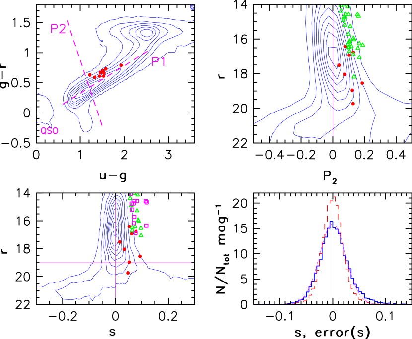
Figure 1: The top left panel shows with contours the distribution of 19,000 stars with $r$$<$19 in the $g-r$ vs. $u-g$ color-color diagram. A sample of metal-poor giants discovered by the Spaghetti survey is shown by solid circles (all panels); note that they are offset from the locus center. The dashed lines show a principal axes system aligned with the locus. The top right panel shows the $r$ vs. $P_{2}$ color-magnitude diagram, and the bottom left panel shows the $s$ vs. $P_{2}$ diagram, where $s$ is derived from $P_{2}$ by accounting for the magnitude dependence. The thick solid histogram in the bottom right panel shows the distribution of the $s$ color for stars brighter than $r=19$ from run 125, that were also observed in run 1755. The dashed histogram shows the $s$ error distribution determined from multiple observations. The thin solid curve is a best Gaussian fit to the $s$ color distribution and shows that the latter is not symmetric: the red wing has more stars than the blue wing. The candidate giants from the spectroscopic sample discussed in Sec. 3.2 are shown by triangles in the upper right panel, and divided into confirmed giants (squares) and dwarfs (triangles) in the bottom left panel.

The contours in the top left panel in Fig. 1 show, in the $g-r$ vs. $u-g$ color-color diagram, the distribution of 19,000 stars from run 125 that are brighter than $r=19$ and whose photometric errors in all bands ($u$, $g$, $r$) are less than 0.05. Nine SPS giants (Dohm-Palmer et al. 2001) are shown by filled circles and are clearly offset from the center of the stellar locus (for a discussion of the position of the stellar locus in the SDSS photometric system see e.g. Finlator et al. 2000). In the other SDSS color-color projections the SPS giants fall right on the stellar locus, having $0.15\leq\hbox{$r-i$}\leq 0.4$ and $0\leq\hbox{$i-z$}\leq 0.25$. Note also that since metal-poor stars are bluer than metal-rich stars of the same temperature (cf Mihalas & Binney 1981), they are shifted left from the main locus in the $g-r$ vs. $u-g$ diagram shown in Fig. 1 (Lenz et al. 1998; Fan 1999).

2.3 Definition of the $s$ Color

We use the well-defined stellar locus to derive a principal axes coordinate system ($P_{1}$, $P_{2}$), where $P_{1}$ lies parallel to the stellar locus and $P_{2}$ measures the distance from it (see also Odenkirchen et al. 2001; Willman et al. 2001). The origin is chosen to coincide with the highest stellar density ($u-g$$=1.21$, $g-r$$=0.42$). Since the objects of interest occur in a relatively narrow color range, we restrict ourselves to $1.1\leq\hbox{$u-g$}\leq 2$ and $0.3\leq\hbox{$g-r$}\leq 0.8$ (we refer the reader to Lenz et al. 1998 for an extensive study on how the SDSS colors of stars translate into temperature, metallicity and surface gravity). This procedure yields:

$$\hbox{$P_{1}$}=0.910\,(\hbox{$u-g$})+0.415\,(\hbox{$g-r$})-1.28,$$ (1)

$$\hbox{$P_{2}$}=-0.415\,(\hbox{$u-g$})+0.910\,(\hbox{$g-r$})+0.12.$$ (2)

The top right panel in Fig. 1 shows the $r$ vs. $P_{2}$ color-magnitude diagram for 47,771 stars from run 125. The position of the locus clearly depends on the $r$ magnitude (the median $P_{2}$ color becomes redder at the faint end), and we correct for this effect using a linear $P_{2}$ vs. $r$ fit (the correction varies from –0.03 to 0.05 mag). We thus define a new color, $s$ – named after the Spaghetti survey–, that is normalized such that its error is approximately equal to the mean photometric error in a single band (assuming uncorrelated measurements in the $u$, $g$, and $r$ bands). We obtain

$$s=-0.249\,u+0.794\,g-0.555\,r+0.24.$$ (3)

The $r$ vs. $s$ color-magnitude diagram for stars with $-0.1<\hbox{$P_{1}$}<0.6$ is shown in the bottom left panel in Fig. 1. The thick solid line in the bottom right panel in Fig. 1 shows the distribution of the $s$ color for stars brighter than $r=19$ that were observed both in runs 125 and 1755. The equivalent Gaussian distribution width determined from the interquartile range is 0.035 mag. The dashed line shows the distribution of the difference in the $s$ color between the two epochs divided by $\sqrt{2}$; its width is 0.025 mag; that is, the error distribution is narrower than the observed $s$ color distribution, demonstrating that the $s$ color distribution reflects some intrinsic stellar property. The thin solid line is a best Gaussian fit to the $s$ color distribution and shows that the latter is not symmetric: the red wing contains more stars than the blue wing.

2.4 The Selection Criteria for Metal-poor Giants

Based on the $s$ color distribution of the Spaghetti giants and the overall $s$ color distribution, we select candidate metal-poor giants as stars with $r<19$ and $-0.1<\hbox{$P_{1}$}<0.6$ (for $1.1\leq\hbox{$u-g$}\leq 2$ and $0.3\leq\hbox{$g-r$}\leq 0.8$) and

$$s>m_{s}+0.05,$$ (4)

where $m_{s}$ is the median value of $s$ color in appropriately chosen subsamples. Since the accuracy of EDR data calibration is finite (about 0.01–0.02 mag), $m_{s}$ is not exactly zero. We calibrate independently the data corresponding to a given run and camera column (i.e. individual scanline), and compute $m_{s}$ for these subsamples. As expected, the $m_{s}$ distribution is well described by a Gaussian with a width of $\sim$0.025 mag (see top right panel of Fig. 2). Note as well that $m_{s}$ (or equivalently the location of the principal axes) may change slightly as a function of Galactic coordinates as a result of a different mixture of stellar populations. However, this shift is sufficiently small that we may neglect it. Hereafter, we will simply use $\hat{s}$ when referring to this median-corrected color.

3 Tests of the Selection Method

3.1 Comparisons of the candidates and a control sample

We define two samples for comparing the angular and magnitude distribution: the “candidates” R with $\hat{s}>+0.05$, and the “control sample” B with $\hat{s}<-0.05$. In all runs that we have analyzed, we find that the number of stars in R is significantly larger than in B. We compare the angular and magnitudes distribution of the two samples in Fig. 2 for stars in runs 752 and 756 whose photometric errors in all bands ($u$,$\,g$,$\,r$) are less than 0.05. To account for a smaller number of stars in B  we have selected a random subset of R having the same size as B.

The top left panels in Fig. 2 show that the angular distribution of stars in R appears more isotropic than that of B. In particular, the number of stars in B increases toward lower Galactic latitudes, indicating that they are dominated by the disk population. It is evident from the bottom left panels in the same Figure that the samples have different magnitude distributions – the R sample contains a larger fraction of bright stars –, which possibly reflects different distance distributions. These results hint toward an overall different spatial distribution for stars in the “candidate region” from those in the “control sample”. The bottom right panel shows that there is an enhancement in the stellar density of the R sample (dotted curve) for $\alpha_{2000}$ in the range $13^{h}-16^{h}$, which can be linked to the recently discovered clumps in the Galactic Halo, associated with the Sagittarius dwarf northern tidal streams (Ivezić et al. 2000; Yanny et al. 2000; Dohm-Palmer et al. 2001; Martinez-Delgado et al. 2001; Newberg et al. 2002). We performed a $\chi^{2}$ statistical test to determine the probability that the B and R samples are drawn from the same parent population. If we restrict the samples to $\alpha_{2000}=13^{h}-16^{h}$, we find this probability to be $\sim 3\times 10^{-9}$. If no restriction is applied the probability is even smaller $\sim 10^{-10}$. The southern streams of Sagittarius in runs 94 and 125 ($\alpha_{2000}\sim 1^{h}15^{m}$, $\delta_{2000}\sim 0^{\circ}$; Yanny et al. 2000), and the Draco dwarf spheroidal galaxy in runs 1336/9 and 1356/9 ($\alpha_{2000}=17^{h}20^{m}$, $\delta_{2000}=57.9^{\circ}$; Odenkirchen et al. 2001), – none of which is shown in Fig. 2 – are recovered as clear overdensities in the distribution of “candidate stars”, which is not the case for stars in the “control sample”.

3.2 Spectroscopic Observations and Analysis

The results from the previous subsection suggest that the fraction of halo giants in the candidate subset R is significantly larger than that of the comparison sample B. To investigate this, and to derive an estimate of the selection efficiency, we selected stars from two overlapping runs 125 and 1755 which satisfy the selection criteria in both runs. Of a total of 72 candidates with $\hat{s}>0.05$, we randomly selected 29, for which we obtained intermediate resolution spectra. The data reduced with the most recent version of photometric pipeline (photo v5_3) have photometric errors of the order 0.02 mag, smaller than the EDR data used here which have errors of the order 0.03 mag. The requirement that the candidate stars qualify in both runs has a similar effect on efficiency as smaller photometric errors, and thus the selection efficiency obtained here is more representative of the upcoming SDSS Data Release 1.

The $r$ magnitudes of the selected candidates range from 14 to 17, with a median $r$ magnitude of $16$ (see Table 1 for the list of stars and their colors). The spectra were obtained during the nights of October 20–24 2001, using CAFOS on the Calar Alto 2.2m telescope in the framework of the “Calar Alto Key Project for SDSS Follow-up Observations” (Grebel 2001). The resolution was 4 Å, the spectral range $\lambda=3200-5800$ Å, and we integrated each star for 900 up to 2000 seconds depending on the brightness of the star and weather conditions. The reduction process will be described in detail in Paper II.

In the wavelength range probed by the selection method, the features most sensitive to luminosity class are those used by the SPS: the Mg$b$ triplet near 5170Å and the CaI $\lambda$4227 line. In Fig. 3 we show the spectra of six of the stars in the program. With the obtained resolution and signal-to-noise ratios, it is possible to separate the giants from the dwarfs even by simple visual inspection. The three spectra in the left panels clearly show the absence of the MgH and Mg$b$ triplet (compare to the spectra shown in the right panel), thus proving that at least some of the stars in our sample are giants. To obtain a more quantitative discrimination between giant and dwarf stars, we also measure the equivalent widths of the CaII K, the CaI $\lambda$4227 and the Mg$b$ triplet lines, according to the definitions by Morrison et al. (2002). We use their calibrations to assign luminosity class. Out of the 29 observed stars, 12 are metal-poor giants, 13 are metal-poor dwarfs, and for 4 stars the obtained signal-to-noise ratio is insufficient for classification. A rough estimate of [Fe/H] has been obtained by visual inspection of the spectra (we do not have enough standards for proper calibration). Such a method has an inherent uncertainty of about 0.5 dex.

We conclude that the identification of metal-poor giants can be done with satisfactory efficiency, of order 50%, using the SDSS photometric data. However, we caution that stars in our spectroscopic sample are relatively bright ($r<17$), and thus this efficiency will be lower than 50% for fainter magnitudes due to increased photometric errors and contamination by subdwarfs.

4 Discussion

The technique described in this Letter can be used to study the structure of the Galactic halo in two complementary ways. One method is to select candidates for spectroscopic follow-up and determine their luminosity class and radial velocity. The latter essentially adds an extra dimension which could prove useful to disentangle structures in the halo (Harding et al. 2001). This approach would be analogous to that used by the SPS. A second possibility, and which makes perhaps a better use of the uniquely large SDSS dataset, is a statistical approach. One can compare the angular and magnitude distributions of candidate giant stars with that of stars in a “control sample”, in the same spirit of Fig. 2. A statistical subtraction of the distributions of the datasets may allow, for example, a mapping of overdensities in the number of candidate giant stars at different locations in the sky. When combined with other techniques for selecting halo stars, such as RR Lyrae stars and blue horizontal branch stars, it will be possible to produce an unprecedented detailed three-dimensional map of the Galactic halo based on the SDSS imaging survey.

Figure 2: The panels on the left show the sky distribution (declination vs. right ascension $\alpha$) and $r$ magnitude vs. $\alpha$ diagrams for stars in runs 752 and 756 satisfying Eq.(4). There are 5125 stars in R and 2844 in B . Here we have selected a random sample of R with the same number of stars as in B for a more direct comparison of the spatial distribution of stars in each subset. The regions $\alpha\lesssim 10^{h}$ and $15.5^{h}\lesssim\alpha$ contain data from a driftscan that does not have interleaving stripes, hence the very uneven distribution of stars at different declinations in those regions. The top right panels show the median $s$-color and the dispersion as a function of $\alpha$ for the six independent camera columns. We have excluded data closer than 150 pixels to the chip edge, because the flatfielding uncertainties in the $u$ band increase photometric errors by about 1%. The histograms in the bottom right panel show the number of stars per 2.5 deg. bins for the whole R sample (dotted curve), for the B sample (dashed curve) and for a random realization of the R sample with the same number of stars as B (solid curve).

Figure 3: Spectra of six “candidate stars”, which were observed with the 2.2m telescope at Calar Alto. The spectra have 4 Å resolution, and have not been flux calibrated. The panels on the left show the spectra of three giants, while those on the right correspond to three dwarfs. Notice the strong Mg$H$ and Mg$b$ triplet in the dwarfs, which are almost absent in the giants. The “candidate stars” have characteristic colors with median($g-r$) $=$ 0.62, which typically corresponds to a $T_{eff}\sim 5000K$, median($u-g$) $=$ 1.40, and median($s$) $=$ 0.07. Their median $r$ magnitude is 16.03.

$\alpha_{2000}~{}~{}(^{h}~{}^{m}~{}^{s})$	$\delta_{2000}~{}~{}(^{\circ}~{}^{\prime}~{}^{\prime\prime})$	$u-g$	$g-r$	$r$	$s$	“class”
23 22 49.9	45.6	1.18	0.52	14.57	0.08	G
23 23 30.5	58 17.9	1.47	0.75	16.35	0.12	G
23 23 44.0	30 16.9	1.32	0.64	14.59	0.12	G
23 25 51.1	1     0 23.0	1.62	0.79	17.06	0.10	D
23 28 57.0	55 49.8	1.56	0.50	16.31	0.06	u
23 29 16.7	55 51.4	1.31	0.61	16.89	0.08	G
23 31  $\,\,5.9$	2 21.7	1.47	0.66	15.27	0.08	D
23 31 22.3	$-$17 32.4	1.33	0.59	16.45	0.07	u
23 34 59.6	$-$16   5.1	1.40	0.62	15.72	0.07	G
23 37 35.1	$-$1     5   2.5	1.71	0.77	16.68	0.07	D
23 43 56.4	10 52.3	1.35	0.58	14.58	0.07	G
23 49 39.7	$-$42 57.0	1.70	0.77	16.42	0.07	D
23 51 53.9	2 37.9	1.60	0.71	16.71	0.06	D
4 56.7	$-$18 37.0	1.07	0.54	14.67	0.12	G
5  $\,\,7.3$	2 40.8	1.37	0.62	15.94	0.09	D
10 16.9	52 25.4	1.71	0.71	14.05	0.06	G
15 24.1	$-$21 26.9	1.38	0.69	16.25	0.11	u
21 57.5	$-$17 38.5	1.23	0.52	14.75	0.07	G
29  $\,\,0.8$	5 29.5	1.42	0.59	14.77	0.06	G
30  $\,\,5.8$	$-$24   7.2	1.62	0.78	16.53	0.10	D
32 20.1	51 41.4	1.09	0.48	16.17	0.07	G
32 31.5	$-$22 27.2	1.61	0.72	16.47	0.06	D
33 36.4	$-$49   8.7	1.42	0.57	14.38	0.06	D
33 40.5	$-$17 17.5	1.42	0.62	14.13	0.08	D
34 28.4	32   4.3	1.47	0.69	16.03	0.09	D
35 44.5	4 12.4	1.30	0.54	15.19	0.06	G
38 21.8	$-$17 48.4	1.35	0.56	14.02	0.07	D
38 39.2	7 12.9	1.64	0.69	14.91	0.06	D
38 42.4	35 55.1	1.23	0.55	16.11	0.07	u

Table 1: Right ascension, declination, apparent magnitudes and colors of the 29 candidates with follow$-$up spectra. The last column denotes whether the star is a giant (G), dwarf (D) or whether the spectra was not good enough to determine the luminosity class (u).

References

- Beers et al. (1999) Beers, T. C., Rossi, S., Norris, J. E., Ryan, S. G., & Shefler, T. 1999, AJ, 117, 981
- Dohm-Palmer et al. (2001) Dohm-Palmer, R.C., et al. 2001, ApJ, 555, L37
- Fan (1999) Fan, X. 1999, AJ, 117, 2528
- Finlator (2000) Finlator, K., et al. 2000, AJ, 120, 2615
- Flynn & Morrison (1990) Flynn, C. & Morrison, H. L. 1990, AJ, 100, 1181
- Fukugita et al. (1996) Fukugita, M., Ichikawa, T., Gunn, J. E., Doi, M., Shimasaku, K., & Schneider, D. P. 1996, AJ, 111, 1748
- Geisler (1984) Geisler, D., 1984, PASP, 96, 723
- Geisler, Claria, & Minniti (1991) Geisler, D., Claria, J. J., & Minniti, D. 1991, AJ, 102, 1836
- (9) Grebel, E. K., 2001, Reviews in Modern Astronomy, 14, 223
- (10) Gunn, J.E., et al. 1998, AJ, 116, 3040
- Harding et al. (2001) Harding, P., Morrison, H. L., Olszewski, E. W., Arabadjis, J., Mateo, M., Dohm-Palmer, R. C., Freeman, K. C., & Norris, J. E. 2001, AJ, 122, 1397
- Helmi et al. (2002) Helmi, A., White, S.D.M., & Springel, V., 2002, MNRAS in press, astro-ph/0208041
- (13) Hogg, D.W., Finkbeiner, D.W., Schlegel, D.W., & Gunn, J.E. 2002, AJ, 122, 2129
- Ivezic et al (2000) Ivezić, Ž. et al. 2000, AJ, 120, 963
- Johnston et al. (1996) Johnston, K.V., Hernquist, L., & Bolte, M., 1996, ApJ, 465, 278
- Kinman, Suntzeff, & Kraft (1994) Kinman, T. D., Suntzeff, N. B., & Kraft, R. P. 1994, AJ, 108, 1722
- (17) Lenz, D. D., Newberg, H. J., Rosner, R., Richards, G. T., & Stoughton, C. 1998, ApJS, 119, 121
- (18) Lupton, R.H. et al. 2001, in Astronomical Data Analysis Software and Systems X, ASP Conf. Proc., Vol.238, p. 269. eds. F.R. Harnden, Jr., F. A. Primini, & H. E. Payne
- Majewski, Ostheimer, Kunkel, & Patterson (2000) Majewski, S. R., Ostheimer, J. C., Kunkel, W. E., & Patterson, R. J. 2000, AJ, 120, 2550
- Martinez-Delgado, Aparicio, Gómez-Flechoso, & Carrera (2001) Martinez-Delgado, D., Aparicio, A., Gómez-Flechoso, M.A., & Carrera, R. 2001, ApJ, 549, L199
- Mayer et al. (2002) Mayer, L., Moore, B., Quinn, T., Governato, F., & Stadel, J., 2002, MNRAS, 336, 119
- Mihalas & Binney (1981) Mihalas, D. & Binney J., 1981, “Galactic Astronomy”, Freeman, p. 120
- Morrison et al. (2000) Morrison, H.L., et al. 2000, AJ, 119, 2254
- Morrison et al. (2001) Morrison, H. L., Olszewski, E. W., Mateo, M., Norris, J. E., Harding, P., Dohm-Palmer, R. C., & Freeman, K. C. 2001, AJ, 121, 283
- Morrison et al. (2002) Morrison, H.L., et al. 2002, submitted to AJ
- Newberg et al. (2002) Newberg, H. J., Yanny, B., Rockosi, C., et al., 2002, ApJ, 569, 245
- Odenkirchen et al. (2001) Odenkirchen, M. et al., 2001, AJ, 122, 2538
- Paltoglou & Bell (1994) Paltoglou, G. & Bell, R. A. 1994, MNRAS, 268, 793
- Pier et al. (2002) Pier, J.R., et al. 2002, AJ, in press
- Robin et al. (2000) Robin, A. C., Reylé, C., Crézé, M., 2000, A&A, 359, 103
- Schlegel, Finkbeiner, & Davis (1998) Schlegel, D. J., Finkbeiner, D. P., & Davis, M. 1998, ApJ, 500, 525
- (32) Smith, J.A., et al. 2002, AJ, 123, 2121
- Sommer-Larsen, Flynn, & Christensen (1994) Sommer-Larsen, J., Flynn, C., & Christensen, P. R. 1994, MNRAS, 271, 94
- Steinmetz & Navarro (2002) Steinmetz, M. & Navarro, J. F. 2002, New Astronomy, 7, 155
- Stoughton et al. (2002) Stoughton, C. et al. 2002, AJ, 123, 485
- Vivas et al. (2001) Vivas, A. K. et al. 2001, ApJ, 554, L33
- Yanny et al (2000) Yanny, B. et al. 2000, ApJ, 540, 825
- (38) York, D.G. et al. 2000, AJ, 120, 1579
- Willman et al. (2002) Willman, B., Dalcanton, J., Ivezić, Ž., Jackson, T., Lupton, R., Brinkmann, J., Henessy, G., Hindsley, R., 2002, AJ, 123, 848