Low-Frequency Gravitational Waves from Massive Black Hole Binaries: Predictions for LISA and Pulsar Timing Arrays

Abstract

The coalescence of massive black hole (BH) binaries due to galaxy mergers provides a primary source of low-frequency gravitational radiation detectable by pulsar timing measurements and by the proposed LISA (Laser Interferometry Space Antenna) observatory. We compute the expected gravitational radiation signal from sources at all redshifts by combining the predicted merger rate of galactic halos with recent measurements of the relation between BH mass, $M_{\rm bh}$, and the velocity dispersion of its host galaxy, $\sigma$. Our main findings are as follows: (i) the nHz frequency background is dominated by BH binaries at redshifts $z\lesssim 2$, and existing limits from pulsar timing data place tight constraints on the allowed normalization and power-law slope of the $M_{\rm bh}$–$\sigma$ relation or on the fraction of BH binaries that proceed to coalescence; (ii) more than half of all discrete mHz massive BH sources detectable by LISA are likely to originate at redshifts $z\gtrsim 7$; (iii) the number of LISA sources per unit redshift per year should drop substantially after reionization as long as BH formation is triggered by gas cooling in galaxies. Studies of the highest redshift sources among the few hundred detectable events per year, will provide unique information about the physics and history of black hole growth in galaxies.

1 Introduction

A future detection of gravitational waves (GWs) will not only test the theory of General Relativity, but will also provide a precious new tool in astronomy (Hughes et al. 2001, and references therein). This tool will be particularly effective for studying compact objects because the information carried by GWs is very different from that of electromagnetic radiation. Gravitational radiation is generated by different physical processes and is often emitted from dense regions that are otherwise hidden from traditional astronomical observations. A very important distinction, particularly for the study of the distant universe is that while the usual observable for electromagnetic radiation is an energy flux which drops in proportion to distance squared, the direct observable for gravitational radiation is the wave amplitude $h$ which drops off only as distance. As a result, the coalescence of many massive black-hole (BH) binaries ($M_{\rm bh}>10^{3}M_{\odot}$) will be detectable by the planned GW observatory LISA (Laser Interferometry Space Antenna) at mHz frequencies out to very high redshifts (Haehnelt 1994; Hughes et al. 2001). At the lower $\mu$Hz frequencies, pulsar timing measurements limit the level of the cosmic GW background, contributed mainly by the early phase in the coalescence of massive BH binaries (Kaspi et al. 1994; Thorsett & Dewey 1996; Lommen 2002).

Massive BH binaries are among the primary sources for LISA. Such binaries are produced by mergers of galaxies with pre-existing black holes, provided that coalescence due to the interaction of the binary with its surrounding galaxy occurs in less than a Hubble time. Hughes (2002) has shown that LISA observations of the gravitational radiation during both the inspiral and ring-down phases of massive BH binary coalescence can be used to determine the source redshift, while the source position on the sky can be inferred within a fraction of an orbit of the LISA satellite. Recently, Seto (2002) has noted that consideration of the finite length of the LISA detector leads to significant improvements in estimations of the accuracy to which the three-dimensional positions for coalescing BH binaries can be measured.

Black holes are ubiquitous in low redshift galaxies (e.g. Magorrian et al. 1998). Their masses, $M_{\rm bh}$, as determined from dynamical measurements (e.g. Merritt & Ferrarese 2001; Tremaine et al. 2002) or from reverberation mapping of AGN (e.g. Ferrarese et al. 2001; Laor 2001), correlate tightly with the velocity dispersion, $\sigma_{\star}$, of their host stellar bulge. However, the abundance of massive BHs in galaxies at high redshifts is not well known. In fact, Menou, Haiman & Narayanan (2001) have argued that an occupation fraction as low as 0.01 at redshift 5 can result through subsequent mergers, in all local massive galaxies containing massive BHs. Nevertheless, one might expect massive BHs to be ubiquitous at high redshifts for the following reason. It is commonly thought that present day BHs are the dormant remnants of the active galactic nuclei observed at high redshift. Recent observations of this population have reached out beyond redshift 6 (Fan et al. 2001). The quasars discovered are very bright, and must be powered by BH masses of $\gtrsim 10^{9}$M_⊙. Recent modeling by Wyithe & Loeb (2002) has shown that the density of these high-redshift quasars as well as lower redshift populations can be explained through merger activity using the same relation between host velocity dispersion and BH mass as observed locally. The latter assumption is supported by the recent observation that the relation between velocity dispersion and BH mass holds in quasars out to redshift 3 (Shields et al. 2002). This result suggests that if BHs are not ubiquitous in galaxies at high redshift, then it must be a coincidence that the active quasar period increases at high redshift in inverse proportion to the occupation fraction. Note also that the inferred active period for a BH at $z\sim 6$ is $\sim 10^{7}$yr or $\sim 1\%$ of a Hubble time (Wyithe & Loeb 2002). Thus the minimum occupation fraction at $z\sim 6$ is $\sim 0.01$.

The emission of GWs requires that the binary coalesce in less than a Hubble time. What is the mechanism that brings a wide binary system with an orbital separation $\gtrsim 1$ kpc into the regime where coalescence is dominated by gravitational radiation? Several mechanisms have been discussed in the literature, including dynamical friction on the background stars (e.g. Begelman, Blandford, & Rees 1980; Rajagopal & Romani 1995; Milosavljevic & Merritt 2001; Yu 2002), and a gas dynamical effect analogous to that thought responsible for planetary migration (Gould & Rix 2000; Armitage & Natarajan 2002). Yu (2002) has followed the expected evolution of massive central BH binaries in a sample of nearby early-type galaxies for which high-resolution photometry exists, and found that the evolution timescale increases significantly when the BH binary becomes hard before entering the GW regime. Spherical galaxies often lead to coalescence timescales that are longer than a Hubble time, while highly flattened or triaxial galaxies lead to faster coalescence. Regardless of the physical mechanism, Haehnelt & Kauffmann (2002) argue that if central binaries do not merge in less than a Hubble time, then three-body interactions resulting from subsequent mergers will cause ejection and too much scatter in the $M_{\rm bh}-\sigma_{\star}$ relation. Hereafter, we assign an efficiency $\epsilon_{\rm mrg}$ to the coalescence process. Throughout this paper we show numerical results under the assumption that BH binaries formed through the merger of two galaxies proceed quickly to coalescence ($\epsilon_{\rm mrg}=1$), but point out the relevant scaling with $\epsilon_{\rm mrg}$ where appropriate.

The number of binary sources depends on a convolution over redshift of the merger rate of galaxies with the fraction of galaxies that harbor massive BHs. Several attempts have been made to compute the event rate (Fukushige, Ebisuzaki & Makino 1992; Haehnelt 1994; Rajagopal & Romani 1995; Haehnelt 1998; Menou, Haiman & Narayanan 2002; Jaffe & Backer 2002), either based on observational counts of quasars and elliptical galaxies with arbitrary extrapolations to higher redshift, or using merger tree algorithms based the Press-Schechter theory. Despite the fact that detectors such as LISA are expected to detect events at exceedingly high redshift, many calculations have only considered low ($z<5$) redshift sources. However, recent evidence of bright quasar activity at $z\sim 6$ (Fan et al. 2001) and independent evidence that these quasars reside in massive dark-matter halos (Barkana & Loeb 2002), suggests that BHs might be as ubiquitous at the centers of high-redshift galaxies as they are today. Furthermore, prior to reionization the ability of gas to cool inside small halos is mainly limited by the efficiency of gas cooling rather than by the infall of gas from a heated and photoionized intergalactic medium, and so massive BHs could form inside much smaller galaxies than are available after reionization (e.g. Barkana & Loeb 2000; Haiman, Abel & Rees 2001; Thoul & Weinberg 1996). As a result it is possible that a substantial fraction of the events detectable by LISA have originated prior to reionization. Our paper explores this possibility.

Recently, Jaffe & Backer (2002) have computed the spectrum of characteristic strain resulting from massive BH mergers in the $n$Hz-$\mu$Hz regime using a phenomenological approach for the merger rate and BH mass function up to some maximum redshift. They found that the logarithmic spectral slope of the stochastic cosmic background of gravitational radiation that results from inspiraling BHs is -2/3, independent of the details of their model for the merger rate and BH mass function. This provides a numerical confirmation of the general result derived by Phinney (2001). They also found that the amplitude of the spectrum is close to the limit probed by recent pulsar timing experiments, but is sensitive to the model assumed for the BH mass function and merger rate. In this paper we make a full semi-analytic calculation of the entire merger rate history starting from the highest redshifts when the first galaxies are believed to have formed in the universe (Barkana & Loeb 2001, and references therein). We employ the formalisms of Press & Schechter (1974) and Lacey & Cole (1993), and compute the resulting redshift-dependent BH mass function (including the effect of reionization) using the observed relation between BH mass and halo circular velocity. We compare our results with current limits on the cosmic GW background at low frequencies, and extend the calculation upwards in frequency to the LISA band.

Throughout the paper we assume density parameter values of $\Omega_{m}=0.35$ in matter, $\Omega_{b}=0.052$ in baryons, $\Omega_{\Lambda}=0.65$ in a cosmological constant, and a Hubble constant of $H_{0}=65~{}{\rm km\,s^{-1}\,Mpc^{-1}}$ (or equivalently $h=0.65$). For calculations of the Press-Schechter (1974) mass function (with the modification of Sheth & Tormen 1999) we assume a primordial power-spectrum with a power-law index $n=1$ and the fitting formula to the exact transfer function of Cold Dark Matter, given by Bardeen et al. (1986). Unless otherwise noted we adopt a present-day rms amplitude of $\sigma_{8}=0.87$ for mass density fluctuations in a sphere of radius $8h^{-1}$Mpc.

The paper is organized as follows. In § 2 we describe calculation of the evolution of the BH mass-function following reionization. In § 4, § 5 and § 6 we use the results of this calculation to predict the merger rate and hence the detection rate of GW sources by LISA, the distribution of event durations, and the resulting spectrum of the characteristic strain. Finally, we present our conclusions in § 7.

2 Evolution of the Mass-Function of Halos Hosting Massive Black Holes

During hierarchal galaxy formation, an average property of the galaxy population, such as the density of galaxies evolves in redshift due to newly collapsing halos, mergers of halos and accretion. In this section we discuss the calculation of the rate of newly collapsing halos, and then demonstrate a method to calculate the continuous evolution of the massive BH mass function.

Let $\frac{dn_{\rm ps}}{dM}(z)$ be the Press-Schechter mass function (number of halos with mass between $M$ and $M+dM$ per co-moving Mpc) of dark-matter halos at a redshift $z$. We include the extension of Sheth & Tormen (1999) which improves the agreement with direct numerical simulations (Jenkins et al. 2001). The rate of change (with respect to redshift) of the density of dark matter halos with masses between $M_{1}$ and $M_{1}+dM_{1}$ is therefore $\frac{d^{2}n_{\rm ps}}{dM_{1}dz}$. Let us also define $\frac{d^{2}N_{\rm mrg}}{d\Delta Mdt}\left.\right|_{M}$, the number of mergers per unit time of halos of mass $\Delta M$ with halos of mass $M$ (forming new halos of mass $M_{1}=M+\Delta M$) at redshift $z$ (Lacey & Cole 1993).

We consider mergers of halos having masses greater than $M_{\rm min}=100M_{\odot}$. Addition of mass from halos smaller than $M_{\rm min}$ is treated as smooth accretion. In what follows this contribution to the growth of halos must be included to maintain a self-consistent calculation. We therefore find the component of the change in the density of halos with masses between $M_{1}$ and $M_{1}+dM_{1}$ that is due to accretion rather than to mergers. This is given by the overall change in the density of halos with mass $M_{1}$, minus the change due to merger of halos to form a new halo of mass $M_{1}$, plus the change in density of halos of mass $M_{1}$ that merge with other halos (a change that was compensated for in the net $\frac{d^{2}n_{\rm ps}}{dM_{1}dz}$). The net change in density of halos of mass $M_{1}$ through accretion is then,

$$\frac{d^{2}n_{\rm acc}}{dM_{1}dz}=\frac{d^{2}n_{\rm ps}}{dM_{1}dz}-\int_{M_{\rm min}}^{\frac{M_{1}}{2}}d\Delta M\left.\frac{d^{2}N_{\rm mrg}}{d\Delta Mdt}\right|_{M_{1}-\Delta M}\frac{dt}{dz}\frac{dn_{\rm ps}}{d(M_{1}-\Delta M)}+\int_{M_{\rm min}}^{\infty}d\Delta M\left.\frac{d^{2}N_{\rm mrg}}{d\Delta Mdt}\right|_{M_{1}}\frac{dt}{dz}\frac{dn_{\rm ps}}{dM_{1}}.$$ (1)

We are interested in the evolution of the mass function of dark-matter halos that contain a massive BH. Prior to reionization, the minimum mass halo inside of which gas can cool is limited by the cooling rate, and corresponds to a virial temperature above $T_{\rm min}\sim 10^{4}$K if the gas cools through transitions in atomic hydrogen, or above $T_{\rm min}\sim 10^{2.4}$K if the gas cools through transitions in molecular hydrogen (Haiman, Abel & Rees 2000). Following reionization, the IGM is heated to $\sim 10^{4}$K. The Jeans mass is increased by several orders of magnitude, and numerical simulations find that gas infall is suppressed in larger halos. There is some uncertainty about the precise value of the halo circular velocity below which gas infall is suppressed (e.g. Thoul & Weinberg 1996; Kitayama & Ikeuchi 2000; Quinn, Katz & Efstathiou 1996, Weinberg, Hernquist & Katz 1997; Navarro & Steinmetz 1997). We assume that following reionization, gas can cool inside newly collapsing halos if their virial temperatures are higher than $T_{\rm min}=10^{5}$K. We denote by $F_{\rm acc}$ the fraction of halos which contain a massive BH after crossing the cooling threshhold through accretion.

Halos forming via mergers are assumed to contain a massive BH if one of the subunits used to make them already contained a BH. In addition, if the merger product has a mass larger than $M(T_{\rm min})$, then a BH could form out of the gas that cools inside the merger product. We assume that this happens in a fraction $F_{\rm mrg}$ of cases where neither the initial nor the accreted halo contained a BH. The mass function of halos containing a massive BH ($\frac{dn_{\rm bh}}{dM}$) therefore evolves according to the following differential equation:

$$\frac{d^{2}n_{\rm bh}}{dM_{1}dz} = F_{\rm acc}\frac{d^{2}n_{\rm acc}}{dM_{1}dz}\Theta[M_{1}-M(T_{\rm min})]$$ (2)

$$+ \int_{M_{\rm min}}^{\frac{M_{1}}{2}}d\Delta M\left.\frac{d^{2}N_{\rm mrg}}{d\Delta Mdt}\right|_{M_{1}-\Delta M}\frac{dt}{dz}\frac{dn_{\rm bh}}{d(M_{1}-\Delta M)}\Theta[M(T_{\rm min})-M_{1}]$$

$$+ \int_{M_{\rm min}}^{\frac{M_{1}}{2}}d\Delta M\left.\frac{d^{2}N_{\rm mrg}}{d\Delta Mdt}\right|_{M_{1}-\Delta M}\frac{dt}{dz}\left\{\left[1-\left(1-\frac{dn_{\rm bh}/d\Delta M}{dn_{\rm ps}/d\Delta M}\right)\left(1-F_{\rm mrg}\right)\right]\right.$$

$$\left.\times\left(\frac{dn_{\rm ps}}{d(M_{1}-\Delta M)}-\frac{dn_{\rm bh}}{d(M_{1}-\Delta M)}\right)+\frac{dn_{\rm bh}}{d(M_{1}-\Delta M)}\right\}\Theta[M_{1}-M(T_{\rm min})]$$

$$- \int_{M_{\rm min}}^{\infty}d\Delta M\left.\frac{d^{2}N_{\rm mrg}}{d\Delta Mdt}\right|_{M_{1}}\frac{dt}{dz}\frac{dn_{\rm bh}}{dM_{1}},$$

where $\Theta$ is the Heaviside step function. If $F_{\rm acc}=F_{\rm mrg}=1$, this equation maintains a density of BHs in halos larger than $M(T_{\rm min})$ that is equal to the Press-Schechter density. In the above equation, the first term gives the change in the density of halos containing BHs due to newly collapsing halos above the threshold virial temperature. The second and third terms give the increase due to mergers of the density of halos of mass $M_{1}$ that contain a BH. The second term gives the increase for halos below the threshold temperature due to mergers with a halo already containing a BH. This term will be important since the mass corresponding to the minimum temperature increases with time, and because reionization results in an increase of the minimum mass halo inside which gas can collapse and cool. The third term gives the increase in the density of halos with virial temperatures above the threshold temperature that contain BHs. There are two parts to this term. If the halo of mass $M_{1}-\Delta M$ contains a black hole, then so does the merger product. However if the halo of mass $M_{1}-\Delta M$ does not contain a BH then the merger product only contains a BH if one of the following two conditions hold: either the accreted halo (of mass $\Delta M$) already contained a BH, or if it did not then a BH forms in a fraction $F_{\rm mrg}$ of merger products. Finally, the fourth term allows for the loss in the density of halos of mass $M_{1}$ that contain black holes due to mergers forming a larger halo. There are two limiting cases; $F_{\rm acc}=F_{\rm mrg}=1$ in which case all galaxies with masses above the cooling threshhold contain black-holes, and $F_{\rm acc}=F_{\rm mrg}=0$ in which case the number of massive BHs drops with time through galaxy mergers. Below we discuss these cases in more detail.

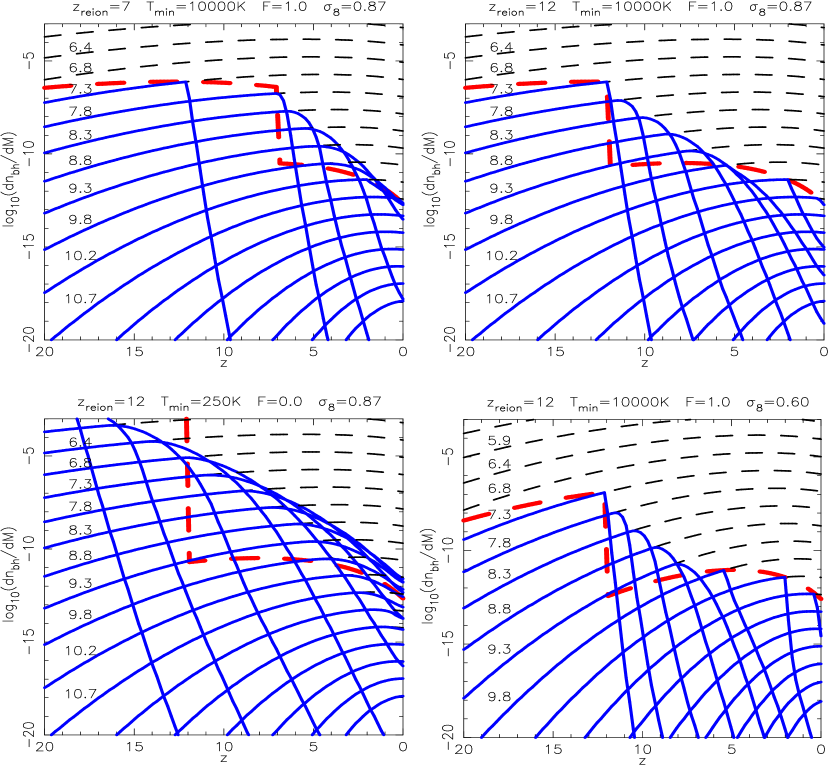
Figure 1: Solid lines: The mass function of halos that contain BHs as a function of redshift for various masses (labeled by $\log_{10}(M/M_{\odot})$). Dashed lines: The Press-Schechter mass function of halos as a function of redshift for various masses. The panels show cases I-IV whose primary parameters are listed at the top of each plot. The thick dashed line shows the density corresponding to $T_{\rm min}$ as a function of redshift.

We consider 4 examples for the evolution of $\frac{dn_{\rm bh}}{dM_{1}}$. These will be referred to throughout the paper and are labeled $I-IV$. In each case the initial values for the mass function of halos containing BHs is chosen to be

$$\frac{dn_{\rm bh,ini}}{dM_{1}}=F_{\rm ini}\frac{dn_{\rm ps}}{dM_{1}}\Theta[M_{1}-M(T_{\rm min})].$$ (3)

• (I) Begin at $z=20$ with BHs in all halos having $T_{\rm vir}>10^{4}$K, and assume $F_{\rm ini}=F_{\rm acc}=F_{\rm mrg}=1$. Reionization is assumed to be at $z_{\rm reion}=7$.

• (II) Begin at $z=20$ with BHs in all halos having $T_{\rm vir}>10^{4}$K, and assume $F_{\rm ini}=F_{\rm acc}=F_{\rm mrg}=1$. Reionization is assumed to be at $z_{\rm reion}=12$.

• (III) Begin at $z=20$ with BHs in all halos having $T_{\rm vir}>10^{2.4}$K, and assume $F_{\rm ini}=1$ and $F_{\rm acc}=F_{\rm mrg}=0$.

• (IV) Begin at $z=20$ with BHs in all halos having $T_{\rm vir}>10^{4}$K, and assume $F_{\rm ini}=F_{\rm acc}=F_{\rm mrg}=1$. Reionization is assumed to be at $z_{\rm reion}=12$, but in difference from case II , we use $\sigma_{8}=0.6$ rather than the fiducial value of $\sigma_{8}=0.87$.

Cases I, II and IV refer to situations where cooling in neutral gas is limited by atomic hydrogen, and in which BH formation is ongoing. Case III refers to situations where cooling in neutral gas is limited by molecular hydrogen, and in which the BH population arises from “seed BHs” at $z=20$.

We show the four examples of evolution of $\frac{dn_{\rm bh}}{dM}$ in Figure 1. Here the density of halos of mass $M$ that contain a BH is plotted as a function of redshift (solid lines). The dashed lines show the corresponding Press-Schechter mass function, and each pair of curves is labeled by the logarithm of the mass in $M_{\odot}$ on the left of the plot. The thick dashed line is the density of halos with the minimum virial temperature into which gas can collapse, and has a discontinuity at $z_{\rm reion}$. In cases I and II we see that following reionization, the density of halos below the critical virial temperature that contain BHs drops as these halos merge to form more massive halos. By redshift 2 ($z_{\rm reion}=7$) and 5 ($z_{\rm reion}=12$), there are no halos containing BHs left with temperatures below $T_{\rm min}$.

2.1 The Black-Hole Mass Function

The calculation of the BH mass function from the mass-function of halos that contain BHs requires specification of a relation between the BH and halo mass. Ferrarese (2002) has found a tight, power-law correlation in nearby galaxies between the mass of a dark-matter halo and the mass of its central BH. Following Haehnelt, Natarajan & Rees (1998) and Wyithe & Loeb (2002) we generalise to higher redshifts assuming a BH mass that scales as a powerlaw with circular velocity $M_{\rm bh}\propto v_{\rm c}^{\gamma}$. Using the expression for halo mass $M$ as a function of $v_{\rm c}$ (Barkana & Loeb 2001) we find

$$M_{\rm bh}=10^{12}\epsilon_{0}\left(\frac{M}{10^{12}M_{\odot}}\right)^{\gamma/3}\left(\frac{\Omega_{\rm m}}{\Omega_{\rm m}^{\rm z}}\frac{\Delta_{\rm c}}{18\pi^{2}}\right)^{\gamma/6}h^{\gamma/3}(1+z)^{\gamma/2},$$ (4)

where $\Delta_{\rm c}=18\pi^{2}+82d-39d^{2}$, $d=\Omega_{\rm m}^{\rm z}-1$ and $\Omega_{\rm m}^{\rm z}={\Omega_{\rm m}(1+z)^{3}}/[{\Omega_{\rm m}(1+z)^{3}+\Omega_{\Lambda}}]$. In this notation, the relation found by Ferrarese (2002) for BHs in the local universe has $\epsilon_{0}=10^{-5.06}$ and $\gamma=5.46$. In the remainder of the paper masses with the subscript _bh a subscript refer to BH masses, while those without refer to halo masses. The merger rates are computed in terms of halo masses, but many expressions implicitly contain conversion from BH to halo mass or vice versa using equation (4).

Simple considerations of the regulation of BH growth by feedback from quasar activity result in $\gamma=5$ (Haehnelt, Natarajan & Rees 1998; Silk & Rees 1998). Supporting this argument is the recent finding of Shields et al. (2002) that the $M_{\rm bh}-\sigma_{\star}$ relation derived from QSOs shows no redshift dependence. The growth of BHs only through hierarchical mergers imply $\gamma=3$. A value of $\gamma>3$ is therefore required in order to allow BH growth through accretion that must accompany quasar activity. With $\gamma=5$, theoretical luminosity functions require $\epsilon_{0}=10^{-5.4}$ (Wyithe & Loeb 2002), and these are the values used throughout this work unless specified otherwise. The mass function of BHs is therefore

$$\frac{dn_{\rm bh}}{dM_{\rm bh}}=\frac{dn_{\rm bh}}{dM}\frac{3}{\gamma}\frac{M}{M_{\rm bh}}.$$ (5)

Figure 2: The mass functions of massive BHs at various redshifts. The panels show cases I-IV whose primary parameters are listed at the top of each plot.

The evolution of $\frac{dn_{\rm bh}}{dM_{\rm bh}}$ is shown in each of cases I-IV in Figure 2. The mass-function of halos that contain BHs $\left(\frac{dn_{\rm bh}}{dM}\right)$ is insensitive to the BH–halo mass relation. However, in the examples shown, BHs exist in halos as small as $M\lesssim 10^{8}M_{\odot}$. Extrapolation of the $M_{\rm bh}-v_{\rm c}$ relation down to these small galaxies is not justified by observations; moreover, it yields BH masses comparable to those expected from stars where the formation physics is very different. We therefore only show the mass function down to $M_{\rm bh}=10^{3}M_{\odot}$. We will show that the low frequency GW signal is dominated by BHs in galaxies with $M\gtrsim 10^{12}M_{\odot}$; however BHs in smaller galaxies are important as seeds for massive BHs in larger galaxies at later times.

The BH mass functions can be compared with those presented in Figure 5 of Kauffmann & Haehnelt (2000). The density of the most massive BHs increases monotonically with time, while in cases I, II and IV there is little evolution in the density of lower mass BHs before reionization. However following reionization, there is rapid evolution at low masses since newly formed low-mass halos do not produce BHs, and the density of low mass halos that contain BHs drops as they merge to form larger halos. Case III shows a different evolution; since there is no ongoing BH formation the reionization redshift does not leave any signature. Case IV with a smaller value of $\sigma_{8}=0.6$ yields lower BH densities at all redshifts.

3 Gravitational Waves from Inspiraling Binary Black-Holes

As described earlier, we assume that in a fraction $\epsilon_{\rm mrg}$ of galaxy mergers the resulting binary BHs evolve rapidly into the regime where energy loss is dominated by gravitational radiation. Defining this time as $t_{\rm start}$, the subsequent evolution of the binary is then described by equation (6). It can be shown (e.g. Shapiro & Teukolsky 1983) that the evolution in the binaries’ (circular) orbital frequency $f$ with time $t$ obeys the relation

$$t(f)-t_{\rm start}=\frac{5}{256}\frac{c^{5}}{G^{5/3}}\frac{(M_{\rm bh}+\Delta M_{\rm bh})^{1/3}}{M_{\rm bh}\Delta M_{\rm bh}}\left(2\pi\right)^{-8/3}\left(f_{\rm start}^{-8/3}-f^{-8/3}\right),$$ (6)

where $f_{\rm start}$ is the orbital frequency at time $t_{\rm start}$. Throughout the paper we assume circular orbits for which the observed gravitational radiation has a characteristic frequency

$$f_{\rm c}=2\frac{f}{1+z},$$ (7)

and characteristic strain, averaged over orientations and polarizations (Thorne 1987) of

$$h_{\rm c}=8\left(\frac{2}{15}\right)^{1/2}\frac{G^{5/3}M_{\rm bh}\Delta M_{\rm bh}}{c^{4}R(z)(M_{\rm bh}+\Delta M_{\rm bh})^{1/3}}\left(2\pi f\right)^{2/3},$$ (8)

where $R(z)$ is the co-moving coordinate distance to redshift $z$. The choice of $R(z)$ as the distance measure ensures that the energy flux, which is proportional to $(h_{\rm c}f_{\rm c})^{2}$, declines in proportion to the inverse square of the luminosity distance. As a binary loses energy, the frequency as well as amplitude of the gravitational radiation increase with time. Following Hughes (2002) we assume that the inspiral attains its maximum frequency when the two BHs are separated by 3 Schwarzschild radii, i.e. $f_{\rm max}=c^{3}/(2\pi 6^{3/2}GM)$Hz for a Schwarzschild BH, and stop our calculation at this point. Hughes & Blandford (2002) find that following a major merger, the remnant is rarely rotating rapidly unless the mass ratio is $\sim 1$. In this work we neglect the subsequent higher frequency radiation from the coalescence and ringdown phases.

4 The Merger Rate and the Counts of Gravitational Wave Sources

The proposed GW observatory LISA will be able to detect many mergers of massive BHs out to very high redshifts (Haehnelt 1994; Hughes et al. 2001). It is therefore interesting to calculate the number of detectable mergers expected per unit redshift per unit (observed) time on the sky. Previous attempts at this calculation have used empirical local rates and extrapolation (e.g. Backer & Jaffe 2002), or have used a merger tree algorithm. Menou, Haiman & Narayanan (2001) used a merger tree algorithm to predict the merger rate out to $z\sim 5$, beyond which they found that the Press-Schechter mass function was no longer accurately recovered. We have circumvented this problem by integrating the BH mass function forward in time, while exactly preserving the Press-Schechter mass function. This allows us to explore the merger rate at higher redshifts and identify the possible signature of reionization in GW observations.

Figure 3: The rate of GW events per unit redshift, per observed year. The panels show cases I-IV whose primary parameters are listed at the top of each plot. We assume $\epsilon_{0}=10^{-5.4}$ and $\gamma=5$. For comparison the dashed line shows the event rate where $T_{\rm min}$ is assumed not to rise following reionization.

The number of detectable BH mergers per observed year per unit redshift across the entire sky is

$$\frac{d^{2}N_{\rm gw}}{dtdz} = \int_{0}^{\infty}dM\int_{0}^{M}d\Delta M\;\Theta(M,\Delta M,f_{\rm c},h_{\rm c},z)\times S(z,M_{\rm bh},\Delta M_{\rm bh})$$

$$\times\left.\frac{d^{2}N_{\rm mrg}}{d\Delta Mdt}\right|_{M}\frac{dn_{\rm bh}}{dM}\left[\frac{dn_{\rm bh}/d\Delta M}{dn_{\rm ps}/d\Delta M}\right]\frac{\epsilon_{\rm mrg}}{1+z}4\pi\frac{d^{2}V}{dzd\Omega},$$

where $V$ is the co-moving volume and $\Omega$ is solid angle on the sky. Note that there must be BHs present in both galaxies in order for gravitational radiation to be produced (this being the origin of the term in square brackets). The function $\Theta(M,\Delta M,f_{\rm c},h_{\rm c},z)$ has a value of 1 if the merger produces a detectable strain in the LISA band, but is zero otherwise. In our calculations throughout this paper we set $\epsilon_{\rm mrg}=1$. Since $\epsilon_{\rm mrg}$ is our parameterization of the efficiency with which dynamical friction brings binary BHs into the GW regime, this corresponds to the assumption that all BH binaries coalesce. However, more generally, $\frac{d^{2}N_{\rm gw}}{dtdz}\propto\epsilon_{\rm mrg}$.

At a frequency of $f_{\rm c}=10^{-3}$Hz, the expected value of the threshhold sensitivity is $h_{\rm c}\sim 10^{-22}$ for a signal to noise ratio of 5 (needed for confident detection of a binary with unknown frequency and direction) and one year of observation. We find that the typical event duration at frequencies between $f_{\rm c}=10^{-3.5}$Hz and $f_{\rm c}=10^{-2.5}$Hz ranges between a few months to a year. We therefore assume detectability if the strain amplitude $h_{\rm c}>10^{-22}$ at an observed frequency of $f_{\rm c}=10^{-3}$Hz. Note that a full calculation of the signal to noise ratio of an observation requires comparison of the coherently folded signal power (including the evolution in its frequency) to the noise power accumulated over the bandwidth of the measurement. By working with the quantity $h_{c}$ (Thorne 1987), we approximately account for the detection threshold.

The function $S$ is included in equation (4) because the merger of dark matter halos does not imply the immediate merger of the stellar systems within. Colpi, Mayer & Governato (1999) have studied the evolution of satellites in virialized halos. They find that the orbital decay time is

$$t_{\rm decay}=1.2\left(\frac{r_{\rm vir}}{v_{\rm c}}\right)\frac{M+\Delta M}{\left[\frac{\Delta M}{e}\right]\mbox{ln}\left(\frac{M+\Delta M}{\Delta M}\right)}\epsilon^{0.4},$$ (10)

where $r_{\rm vir}$ is the initial radius and $\epsilon\sim 0.5$ is the circularity of the of the orbit (Ghigna et al. 1998). Note that even though $\epsilon\sim 0.5$ for the initial orbit of the secondary galaxy in the dark matter halo, eventually the eccentricity decays rapidly during the GW driven inspiral of the binary BH system (e.g. Peters 1964; Hughes & Blandford 2002; Yu 2002). The dynamical time may be written from the expressions in Barkana & Loeb (2001) as

$$\frac{r_{\rm vir}}{v_{\rm c}}=0.10H^{-1}\left[\frac{\Omega_{\rm m}}{\Omega_{\rm m}^{\rm z}}\frac{\Delta_{\rm c}}{18\pi^{2}}\right]^{-1/2}h^{-1}(1+z)^{-3/2}$$ (11)

and amounts to about a tenth of the Hubble time. In order to have the satellite sink in less than a Hubble time, the merging galaxies must be of comparable mass. The dynamical evolution of a massive binary BH may be disrupted if there is a subsequent major merger before coalescence of the initial binary. This typically leads to the ejection of the lightest of the three black-holes (e.g. Haehnelt & Kauffmann 2002; Volonteri, Haardt & Madau 2002). To account for this phenomenon in a simple way, we assume that at most one coalescence can occur during the decay time $t_{\rm decay}$ or within a Hubble time, whichever is the larger. In mergers where the satellite does not sink within a Hubble time, we assume no coalescence. Furthermore, following Kauffmann & Haehnelt (2000) we suppress gas accretion and therefore BH mergers within galaxies with $v_{\rm c}>600$km/sec, though this restriction does not significantly affect our results. We therefore include the function $S(z,M_{\rm bh},\Delta M_{\rm bh})$ which is set to $\left[\mbox{max}\left(\Delta Mt_{\rm decay}\left.\frac{d^{2}P}{d\Delta Mdt}\right|_{M},1\right)\right]^{-1}$ if the satellite galaxy’s orbital decay time $t_{\rm decay}$ is smaller than the Hubble time, $\left(H_{0}\sqrt{\Omega_{\rm m}(1+z)^{3}+\Omega_{\Lambda}}\right)^{-1}$, and if both galaxies have $v_{\rm c}<600$km/sec, but equals zero otherwise.

The quantity $\frac{d^{2}N_{\rm gw}}{dtdz}$ is plotted in Figure 3 in the case where $T_{\rm min}=10^{4}$K at all times (dashed lines) and in the cases I–IV (solid lines). The first case closely resembles the one considered by Menou et al. (2001) in which they had BHs in all halos (although they did not apply a detection limit, and hence obtained much higher event rates). The integrated event rate $N_{\rm mrg}$ is listed in each panel of Figure 3. We find that $N_{\rm mrg}$ is sensitive to the reionization redshift, with values of $N_{\rm mrg}\sim 350$yr^-1 and $N_{\rm mrg}\sim 145$yr^-1 assuming $z_{\rm reion}=7$ and $z_{\rm reion}=12$ respectively (cases I and II). As is evident from the plot, the source counts may probe the reionization epoch out to large redshifts. There is a drop in the event rate at or soon after the reionization redshift. This drop arises because even though some halos below the critical temperature still contain BHs until $z\sim 2$ ($z_{\rm reion}=7$) and $z\sim 5$ ($z_{\rm reion}=12$) respectively, the event rate scales as the square of the BH occupation fraction. Similar behavior is seen in case IV, however the smaller value of $\sigma_{8}=0.6$ suppresses the growth of structure at early times relative to our fiducial case of $\sigma_{8}=0.87$. The resulting counts are much lower than in cases I-III, $N_{\rm mrg}\sim 15$yr^-1. The drop following reionization is much larger if the suppression of gas infall extends to larger galaxies. For example, if $T_{\rm min}=2.5\times 10^{5}$K following reionization, the suppression of the number counts is more than an order of magnitude within 2 redshift units.

Similar results are found with $F_{\rm ini}=F_{\rm acc}=F_{\rm mrg}=0.01$ ($N_{\rm mrg}\sim 340$yr^-1 and $N_{\rm mrg}\sim 140$yr^-1 for cases I and II). Since mergers quickly result in massive BHs being ubiquitous in larger galaxies even if the occupation fraction is initially small (Menou, Haiman & Narayanan 2001), the number counts and the corresponding spectra (see subsequent sections) are weakly dependent on $F_{\rm ini}$, $F_{\rm acc}$ and $F_{\rm mrg}$. We therefore only consider $F_{\rm ini}=F_{\rm acc}=F_{\rm mrg}=1$ for cases I, II and IV in the remainder of this paper.

5 The Distribution of Event Durations of Gravitational Waves from Inspiraling BH Binaries

In the previous section we calculated the event rate of detectable gravitational radiation sources for the LISA satellite. However we would also like to know how long these events will last. To this end we calculate the distribution of event durations $\Delta t$ for sources having observed strains between $h_{\rm c}$ and $h_{\rm c}+\Delta h_{\rm c}$ at $f_{\rm c}=10^{-3}$Hz. We define the event duration $\Delta t$ as the time taken for the frequency to pass through a single decade in frequency from $f_{\rm c}=10^{-3.5}$Hz to $f_{\rm c}=10^{-2.5}$Hz.

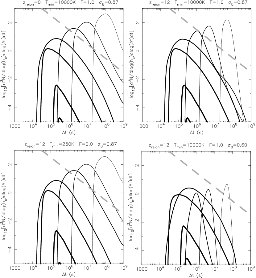
Figure 4: Plots of $\frac{d^{3}N}{d\log(h_{\rm c})d\log(\Delta t)dt}$ at different values of strain. Each panel the lines corresponding to $h_{\rm c}=10^{-23}$, $10^{-22}$, $10^{-21}$, $10^{-20}$, $10^{-19}$ and $10^{-18}$, from right to left. Also shown is the line of $3.15\times 10^{7}\mbox{sec}/\Delta t$ which approximates the confusion limit for observations with no directional information. Curves below this line correspond to radiation from distinct events. The panels show cases I-IV whose primary parameters are listed at the top of each plot. We assume $\epsilon_{0}=10^{-5.4}$ and $\gamma=5$.

To calculate the event duration distribution, we assume that a fraction $\epsilon_{\rm mrg}$ of binary BHs produced through galaxy mergers evolve rapidly into the regime where energy loss is dominated by gravitational radiation. We can use the merger rate and the mass function of halos containing massive BHs together with the BH – halo mass relation in equation (4) to find the observed number of events of duration $\Delta t$ per unit strain per year. Thus

$$\frac{d^{3}N}{dh_{\rm c}d\Delta tdt} = \int_{0}^{\infty}dM\int_{0}^{M}d\Delta M\int_{0}^{\infty}dz\frac{dn_{\rm bh}}{dM}\left.\frac{d^{2}N_{\rm mrg}}{d\Delta Mdt}\right|_{M}\left(\frac{dn_{\rm bh}/d\Delta M}{dn_{\rm ps}/d\Delta M}\right)\times 4\pi\frac{\epsilon_{\rm mrg}}{1+z}\frac{d^{2}V}{dzd\Omega}$$ (12)

$$\times\delta\left[K(M_{\rm bh},\Delta M_{\rm bh},z)\right]\delta\left[T(M_{\rm bh},\Delta M_{\rm bh},z)\right]\times S(z,M_{\rm bh},\Delta M_{\rm bh}),$$

where $\delta(x)$ is the Dirac delta function, from equation (8)

$$K(\Delta M_{\rm bh})\equiv h_{\rm c}-8\left(\frac{2}{15}\right)^{1/2}\frac{G^{5/3}M_{\rm bh}\Delta M_{\rm bh}}{c^{4}R(z)(M_{\rm bh}+\Delta M_{\rm bh})^{1/3}}\left(2\pi f\right)^{2/3},$$ (13)

and the function $S$, which was introduced in the previous section controls the fraction of galaxy mergers that can result in BH coalescence within a Hubble time. From equation (6) we find that there is a single redshift corresponding to each delay for a given combination of merging BH masses, hence

$$T(z)\equiv\Delta t-\frac{40}{256\pi^{2}}\left(\frac{2}{15}\right)^{0.5}\frac{c}{h_{\rm c}}\left(10^{-3}~{}{\rm Hz}\right)^{2/3}\left[\left(10^{-3.5}~{}{\rm Hz}\right)^{-8/3}-\left(10^{-2.5}~{}{\rm Hz}\right)^{-8/3}\right]\left[R(z)(1+z)^{2}\right]^{-1}.$$ (14)

Making the assumption that the timescale for the final inspiral is short compared with a Hubble time (in the $\epsilon_{\rm mrg}\times S$ of cases where the satellite sinks to the center of the merger product and the resulting BH binary enters the GW regime in less than a Hubble time), we can take the mass-function and merger rate terms outside the redshift integral in equation (12). If we then integrate over $\delta\left[K(M,\Delta M,z)\right]$ using $\int d\Delta M$, and over $\delta\left[T(M,\Delta M,z)\right]$ using $\int dz$ we find

$$\frac{d^{3}N}{dh_{\rm c}d\Delta tdt} =$$ (15)

$$\int_{0}^{\infty}dM\frac{dn_{\rm bh}}{dM}\left.\frac{d^{2}N_{\rm mrg}}{d\Delta Mdt}\right|_{M}\left[\Delta M_{\rm bh}=K^{-1}(0)\right]\left(\frac{dn_{\rm bh}/d\Delta M}{dn_{\rm ps}/d\Delta M}\right)\times 4\pi\frac{\epsilon_{\rm mrg}}{1+z}\frac{d^{2}V}{dzd\Omega}\times S(z,M_{\rm bh},\Delta M_{\rm bh})$$

$$\times\left(\left|\frac{dK}{d\Delta M_{\rm bh}}\left[\Delta M_{\rm bh}=K^{-1}(0)\right]\right|\frac{d\Delta M_{\rm bh}}{d\Delta M}\right)^{-1}\left(\left|\frac{dT}{dz}\left[z=T^{-1}(0)\right]\right|\right)^{-1}\Theta\left[M_{\rm bh}-K^{-1}(0)\right],$$

where we have used the relation

$$\int dx\delta\left[g(x)\right]=\int dx\sum_{i}\frac{1}{\left|\frac{dg}{dx}\left[x=g_{i}^{-1}(0)\right]\right|}\delta\left[x\right].$$ (16)

The terms are evaluated using the value of $\Delta M_{\rm bh}=K^{-1}(0)$ found by solving the cubic equation (8), which has only one positive real root. The value $z=T^{-1}(0)$ is found numerically from equation (14). The Heaviside step function $\Theta\left[M_{\rm bh}-K^{-1}(0)\right]$ ensures that mergers are not counted twice. Equation (15) has the following intuitive explanation. For each combination of $M$ and $\Delta M$ there is a merger rate to which the event rate is directly related. The derivative $\left(\frac{dK}{d\Delta M_{\rm bh}}\right)^{-1}$ relates the interval of strain to the interval of $\Delta M$, thus providing the number density of mergers $\frac{d^{2}N_{\rm mrg}}{d\Delta Mdt}d\Delta M$ producing events in $dh_{\rm c}$. Finally the derivative $\left(\frac{dT}{dz}\right)^{-1}$ relates the interval of event duration to the interval of redshift in which the source can be located. The volume in which these sources will be found is then $4\pi\frac{d^{2}V}{dzd\Omega}dz$.

Curves representing the number of sources per $\log{\Delta t}$ per $\log{h_{\rm c}}$ per year are plotted in Figure 4 as functions of $\Delta t$ for different values of $h_{\rm c}$ in cases I-IV. Also shown is the confusion limit for observations with no directional information ($3.15\times 10^{7}\mbox{sec}/\Delta t$). Note that this confusion line assumes that the detector has no angular resolution; in the case of events with locations measured to a positional accuracy $\Delta\theta$, the confusion line should be lifted by a factor $(4\pi)/(\pi\Delta\theta^{2})$. Events with values of strain corresponding to curves below this line will be distinct, while those above the line will overlap. Events with lower frequencies come preferentially from higher redshift. These longer events are more common, which is consistent with the findings in Figure 3. Events with values of strain $h_{\rm c}\sim 10^{-20}-10^{-21}$ and above will be separable. The figure suggests that in cases I-III around 10 events per year with $h_{\rm c}\sim 10^{-20}$ will be observed, with each lasting around a few days. At a larger amplitude, $h_{\rm c}\sim 10^{-19}$, about one event per year will be observed lasting less than a day. Even larger amplitude events from inspirals will be very rare. In case IV we find that the lower event rate means that only a few distinct events are expected per year at strains of $h_{\rm c}\sim 10^{-20}$ of more. Another prominent feature of case IV is the broadness of the curve for $h_{\rm c}=10^{-20}$, being dominated by sources producing the peak in number counts near $z\sim 4$ (see Figure 3).

6 The Spectrum of the Gravitational Wave Background from Inspiraling BH Binaries

LISA will be sensitive to the final in-spirals and/or ringdown phases of most massive BH mergers (Haehnelt 1994; Hughes et al. 2001). However, with the exception of the occupation fraction, the event rate does not directly carry information on properties of the BH population itself such as the slope and normalization of the BH mass-function. Individual events will yield useful information (Hughes 2002), but we might also expect the number counts of sources in frequency and strain (i.e. the time averaged number of sources per unit frequency per unit strain at a single epoch) to provide constraints on the relation between BH and halo mass.

Figure 5: Plots of $\frac{d^{2}N}{d\log(h_{\rm c})d\log(f_{\rm c})}$ at different frequencies. In each panel the thin lines (from top to bottom) correspond to $f_{\rm c}=10^{-10}$, $10^{-9}$, $10^{-8}$, $10^{-7}$, $10^{-6}$, while the thick lines correspond to $10^{-5}$, $10^{-4}$, $10^{-3}$, $10^{-2}$ and $10^{-1}$Hz. The panels show cases I-IV whose primary parameters are listed at the top of each plot. We assume $\epsilon_{0}=10^{-5.4}$ and $\gamma=5$.

In analogy with the previous section we can use the merger rate and the mass function of halos containing massive BHs together with the BH - halo mass relation to find the instantaneous, time averaged number counts that should be observed in a snapshot of the sky per unit frequency per unit strain per co-moving Mpc,

$$\frac{d^{2}\Phi}{dh_{\rm c}df_{\rm c}}(z) = \int_{0}^{\infty}dM\int_{0}^{M}d\Delta M\int_{t_{\rm start}}^{t(z)}dt\frac{dn_{\rm bh}}{dM}\left.\frac{d^{2}N_{\rm mrg}}{d\Delta Mdt}\right|_{M}\epsilon_{\rm mrg}\times S(f_{\rm c},z,M_{\rm bh},\Delta M_{\rm bh})$$ (17)

$$\times\left(\frac{dn_{\rm bh}/d\Delta M}{dn_{\rm ps}/d\Delta M}\right)\delta\left[K(M_{\rm bh},\Delta M_{\rm bh},t-t_{\rm start})\right]\delta\left[F(M_{\rm bh},\Delta M_{\rm bh},t-t_{\rm start})\right],$$

where from equation (6)

$$F(t)\equiv f_{\rm c}-\frac{2}{(1+z)}\frac{1}{2\pi}\left[\left(2\pi f_{\rm start}\right)^{-8/3}-\frac{256}{5}\frac{G^{5/3}}{c^{5}}\frac{M_{\rm bh}\Delta M_{\rm bh}}{M_{\rm bh}+\Delta M_{\rm bh}}(t-t_{\rm start})\right]^{-3/8}.$$ (18)

Three conditions are imposed on the number counts and are incorporated in the function $S$. The first requirement is that the circular velocity of the merger product be smaller than $600$km/sec. In § 4 we assumed that coalescence and the emission of GWs at $f_{\rm c}=10^{-3}$Hz would only occur where the merging secondary galaxy sinks before the next comparable merger event and in less than a Hubble time. For calculation of equation (17) we note that within the GW dominated regime there are some frequencies and mass combinations for which coalescence does not occur within a Hubble time. We therefore assume that a BH binary produced through a galaxy merger will only result in the emission of gravitational radiation at a frequency $f_{\rm c}$ if the binary coalescence as well as the prior sinking of the satellite occur before the next comparable merger event and within a Hubble time. Thus the function $S(z,M_{\rm bh},\Delta M_{\rm bh})$ is set to $\left[\mbox{max}\left(\Delta M\left[t_{\rm decay}+t(f_{\rm c})-t(f_{\rm max})\right]\left.\frac{d^{2}P}{d\Delta Mdt}\right|_{M},1\right)\right]^{-1}$ if the satellite galaxy’s orbital decay time $t_{\rm decay}$ plus the inspiral time $[t(f_{\rm c})-t(f_{\rm max})]$ is smaller than the Hubble time, and if both galaxies have $v_{\rm c}<600$km/sec, but equals zero otherwise.

As before we make the assumption that the timescale for the final inspiral is short compared with a Hubble time and take the mass-function and merger rate terms outside the time integral in equation (17). If we then integrate over $\delta\left[K(M,\Delta M,t-t_{\rm start})\right]$ using $\int d\Delta M$, and then over $\delta\left[F(M,\Delta M,t-t_{\rm start})\right]$ using $\int dt$ we find

$$\frac{d^{2}\Phi}{dh_{\rm c}df_{\rm c}}(z) = \int_{0}^{\infty}dM\frac{dn_{\rm bh}}{dM}\left.\frac{d^{2}N_{\rm mrg}}{d\Delta Mdt}\right|_{M}\left[\Delta M_{\rm bh}=K^{-1}(0)\right]\left(\frac{dn_{\rm bh}/d\Delta M}{dn_{\rm ps}/d\Delta M}\right)\times S(f_{\rm c},z,M_{\rm bh},\Delta M_{\rm bh})$$

$$\times\epsilon_{\rm mrg}\left(\left|\frac{dH}{d\Delta M_{\rm bh}}\left[\Delta M_{\rm bh}=K^{-1}(0)\right]\right|\frac{d\Delta M_{\rm bh}}{d\Delta M}\right)^{-1}\left(\left|\frac{dF}{dt}\left[t=F^{-1}(0)\right]\right|\right)^{-1}\Theta\left[M_{\rm bh}-K^{-1}(0)\right].$$

The derivative $\frac{dF}{dt}\left[t=F^{-1}(0)\right]$ is easily computed by substituting $f_{\rm c}$ and $\Delta M_{\rm bh}=K^{-1}(0)$ into $\frac{2}{1+z}\left(\frac{dt}{df}\right)^{-1}$ which is in turn obtained from equation (6). The Heaviside step function $\Theta\left[M_{\rm bh}-K^{-1}(0)\right]$ ensures that mergers are not counted twice.

As before, equation (6) has the following intuitive explanation. For each combination of $M$ and $\Delta M$ the derivative $\left(\frac{dK}{d\Delta M_{\rm bh}}\right)^{-1}$ relates the interval of strain to the interval of $\Delta M$, thus providing the number of mergers per volume per time, $\frac{d^{2}N_{\rm mrg}}{d\Delta Mdt}d\Delta M$, producing events within $dh_{\rm c}$. The derivative $\left(\frac{dF}{dt}\right)^{-1}$ relates the interval of frequency to the time during which the binary is in that frequency interval. The number count in a snapshot of the sky is proportional to the number of mergers during that time.

The number counts of GW sources per logarithm of frequency per logarithm of strain over the sky is

$$\frac{d^{2}N}{d\log(h_{\rm c})d\log(f_{\rm c})}=\int_{0}^{\infty}dzh_{\rm c}f_{\rm c}\frac{d^{2}\Phi}{dh_{\rm c}df_{\rm c}}(z)4\pi\frac{d^{2}V}{d\Omega dz}.$$ (20)

This quantity is plotted in Figure 5 as a function of $h_{\rm c}$ for different values of $f_{\rm c}$ and for cases I-IV. As expected, the number counts increase toward low frequencies since the inspiral lifetime scales as $t\propto f^{-8/3}$. However at all frequencies the number counts are cut off at both high and low amplitudes. The reasons are as follows. First, the cutoff at large $h_{\rm c}$ is caused by the fact that the largest amplitude waves are produced at the final phase of the inspirals. Since the inspiral has a maximum frequency (Hughes 2002), reached when the binary separation becomes comparable to the Schwarzschild radius, each binary also has a corresponding maximum amplitude. This effect plays a significant role in the characteristic strain spectrum in the frequency range applicable to LISA, a point to which we will return in the following section, § 6.1. Second, the cutoff at low amplitude is caused by the fact that at a fixed frequency, $h_{\rm c}\propto M_{\rm bh}\Delta M_{\rm bh}(M_{\rm bh}+\Delta M_{\rm bh})^{-1/3}$. Since both $M_{\rm bh}$ and $\Delta M_{\rm bh}$ have a minimum value $M_{\rm bh,min}$, the strain must be larger than a value proportional to $M_{\rm bh,min}^{2}(2M_{\rm bh,min})^{-1/3}$.

6.1 The Characteristic Strain Spectrum

The characteristic strain spectrum, $h_{\rm spec}[f_{\rm c}]$ (e.g. Phinney 2001; Jaffe & Backer 2002), describes the spatial spectrum of the stochastic background of gravitational radiation. The characteristic strain spectrum is related to the strain power-spectrum $S_{\rm h}$ through

$$h_{\rm spec}(f_{\rm c})=\sqrt{f_{\rm c}S_{\rm h}(f_{\rm c})}.$$ (21)

where $S_{\rm h}(f_{\rm c})$ is calculated from

$$S_{\rm h}(f_{\rm c})=\int_{0}^{\infty}dh_{\rm c}\int_{0}^{\infty}dz\,h_{\rm c}^{2}\frac{d^{2}\Phi}{dh_{\rm c}df_{\rm c}}(z)4\pi\frac{d^{2}V}{d\Omega dz}.$$ (22)

The contribution to the characteristic strain spectrum from sources in a redshift interval can be calculated by integrating between the desired limits.

We have plotted $h_{\rm spec}(f_{\rm c})$ in Figure 6 for cases I-IV. The thin lines from bottom to top show $h_{\rm spec}(f_{\rm c})$ in the redshift intervals $z>6$, $2<z<6$, and $z<2$. The solid thick lines show the total $h_{\rm spec}(f_{\rm c})$. The characteristic strain spectrum is dominated by sources having $z<2$. The thick dashed line shows the spectrum deduced by Jaffe & Backer (2002). They found $h_{\rm spec}(f_{\rm c})\sim 10^{-21}f_{c}^{-2/3}$ for the region accessible to pulsar timing experiments. Figure 6 shows their result at nHz frequencies and extrapolates it to the higher frequencies probed by LISA for comparison.

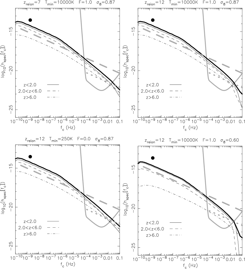
Figure 6: The characteristic strain spectrum. In each panel the thin lines in order from bottom to top show the spectrum in different redshift intervals and the thick dark solid line is the total strain spectrum. The thick dashed line shows the characteristic spectrum $h_{\rm spec}=10^{-21}f_{\rm c}^{-2/3}$ found by Jaffe & Backer (2002), and the thick dotted line the estimated stellar binary foreground from Phinney (2001). The thick grey solid line in the lower right corner of each panel shows the expected instrumental noise for LISA. The dot shows the current limit from pulsar timing. The panels show cases I-IV whose primary parameters are listed at the top of each plot. We assume $\epsilon_{0}=10^{-5.4}$ and $\gamma=5$.

At frequencies between $10^{-9}$Hz and $10^{-6}$Hz, the characteristic strain spectrum has a logarithmic slope of -2/3. This slope results from the dependence of energy loss on frequency as explained by Phinney (2001). At the higher frequencies relevant for LISA, we find departures from the -2/3 slope. The steepening of $h_{\rm spec}(f_{\rm c})$ is due to the loss of power at high frequencies associated with the maximum frequency during inspiral. At frequencies below $10^{-9}$Hz there is loss of power arising because many very low frequency sources do not coalesce within a Hubble time. The thick grey lines in the lower right corner of each panel in Figure 6 show the instrumental noise equivalent of $h_{\rm spec}$ computed from the instrumental noise spectral amplitude $S_{\rm h}^{\rm inst}(f_{\rm c})$. The curves are from a fit (Hughes 2002) to calculations of $S_{\rm h}^{\rm inst}(f_{\rm c})$ (Folkner 1998). The amplitude of the characteristic strain spectrum should be detectable by LISA over the frequency range $\sim 10^{-4}$–$10^{-2}$Hz. However the low numbers of events will make the power-spectrum noisy in this regime. In general the binaries can be resolved provided less than 20% of the frequency bins are filled at any one time. As we showed in § 5, most events are of sufficiently short duration to allow each to be resolved separately. The white-dwarf/white-dwarf binary foreground was estimated by Phinney (2001) and is plotted as the thick dotted lines [cut off below $10^{-4}$Hz since low frequency binaries are not expected to contribute significant gravitational waves (Hils, Bender, & Webbink 1991). Through most of the LISA band, this foreground is more than an order of magnitude below the expected background due to coalescing massive BH binaries.

We also show in Figure 6 the current upper limits on the GW background (large dots). The most recent limits are quoted by Lommen (2002). They find a limit on the fractional energy density in gravitational waves per logarithm of frequency at $f_{\rm c}=1.9\times 10^{-9}$Hz is $\Omega_{\rm g}h^{2}<2\times 10^{-9}$. We then find a corresponding limit on the characteristic strain spectrum of $h_{\rm spec}(1.9\times 10^{-9}$Hz$)<3\times 10^{-14}$. The limits are close to the theoretical spectrum in cases I-III. We will return to this important and unexpected result below.

Our results in cases I–III for the amplitude of the characteristic strain spectrum are different from the findings of Jaffe & Backer (2002) in the regime accessible to pulsar timing. In particular we find that the models predict $h_{\rm spec}(1.9\times 10^{-9}$Hz$)$ that is an order of magnitude higher than predicted by Jaffe & Backer (2002), and which is close to the limits of detection by the pulsar timing measurements. There are several possible causes for this difference. Jaffe & Backer (2002) use a power-law extrapolation of an estimate of the spheroid merger rate to higher redshifts, while in fact galaxies were made of smaller sub-units that had a higher merger probability at earlier cosmic times. Also, they use a phenomenological prescription for the merger rate that may substantially underestimate the actual merger rate for short duty cycle events. Furthermore, they assume the same merger rate for all galaxies, and do not assign a relation between black-hole and galaxy mass. In essence, we have assumed BHs to be associated with dark-matter halos, for which the merger history is understood rather than use an estimate of the average spheroid merger rate. The two assumptions lead to different results because the total merger rate of galaxies above the cooling threshhold as computed from the Press-Schechter formalism is higher than estimates of the observed spheroid merger rate. We find that if we artificially force equality between the merger rates computed in our work and those used in Jaffe & Backer (2002), we obtain a similar spectrum well below current limits.

The results should also be dependent on the BH – halo mass relation. The amplitude of $h_{\rm spec}$ is proportional to $\epsilon_{0}^{5/3}$ [see equation (8), (21) and (22)]. As a result, a lower value of $\epsilon_{0}$ will result in $h_{\rm spec}$ having a lower amplitude. Moreover, the production of power at very low frequencies is dominated by very large BHs, and so $h_{\rm spec}$ should be sensitive to $\gamma$, with larger $\gamma$ values resulting in larger amplitudes. We note that the log-normal distribution employed by Jaffe & Backer (2002) is steeper at the highest masses than our BH mass function computed from the Press-Schechter mass function and the $M_{\rm bh}-M$ relation, which might further contribute to our differing results. We will return to the dependence on the BH – halo mass relation in the following section (§ 6.2).

Our simulation of Case IV yields a value of $h_{\rm spec}(1.9\times 10^{-9}$Hz$)$ that is an order of magnitude below current limits, and which is more consistent with the findings of Jaffe & Backer (2002). Thus, the power in GWs is quite sensitive to the value of $\sigma_{8}$. Indeed $h_{\rm spec}$ is significantly more sensitive to $\sigma_{8}$ than to the details of the merger history provided that the history results in BHs being ubiquitous in massive galaxies in the local universe.

We find that the characteristic strain spectrum at low frequencies is dominated by galaxies having masses larger than $\sim 10^{12}M_{\odot}$ merging at redshifts below the peak in quasar activity ($z\lesssim 2$). This is particularly true of case IV. Theoretical studies of the quasar luminosity function find that the lack of cold gas at low redshifts explains the drop in quasar activity in massive galaxies (Kauffmann & Haehnelt 2000). If as suggested (e.g. Gould & Rix 2000) gas that is driven to the center of the galaxy during a merger is the mechanism that brings the BH binary into the GW dominated regime, then we might expect galaxy mergers to be inefficient ($\epsilon_{\rm mrg}\ll 1$) at producing gravitational radiation at low redshifts. If $\epsilon_{\rm mrg}\ll 1$, then we expect the amplitude of $h_{\rm spec}$ which is proportional to $\sqrt{\epsilon_{\rm mrg}}$, to be lower than predicted. Our results from cases I-III imply that limits on the efficiency can already be placed for some values of $\gamma$ and $\epsilon_{0}$ using limits on $h_{\rm spec}$ from pulsar timing experiments (§ 6.2). If $\epsilon_{\rm mrg}$ is found to have a value of order unity through the detection of the background by future pulsar timing experiments or by the LISA satellite, then this would strengthen the case for similar values at yet higher redshifts. The number counts of mergers detected by LISA will therefore directly determine the BH occupation fraction at high redshift.

6.2 Limits on $\epsilon_{0}$ and $\gamma$

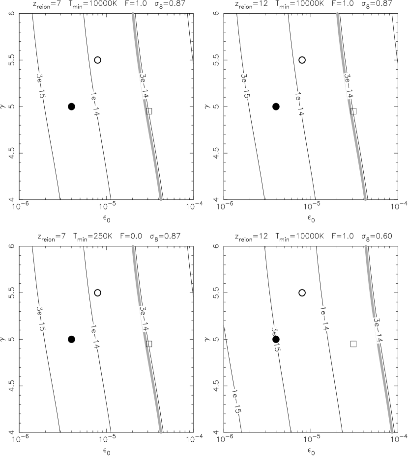
Figure 7: Contours of the value of the characteristic strain spectrum at $f_{\rm c}=1.9\times 10^{-9}$Hz as a function of $\epsilon_{0}$ and $\gamma$. The thick line shows the current upper limit from pulsar timing experiments. The dot shows the position of the parameter pair $\epsilon_{0}=10^{-5.4}$, $\gamma=5$. The open circle the values found by Ferrarese (2002) assuming that the circular velocity equals the virial velocity ($\gamma=5.46,\epsilon_{0}=10^{-5.06}$), while the square shows the observed values ($\gamma=4.95,\epsilon_{0}=10^{-4.54}$) assuming an NFW profile (Bullock et al. 2001). The panels show cases I-IV whose primary parameters are listed at the top of each plot.

The models considered in this paper predict characteristic strain spectra with values at $f_{\rm c}=1.9\times 10^{-9}$Hz that are close to the current limits from pulsar timing experiments (Kaspi et al. 1994; Thorsett & Dewey 1996 and Lommen 2002). So far we have concentrated on the spectrum and event rate for $\epsilon_{0}=10^{-5.4}$ and $\gamma=5$, which are the values favored by simple feedback arguments and the theoretical model for the quasar luminosity function described in Wyithe & Loeb (2002). However variation of $\epsilon_{0}$ and $\gamma$ has a significant effect on the GW signal. Since $h_{\rm spec}$ is dominated by the mergers of massive ($\gtrsim 10^{12}M_{\odot}$) galaxies at low redshifts ($z\lesssim 2$) in which supermassive BHs are thought to be ubiquitous, it should be quite insensitive to the details of the uncertain evolution in the BH mass function at higher redshifts. The amplitude of $h_{\rm spec}(1.9\times 10^{-9}{\rm Hz})$ therefore provides robust constraints on combinations of the parameters $\epsilon_{\rm mrg}$, $\gamma$ and $\epsilon_{0}$.

In Figure 7 we show contours of $h_{\rm spec}(1.9\times 10^{-9}{\rm Hz})$ as a function of $\epsilon_{0}$ and $\gamma$. The thick grey line shows the contour at the current limit of $h_{\rm spec}<3\times 10^{-14}$. The dot shows the values $\epsilon_{0}=10^{-5.4}$ and $\gamma=5$. As mentioned the value is close to the observational limits. The open circle shows the values found by Ferrarese (2002) assuming the circular velocity equals the virial velocity ($\gamma=5.46,\epsilon_{0}=10^{-5.06}$), which is the assumption implicit within our formalism. The square shows the corresponding observed values ($\gamma=4.95,\epsilon_{0}=10^{-4.54}$) obtained assuming a Navarro, Frenk & White (1997) profile (Bullock et al. 2001). We see that if coalescence is prompt for all binaries, then the pulsar measurements already exclude parameter space close to the currently favorable values.

Adoption of the values determined by Ferrarese (2002) for the BH – halo mass relation implies either that the background will soon be detected, or that the efficiency for BH binary coalescence at low redshift is $\epsilon_{\rm mrg}<1$. Yu (2002), investigated the evolution of hypothetical BH binaries in realistic models of nearby early-type galaxies. She found that BH binaries are likely to survive for longer than a Hubble time in spherical or weakly flattened/triaxial galaxies. No evidence has yet been found for BH binaries in the centers of the galaxies studied. The upper limit of the range of semimajor axes of surviving binary black holes as determined by Yu (2002) is close to the HST resolution for typical nearby galaxies (i.e., galaxies at Virgo). Thus, the absence of evidence for double nuclei in nearby galactic centers does not necessarily mean that they have no BH binaries (Q. Yu, private communication). Further improvement by an order of magnitude in the upper limits on the GW background will imply that $\epsilon_{\rm mrg}<1$ and that BH binaries may survive in galaxies rather than coalesce. Yu (2002) also computed the periods of surviving BH binaries. Of particular importance to this study is that nearly all of the surviving BH binaries would have periods longer than 20 yrs, and would therefore not contribute to $h_{\rm spec}(1.9\times 10^{-9}Hz)$.

7 Conclusions

We have computed the characteristic strain spectrum for GWs, as well as the number of events detectable by the planned LISA observatory due to coalescing massive BH binaries. Rather than adopt a phenomenological approach which is limited by the redshift horizon of current observations, we calculated the expected merger history of galaxies out to arbitrarily high redshifts under different assumptions. Our model uses the observed relation (Ferrarese 2002) between the circular velocity of galaxies and their central BH mass, and assumes that massive BHs form in galaxies into which gas can condense and cool. An important ingredient in the prescription is the observation that the slope and normalization of the relation holds out to high redshift (Shields et al. 2002). The underlying principles of this approach have been shown to reproduce current data on the luminosity function of quasars (Wyithe & Loeb 2002; Volonteri, Haardt & Madau 2002).

We find that if BH formation is ongoing in galaxies with masses above the cooling threshhold, then reionization produces a sharp drop in the number counts of LISA sources as a function of source redshift (see Fig. 3). In the instance that all binary BHs proceed to coalescence our models generically predict that hundreds of events with strains $h_{c}>10^{-22}$ will be detectable per year by LISA. The strongest sources have short durations and will not suffer from a confusion limit. Interestingly, most of these sources originate from redshifts $z>7$.

In the nHz regime accessible to pulsar timing experiments, we find that the amplitude of the characteristic strain spectrum (related to the power in the gravitational wave background) is close to current limits assuming values (favored by Wyithe & Loeb 2002) of $\gamma=5$ and $\epsilon_{0}=10^{-5.4}$ for the slope and normalization relating the BH to host galactic halo mass (see equation 4). Based on local observational data on early type galaxies, Ferrarese (2002) finds $\gamma=5.46$ and $\epsilon_{0}=10^{-5.06}$ (where the circular velocity is assumed to equal the virial velocity), or $\gamma=4.95$ and $\epsilon_{0}=10^{-4.54}$ (where the halo density is assumed to follow an NFW profile). Calculations of the characteristic strain spectrum assuming these parameter sets are comparable to current limits, and already rule out only slightly different combinations of $\gamma$ and $\epsilon_{0}$ if all binary black holes proceed to coalescence. Alternatively, future improvements in the observational limits will allow limits to be placed on the fraction of black hole binaries that proceed to coalescence from calculations of the strain spectrum that use measured values of $\gamma$ and $\epsilon_{0}$.

We find that the amplitude of the characteristic spectrum of strain is dominated by the mergers of massive galaxies ($M\gtrsim 10^{12}M_{\odot}$) at low redshift ($z\lesssim 2$). As a result, $h_{\rm spec}$ is quite sensitive to the value of $\sigma_{8}$. Since BHs are ubiquitous in the local universe, detection of the background either by future pulsar timing measurements or by the LISA satellite will determine the efficiency with which binary BHs coalesce.

Observations of GWs are likely to provide insight into the formation history of massive BHs. LISA will open a new window to studies of the high redshift universe. The number counts of gravitational wave sources will provide an unprecedented probe of the reionization epoch, and constrain the merger rate of galaxies and the growth history of black holes at early epochs that are not yet probed by conventional astronomical telescopes. Pulsar timing arrays are suitable to measure the background arising from BH binaries at lower redshifts.

References

- (1) Abel, T., Bryan, G.L. & Norman, M.L., 2000, ApJ, 540, 39
- Armitage & Natarajan (2002) Armitage, P. J. & Natarajan, P. 2002, ApJ, 567, L9
- (3) Bardeen, J.M., Bond, J.R., Kaiser, N., & Szalay, A.S. 1986, ApJ, 304, 15
- Barkana & Loeb (2000) Barkana, R. & Loeb, A. 2000, ApJ, 539, 20
- (5) Barkana, R., & Loeb, A. 2001, Phys. Rep., 349, 125
- (6) Barkana, R., & Loeb, A. 2002, astro-ph/0209515
- Begelman, Blandford, & Rees (1980) Begelman, M. C., Blandford, R. D., & Rees, M. J. 1980, Nature, 287, 307
- (8) Bond, J.R., Cole, S., Efstathiou, G., & Kaiser, N. 1991, ApJ, 379, 440
- Bullock et al. (2001) Bullock, J. S., Kolatt, T. S., Sigad, Y., Somerville, R. S., Kravtsov, A. V., Klypin, A. A., Primack, J. R., & Dekel, A. 2001, MNRAS, 321, 559
- Colpi, Mayer, & Governato (1999) Colpi, M., Mayer, L., & Governato, F. 1999, ApJ, 525, 720
- (11) Fan, X., et al. 2001 AJ, 122, 2833
- (12) Ferrarese, L. 2002, ApJ, 578, 90
- Ferrarese et al. (2001) Ferrarese, L., Pogge, R. W., Peterson, B. M., Merritt, D., Wandel, A., & Joseph, C. L. 2001, ApJ, 555, L79
- (14) Folkner, W.M., 1998, in Folkner W.M., ed., AIP Conf. Proc. Vol. 456, Laser Interferometer Space Antenna, 2nd Int. LISA Symp. on the Detection and Observation of Gravitational Waves in Space. AIP, New York, p. 11
- Fukushige, Ebisuzaki, & Makino (1992) Fukushige, T., Ebisuzaki, T., & Makino, J. 1992, ApJ, 396, L61
- Ghigna et al. (1998) Ghigna, S., Moore, B., Governato, F., Lake, G., Quinn, T., & Stadel, J. 1998, MNRAS, 300, 146
- Gould & Rix (2000) Gould, A. & Rix, H. 2000, ApJ, 532, L29
- Haehnelt (1994) Haehnelt, M. G. 1994, MNRAS, 269, 199
- Haehnelt (1998) Haehnelt, M. G. 1998, AIP Conf. Proc. 456: Laser Interferometer Space Antenna, Second International LISA Symposium on the Detection and Observation of Gravitational Waves in Space, 45
- Haehnelt & Kauffmann (2002) Haehnelt, M. G. & Kauffmann, G. 2002, MNRAS, 336, L61
- Haehnelt, Natarajan, & Rees (1998) Haehnelt, M. G., Natarajan, P., & Rees, M. J. 1998, MNRAS, 300, 817
- Haiman, Abel, & Rees (2000) Haiman, Z. ;., Abel, T., & Rees, M. J. 2000, ApJ, 534, 11
- Hils, Bender, & Webbink (1991) Hils, D., Bender, P. L., & Webbink, R. F. 1991, ApJ, 369, 271
- Hughes (2001) Hughes, S. A., Marka, S., Bender, P.L., & Hogan, C.J., 2001, astro-ph/0110349
- Hughes (2002) Hughes, S. A., Blandford, R.D., 2002, astro-ph/0208484
- Hughes (2002) Hughes, S. A. 2002, MNRAS, 331, 805
- (27) Jaffe, A.H., Backer, D.C., 2002, astro-ph/0210148
- (28) Jenkins, A. et al. 2001, MNRAS, 321, 372
- Kaspi, Taylor, & Ryba (1994) Kaspi, V. M., Taylor, J. H., & Ryba, M. F. 1994, ApJ, 428, 713
- Kauffmann & Haehnelt (2000) Kauffmann, G. & Haehnelt, M. 2000, MNRAS, 311, 576
- Kitayama & Ikeuchi (2000) Kitayama, T. & Ikeuchi, S. 2000, ApJ, 529, 615
- Laor (2001) Laor, A. 2001, ApJ, 553, 677
- Lacey & Cole (1993) Lacey, C. & Cole, S. 1993, MNRAS, 262, 627
- (34) Lommen, A. N. 2002, astro-ph/0208572
- Magorrian et al. (1998) Magorrian, J. et al. 1998, AJ, 115, 2285
- Merritt & Ferrarese (2001) Merritt, D. & Ferrarese, L. 2001, ApJ, 547, 140
- Menou, Haiman, & Narayanan (2001) Menou, K., Haiman, Z. ;., & Narayanan, V. K. 2001, ApJ, 558, 535
- Milosavljević & Merritt (2001) Milosavljević, M. ; & Merritt, D. 2001, ApJ, 563, 34
- Navarro, Frenk, & White (1997) Navarro, J. F., Frenk, C. S., & White, S. D. M. 1997, ApJ, 490, 493
- Navarro & Steinmetz (1997) Navarro, J. F. & Steinmetz, M. 1997, ApJ, 478, 13
- (41) Peters, P.C., 1964, Phys Rev 136, B1224
- (42) Phinney, S., 2001, astro-ph/0108028
- (43) Press, W. H., & Schechter, P. 1974, ApJ, 187, 425
- Quinn, Katz, & Efstathiou (1996) Quinn, T., Katz, N., & Efstathiou, G. 1996, MNRAS, 278, L49
- Rajagopal & Romani (1995) Rajagopal, M. & Romani, R. W. 1995, ApJ, 446, 543
- (46) Seto, N., 2002, gr-qc/0210028
- (47) Shapiro, S.L. & Teukolsky, S.A., 1983, Black Holes, White Dwarfs, and Neutron Stars (new York : Wiley-Interscience)
- Sheth & Tormen (1999) Sheth, R. K. & Tormen, G. 1999, MNRAS, 308, 119
- (49) Shields, G.A., Gebhardt, K., Salviander, S., Wills, B., Xie, B., Brotherton, M., Yuan, J., Dietrich, M., 2002, astro-ph/0210050
- Silk & Rees (1998) Silk, J. & Rees, M. J. 1998, A&A, 331, L1
- (51) Thorne, K.S., 1987, in Hawking, S. & Israel, W., eds, 300 Years of Gravitation. Cambridge Univ. Press, Cambridge, p. 330
- Thorsett & Dewey (1996) Thorsett, S. E. & Dewey, R. J. 1996, Phys. Rev. D, 53, 3468
- (53) Thoul, A.A. & Weinberg, D.H., 1996, ApJ, 465, 608
- Tremaine et al. (2002) Tremaine, S. et al. 2002, ApJ, 574, 740
- (55) Volonteri, M., Haardt, F., Madau, P., 2002, astro-ph/0207276
- Weinberg, Hernquist, & Katz (1997) Weinberg, D. H., Hernquist, L., & Katz, N. 1997, ApJ, 477, 8
- (57) Wyithe, J.S.B, Loeb, A., 2002, astro-ph/0206154
- Yu (2002) Yu, Q. 2002, MNRAS, 331, 935