X-ray Emission Line Profile Modeling of O Stars:
Fitting a Spherically-Symmetric Analytic Wind-Shock Model to the Chandra Spectrum of $\zeta$ Puppis

Abstract

X-ray emission line profiles provide the most direct insight into the dynamics and spatial distribution of the hot, X-ray-emitting plasma above the surfaces of OB stars. The O supergiant $\zeta$ Puppis shows broad, blueshifted, and asymmetric line profiles, generally consistent with the wind-shock picture of OB star X-ray production. We model the profiles of eight lines in the Chandra HETGS spectrum of this prototypical hot star. The fitted lines indicate that the plasma is distributed throughout the wind starting close to the photosphere, that there is significantly less attenuation of the X-rays by the overlying wind than is generally supposed, and that there is not a strong trend in wind absorption with wavelength.

1 Introduction

The nature of the copious soft X-ray emission from hot stars has been a longstanding controversy since its discovery in the late 1970s (Harnden et al., 1979; Cassinelli & Olson, 1979). Solar-type coronal emission was first assumed (Cassinelli & Olson, 1979; Waldron, 1984), but wind-shock models of various types gained currency throughout the following decade (Waldron, 1984; Owocki, Castor, & Rybicki, 1988; MacFarlane & Cassinelli, 1989; Chen & White, 1991; Hillier et al., 1993; Cohen et al., 1996; Feldmeier et al., 1997; Feldmeier, Puls, & Pauldrach, 1997). More recently, hybrid magnetic wind models have been proposed for some hot stars (Gagné et al., 1997; Babel & Montmerle, 1997; ud-Doula & Owocki, 2002).

Until the launch of Chandra and XMM, no observational diagnostics were available that could provide a direct discriminant between the coronal and wind-shock paradigms. But due to their superior spectral resolution, both of these new telescopes allow for the separation of individual emission lines and the resolution of Doppler-broadened line profiles. The spectral resolution of Chandra’s grating spectrometers exceeds $\frac{\lambda}{\Delta\lambda}\sim 1000$ (for the FWHM) which corresponds to a velocity of $300$ km s^-1, and that of the XMM RGS is almost as great. This compares favorably to the terminal velocities of the radiation-driven winds of O stars, which approach $v_{\infty}=3000$ km s^-1, implying $\sim 20$ resolution elements for a velocity range of $2v_{\infty}$.

At the most basic level, the X-ray emission lines from hot stars will either be narrow and therefore roughly consistent with coronal emission or broad and roughly consistent with wind-shock emission. This is because in the wind-shock model the high velocities of X-ray-emitting plasma embedded in the wind would Doppler-shift the emission across a range of wavelengths. Initial papers reporting on Chandra and XMM observations of various O and B stars (Schulz et al., 2001; Kahn et al., 2001; Waldron & Cassinelli, 2001; Cassinelli et al., 2001; Miller et al., 2002; Cohen et al., 2003) discussed line widths, which vary from large for early O stars to small for B stars. Some of these initial studies noted that the emission lines can be blueshifted and the profiles somewhat asymmetric, but none of these studies discussed or modeled the shapes of the resolved emission lines.

In this paper we fit a specific model of X-ray emission line profiles in an expanding, emitting, and absorbing wind to a Chandra HETGS/MEG spectrum of $\zeta$ Puppis. The model we fit is empirical and flexible, with only three free parameters. The model assumes a two-component fluid, having as its major constituent the cold, X-ray-absorbing plasma that gives rise to the characteristic UV absorption lines observed in hot star winds, and as its minor constituent the hot, X-ray-emitting plasma. This empirical model is not tied to any one specific physical model of X-ray production, and is general enough to fit data representative of any of the major models, so long as they are spherically symmetric. To the extent that wind-shock models are found to be consistent with the observed line profiles, our model parameters can be used to constrain the physical properties of the shock-heated plasma. This ultimately can be used to constrain the values of the physical parameters of the appropriate wind-shock model.

In section 2 we discuss the physical effects leading to non-trivial line shapes and describe the specific empirical model we use to perform the fits. In section 3 we describe the Chandra $\zeta$ Puppis dataset and how we perform the line fitting and parameter estimation. And in section 4 we discuss the derived model parameters in the context of the various physical models that have been proposed to explain hot-star X-ray emission, as well as in the context of other X-ray diagnostics that have recently been applied to the data from this star.

2 Theoretical Considerations

In the context of the fast, radiation-driven winds of OB stars, a source of X-ray emission embedded in the wind will lead to Doppler broadened profiles, but only the X-ray emitting plasma traveling at the wind terminal velocity directly toward or away from the observer will lead to maximal blueshifts and redshifts. The amount of emission at each intermediate wavelength, and thus the shape and characteristic width of the line, depends on the spatial and velocity distribution of the hot plasma. As described by MacFarlane et al. (1991) in the case of a shell of X-ray emitting plasma in a hot star wind, the continuum absorption of X-rays by the cool component of the wind will cause the resulting emission lines to be attenuated on the red side and be relatively unaffected on the blue side of the line profile. The apparent peak of the emission line thus shifts to the blue side of line center, and the line is asymmetric, with a shallower red wing and a steeper blue wing.

This basic idea of Doppler broadened emission from a hot wind component and continuum absorption by the cool wind component leading to a broadened, shifted, and asymmetric line was extended from a shell to a spherically symmetric wind by Ignace (2001). He showed that model line profiles could be generated analytically for a constant-velocity wind. Owocki & Cohen (2001) extended this concept further, to an accelerating wind, with a model having four free parameters. Two describe the spatial distribution of the X-ray emitting plasma – $R_{\mathrm{o}}$, the minimum radius of X-ray emission and $q$, the radial power-law index of the emissivity. There is assumed to be no emission below $r=R_{\mathrm{o}}$. Above $r=R_{\mathrm{o}}$, volume emissivity is assumed to scale like the density of the wind squared $\rho^{2}$ (since collisional processes and recombination dominate the ionization/excitation kinematics), with an extra factor $r^{-q}$ allowing for spatial variation of shock temperatures, cooling structures, and density and filling factor of the shocked material. The parameter $\beta$ controls the velocity of the wind, which is assumed to follow a “beta-velocity law”:

$$v(r)=v_{\infty}(1-R_{*}/r)^{\beta}\;\mathrm{.}$$ (1)

Both components of the wind follow the same velocity law in all cases discussed here, but in principle they could be allowed to differ. The fourth parameter, $\tau_{*}$, characterizes the amount of absorption in the wind

$$\tau_{*}\equiv\frac{\kappa\dot{M}}{4\pi v_{\infty}R_{*}}\text{ ,}$$ (2)

where $\kappa$ is the line opacity or mass absorption coefficient (cm² s^-1). This relates to the commonly-quoted radius of optical depth unity $R_{1}$ by the equation (for $\beta=1$)

$$\frac{R_{1}}{R_{*}}=\frac{1}{1-\exp{(-1/\tau_{*})}}\approx\tau_{*}+0.5\text{ for $\tau_{*}>0.5$.}$$ (3)

The error in the above approximation is less than 10% for $\tau_{*}>0.67$ (or $R_{1}/R_{*}>1.3$).

The model put forward by Owocki & Cohen (2001) is a phenomenological one. It describes the physical properties of the hot and cool components of the wind, but does not describe the physics underlying the generation of the hot plasma. It is therefore quite flexible, capable of describing a thin shell of X-ray emitting plasma, including a coronal-type zone near the photosphere, as well as wind shocks distributed spatially throughout the wind, with the shock distribution and wind velocity varying with radius. This model is thus capable of constraining properties of both the X-ray-emitting and the X-ray-absorbing wind components. When applied to an ensemble of lines it has the potential to constrain these properties as a function of both temperature and wavelength. Assuming turbulent and thermal broadening are negligible and combining the other model assumptions, the line profile as a function of scaled wavelength $x\equiv(\lambda/\lambda_{0}-1)(c/v_{\infty})$ is given by

$$L_{\mathrm{x}}\propto\int_{r=r_{x}}^{\infty}\frac{r^{-(q+2)}}{\left(1-\frac{R_{*}}{r}\right)^{3\beta}}\exp\left[-\tau\left(\mu_{x},\;r\right)\right]dr\text{ ,}$$ (4)

where $r_{x}\equiv\max\left[R_{\mathrm{o}},R_{*}/(1-|x|^{(1/\beta)})\right]$, $\mu_{x}\equiv x/(1-R_{*}/r)^{\beta}$ and $\tau\left(\mu,r\right)$ (which is proportional to $\tau_{*}$) is the optical depth along the observer’s line of sight at direction cosine $\mu$ and radial coordinate $r$. The constant of proportionality (which is, itself, proportional to the emission measure) will not be determined in this work. Equation (4) must be solved numerically, except in the case of $\beta=0$ (constant velocity wind). And even so, we only obtain solutions for integer values of $\beta$.

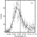
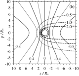
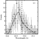
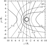
Figure 1: Two representative lines with best-fit models. Shown are Chandra MEG spectra of (a) Fe XVII at 15.01 Å and (c) O VIII at 18.97 Å (in gray), with corresponding best-fit profiles (in black). Laboratory rest wavelengths are indicated by the vertical dashed lines. To the right we show (b and d) contour plots representing the models. The observer is located at $(p/R_{*}=0,z/R_{*}=\infty)$. The inner circle is of radius $R_{*}$, the outer circle of radius $R_{\mathrm{o}}$. Gray contours are curves of constant line-of-sight velocity component in units of $v_{\infty}$. Dashed contours are curves of constant optical depth ($\tau=0.5,1,2$), integrated along the line of sight.

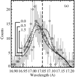
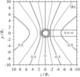
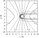
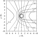
Figure 2: Models at extremes of the confidence region. Shown are the Chandra MEG spectrum of the 17.054 Å line of Fe XVII (in gray), and (in black) the best-fit model ($\tau_{*}=0.5$), the fit with $\tau_{*}$ held at its 95.4% confidence upper limit ($\tau_{*}=1.5$) and the fit with $\tau_{*}$ held at its 95.4% confidence lower limit ($\tau_{*}=0.0$). The contour plots are the same style as in Figure 1 and correspond to (b) the $\tau_{*}=0.0$ model, (c) the best-fit model, and (d) the $\tau_{*}=1.5$ model.

This model assumes implicitly that the sites of X-ray emission are so numerous and well-mixed with the primary cool wind component that we can treat the wind as a two-component fluid. It also neglects non-radial velocity components, including small scale fluctuations like turbulence. Note that the assumption of purely radial velocities is what allows wind absorption to break the symmetry of the line, since redshifted emission always arises at higher line-of-sight distances (and therefore higher optical depths) than the blueshifted emission (see the contour plots in Figures 1 and 2).

Similar treatments of radiation transport have previously been fitted to the global form of low-resolution spectra (Hillier et al., 1993; Feldmeier et al., 1997). MacFarlane et al. (1991) and Waldron & Cassinelli (2001) have modeled line profiles from discrete spherical shocks. Elsewhere we report on the investigation of non-spherical models and their applicability to hot stars (Kramer et al., 2003; Tonnesen et al., 2003).

For this study, we have adopted the Owocki & Cohen (2001) model and performed fits on eight strong lines in the Chandra HETGS spectrum of the O4 supergiant $\zeta$ Puppis, extracting best-fit values and associated confidence limits for three model parameters: $q$, $R_{\mathrm{o}}$, and $\tau_{*}$.

3 Fitting the Model to Observed Line Profiles

Our data set consists of the $\pm 1$ order MEG spectrum from a $67$ ks observation of the O4f star $\zeta$ Puppis first reported on by Cassinelli et al. (2001). The FWHM of the MEG spectral response is $\Delta\lambda_{\mathrm{MEG}}=0.023$ Å (Chandra X-Ray Center, 2001). All the distinguishable lines in this spectrum are many times more broad, allowing their profiles to be well resolved. The breadth of the lines means that many of them are contaminated by emission from neighboring lines. After eliminating He-like fir triplets as unsuitable for fitting due to excessive blending, we identified other potential blends by visual inspection of the spectrum and by referring to the line strengths calculated by Mewe, Gronenschild, & van den Oord (1985, Table IV) and those in the Astrophysical Plasma Emission Database (APED,  Smith et al., 2001). We consider a line with rest wavelength $\lambda_{0}$ to extend over a wavelength range defined by

$$\lambda_{0}\left(1+\frac{v_{\infty}}{c}\right)+\Delta\lambda_{\mathrm{MEG}}\geq\lambda\geq\lambda_{0}\left(1-\frac{v_{\infty}}{c}\right)-\Delta\lambda_{\mathrm{MEG}}\;\mathrm{.}$$ (5)

The widths of neighboring lines are calculated the same way, and any overlap in the ranges is excluded from the fit (see Table 1 for the wavelength range over which each fit was performed). We adopted the terminal velocity value determined by Prinja, Barlow, & Howarth (1990), $v_{\infty}=2485\;\mathrm{km\ s}^{-1}$.

We numerically integrate equation (4) over the desired wavelength range using software written in Mathematica. The resulting profile is convolved with a Gaussian representing instrumental response, binned identically to the data, and normalized to predict the same total number of counts as were observed over the same wavelength range.

To properly treat the statistics of Poisson-distributed, low-photon-count data, we use Cash’s $C$ (Cash, 1979) as the fit statistic. Fits are performed by calculating $C$ on a grid in parameter space. The coordinates of the parameter-space point producing the minimum $C$ value $C_{\mathrm{min}}$ are taken as our “best-fit” parameters. We then use limits on $\Delta C=C-C_{\mathrm{min}}$ to define our confidence regions, as described by Cash (1979). The grid is expanded as needed until the entire confidence region is encompassed within it. In all our fits we held $\beta$ constant at $\beta=1$ (which is very close to the typical O-star value of 0.8, Groenewegen et al., 1989) and varied $R_{\mathrm{o}}$, $q$, and $\tau_{*}$.

To confirm the confidence limits derived using the $\Delta C$ statistic, we carried out the fitting procedure on monte carlo simulated data sets and compared the parameter-space distribution of simulated-data fit parameters to the calculated $\Delta C$ confidence region for each line. The monte carlo simulations gave results that were consistent with those given by the $\Delta C$ statistic.

The quality of the fits was evaluated using the Kuiper statistic, a variant of the Kolmogorov-Smirnov test. Significance levels were determined using monte carlo techniques. We obtained two slightly different distributions of the Kuiper statistic depending on whether the simulated data sets were compared directly to the parent model (giving significance level $\alpha_{0}$) or compared to a new best-fit model found by performing the fitting procedure on the simulated data set (giving significance level $\alpha_{\mathrm{RF}}$).

In all, we fit eight lines between 6.18 Å (Si XIV) and 24.78 Å (N VII). The results are listed in Table 1, and shown in Figure 1 for two representative lines. All the fits but one are formally good according to both distributions. The value of $\alpha_{0}=0.039$ for the 15.262 Å fit does not meet the criterion $\alpha\geq 0.05$ for a formally-good fit. This line may be contaminated by the Fe XIX lines at 15.198 Å and 15.3654 Å (APED). The relatively-low significance values for the N VII line may simply be the result of random variation, or could be a sign that there are resolved spectral features not explained by this simple model. In any case, the fit is formally good. The 16.787 Å fit may also be affected by a blend with an Fe XIX line, this one at 16.718 Å. This would add flux to the blue edge of the line, increasing its skew and explaining the relatively high values of $\tau_{*}$ and $q$.

To demonstrate the typical range of models that can be fit to one line, we show the best-fit and two extreme models superimposed on the Fe XVII line at 17.05 Å in Figure 2. The two extreme models are for the parameter sets that have the largest and smallest values of $\tau_{*}$ within the 95.4% confidence region.

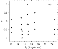
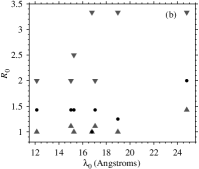
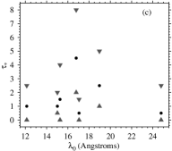
Figure 3: The best-fit values of (a) $q$, (b) $R_{o}$ in units of $R_{*}$, and (c) $\tau_{*}$ for seven of the eight lines (bullets), along with the range given by the 95.4% confidence limits (triangles). See Table 1.

Finally, we summarize the best-fit and 95.4% confidence limits of the three free model parameters for seven of the eight lines in Figure 3 (the values for the Si XIV line are not shown because it is at a much shorter wavelength and its fit parameters are poorly constrained). Trends in these fitted parameters and their implications are discussed in the next section.

4 Discussion

The primary result of the analysis presented in this paper is that the X-ray emission lines in the prototypical O supergiant, $\zeta$ Puppis, can, for the most part, be adequately fit with a spherically symmetric wind model having a small number of free parameters. Furthermore, the derived parameters are quite reasonable in the context of most wind-shock models, being consistent with hot plasma uniformly distributed throughout the wind above a moderate onset radius, X-ray emitting plasma extending out to the wind terminal velocity, and the need for the inclusion of some wind attenuation.

In detail, however, some interesting trends emerge. First of all, the amount of wind attenuation is significantly smaller than what one might expect from a spherically symmetric smooth wind, given what is known about this star’s mass-loss rate and wind opacity. There have been various calculations of the wind optical depth (often expressed as the radius of optical depth unity) as a function of wavelength for this star. They range from values much bigger than what we derive here ($7<\tau_{*}<30$ calculated by Hillier et al., 1993, using $\dot{M}=5.0\times 10^{-6}~{}\mathrm{M}_{\sun}~{}\mathrm{yr}^{-1}$, $R_{*}=19~{}R_{\sun}$, $v_{\infty}=2200$ km s^-1), to values modestly bigger ($4<\tau_{*}<8$ calculated by Cassinelli et al., 2001, using values from Lamers & Leitherer, 1993: $\dot{M}=2.4\times 10^{-6}~{}\mathrm{M}_{\sun}~{}\mathrm{yr}^{-1}$, $R_{*}=16~{}R_{\sun}$, $v_{\infty}=2200$ km s^-1). Note that Hillier et al. (1993) find different values for $R_{1}$ depending on whether helium recombines or remains ionized in the outer wind, but at energies above 0.5 keV (where all of the lines presented here occur) there is little difference between the two scenarios. More recent stellar parameters determined by (Puls et al., 1996) ($\dot{M}=5.9\times 10^{-6}~{}\mathrm{M}_{\sun}~{}\mathrm{yr}^{-1}$, $R_{*}=19~{}R_{\sun}$, and $v_{\infty}=2250$ km s^-1) agree well with the values used by Hillier et al. (1993), but would increase the Cassinelli et al. (2001) $\tau_{*}$ values by a factor of 2, given the same opacity (see eq. 2).

If we accept the $\tau_{*}$ values derived from our fits, then the disparity between those values and the ones mentioned above suggest that either the mass-loss rates or wind opacities are being overestimated in previous calculations. The mass-loss rate of $\zeta$ Puppis is by now quite well established using UV absorption lines and H$\alpha$, although improper ionization corrections or clumping could lead to systematic errors. The wind opacity determination seems much more uncertain, both because of the inconsistent values in the literature and because of the difficulty in determining the ionization state of the wind (MacFarlane et al., 1993; MacFarlane, Cohen, & Wang, 1994). Recent advances in stellar atmosphere modeling may help to improve these determinations (Pauldrach, Hoffmann, & Lennon, 2001). Another means of lowering the wind attenuation is to clump the wind into small clouds that are individually optically thick rendering the wind porous and enhancing the escape probability of X-ray photons, thus lowering the mean wind opacity. This would also affect the mass-loss rate diagnostics, but is, itself, an independent effect.

An even more curious result of the $\tau_{*}$ fits is that they are nearly independent of wavelength. This is surprising because photoionization cross sections should scale roughly as a power of wavelength between $\lambda^{2}$ and $\lambda^{3}$ (Hillier et al., 1993). It is possible that the distribution of ionization edges could conspire to make this relationship much flatter over a small range of wavelengths (as the calculations from Cassinelli et al. (2001) seem to indicate). But wind clumping might play some role, here too. If the wind opacity is dominated by clumps that are individually optically thick across the wavelength range, then the opacity ceases to be a function of wavelength and instead depends on the physical cross sections of the clumps themselves. We note that the UV line opacity necessary to explain the observed absorption line profiles could, in principle, still be provided by the tenuous inter-clump wind, as the line cross sections are much bigger than the X-ray photoionization cross sections.

If $R_{1}\gg R_{\mathrm{o}}$, the line profile is insensitive to changes in $R_{\mathrm{o}}$, since emission much below $R_{1}$ is largely absorbed by the wind. The values we find for $R_{\mathrm{o}}$, though generally small, are comparable to our values of $R_{1}$ (from $\tau_{*}$ by eq. 3). It is hard to assess these relatively small onset radii in the context of the small (sometimes surprisingly small) values claimed on the basis of observed $f/i$ ratios in He-like ions (Cassinelli et al., 2001; Kahn et al., 2001; Waldron & Cassinelli, 2001). This is partially because we do not fit the profiles of any He-like lines (they are too blended) and partly because the most extreme results (smallest value for $R_{1}$) are for S XV, which is a higher ionization stage than any of the lines we fit.

The fit results for the parameter $q$ indicate that there is not a strong radial trend in the filling factor. One might expect some competition in a wind shock model between the tendency to have more and stronger shocks near the star, where the wind is still accelerating, and the tendency for shock heated gas to cool less efficiently in the far wind, where densities are low. Perhaps these two effects cancel to give the observed $q\approx 0$ relationship.

In conclusion, the simple, spherically symmetric wind shock model is remarkably consistent with the observed line profiles in $\zeta$ Puppis, providing the most direct evidence yet that some type of wind-shock model applies to this hot star. However, there are indications that the absorption properties of the wind of $\zeta$ Puppis, and perhaps other hot stars, must be reconsidered. We will fit this same model to the Chandra spectra of other hot stars in the future. But the lack of strong line asymmetries in stars such as $\zeta$ Ori and $\delta$ Ori and the narrow lines in $\theta^{1}$ Ori C and $\tau$ Sco indicate that spherically symmetric wind-shock models with absorption may not fit the data from these stars as well as they do $\zeta$ Puppis.

Table 1: Best-Fit Parameters with 95.4% Confidence Limits

Ion	$\lambda_{0}$ (Å)	$\lambda_{0}/\Delta\lambda$	$2v_{\infty}/\Delta v$	$q$	$R_{\mathrm{o}}$	$\tau_{*}$	$x_{\mathrm{min}}$	$x_{\mathrm{max}}$	$N_{\mathrm{obs}}$	$\alpha_{0}$	$\alpha_{\mathrm{RF}}$
N VII	$24.78$	$1077$	$18$	$-0.5_{-0.3}^{+0.6}$	$2._{-0.6}^{+1.3}$	$0.5_{-0.5}^{+2.}$	$-1.11$	$1.11$	$92$	$0.667$	$0.356$
O VIII	$18.97$	$825$	$14$	$-0.1_{-0.4}^{+0.6}$	$1.2_{-0.2}^{+2.1}$	$2.5_{-1.5}^{+2.5}$	$-1.04$	$1.14$	$69$	$0.941$	$0.790$
Fe XVII	$17.054$	$741$	$12$	$-0.6_{-0.2}^{+0.4}$	$1.4_{-0.3}^{+0.6}$	$0.5_{-0.5}^{+1.}$	$-0.74$	$1.16$	$54$	$0.971$	$0.950$
Fe XVII	$16.787$	$730$	$12$	$0.4_{-0.6}^{+0.6}$	$1.0_{-0}^{+2.3}$	$4.5_{-2.5}^{+3.5}$	$-1.16$	$0.74$	$53$	$0.517$	$0.490$
Fe XVII	$15.262$	$664$	$11$	$-0.8_{-0.2}^{+0.2}$	$1.4_{-0.4}^{+1.1}$	$1.5_{-1.5}^{+2.5}$	$-0.81$	$1.19$	$50$	$0.039$	$0.151$
Fe XVII	$15.013$	$653$	$11$	$-0.2_{-0.3}^{+0.4}$	$1.4_{-0.3}^{+0.6}$	$1.0_{-0.5}^{+1.}$	$-1.19$	$0.79$	$49$	$0.887$	$0.800$
Ne X	$12.13$	$527$	$9$	$-0.4_{-0.3}^{+0.5}$	$1.4_{-0.4}^{+0.6}$	$1.0_{-1.}^{+1.5}$	$-1.23$	$0.03$	$26$	$0.432$	$0.100$
Si XIV	$6.18$	$269$	$4$	$-0.2_{-0.8}^{+\;\cdots}$	$1.4_{-1.4}^{+8.6}$	$1.5_{-1.5}^{+5.5}$	$-0.98$	$0.59$	$16$	$0.857$	$0.622$

Note. — The width of the instrumental response in wavelength units is $\Delta\lambda=\Delta\lambda_{\mathrm{MEG}}=0.023$ Å, or in velocity units $\Delta v=c\Delta\lambda/\lambda_{0}$. The scaled wavelength $x\equiv(c/v_{\infty})(\lambda-\lambda_{0})/\lambda_{0}$. $N_{\mathrm{obs}}$ is the number of wavelength bins included in the fit.

References

- Babel & Montmerle (1997) Babel, J., & Montmerle, T. 1997, ApJ, 485, L29
- Cash (1979) Cash, W. 1979, ApJ, 228, 939
- Cassinelli et al. (2001) Cassinelli, J. P., Miller, N. A., Waldron, W. L., MacFarlane, J. J., & Cohen, D. H. 2001, ApJ, 554, L55
- Cassinelli & Olson (1979) Cassinelli, J. P., & Olson, G. L. 1979, ApJ, 229, 304
- Chandra X-Ray Center (2001) Chandra X-Ray Center. 2001, The Chandra Proposers’ Observatory Guide, v4.0, (Cambridge: Chandra X-Ray Center)
- Chen & White (1991) Chen, W., & White, R. L. 1991, ApJ, 366, 512
- Cohen et al. (1996) Cohen, D. H., Cooper, R. G., MacFarlane, J. J, Owocki, S. P., Cassinelli, J. P., & Wang, P. 1996, ApJ, 460, 506
- Cohen et al. (2003) Cohen, D. H., De Mèssieres, G. E., MacFarlane, J. J, Miller, N. A., Cassinelli, J. P., Owocki, S. P., & Liedahl, D. A. 2003, ApJ, in press
- Feldmeier et al. (1997) Feldmeier, A., Kudritzki, R.-P., Palsa, R., Pauldrach, A. W. A., Puls, J. 1997, A&A, 320, 899
- Feldmeier, Puls, & Pauldrach (1997) Feldmeier, A., Puls, J., & Pauldrach, A. W. A. 1997, A&A, 322, 878
- Gagné et al. (1997) Gagné, M., Caillault, J.-P., Stauffer, J. R., & Linsky, J. L. 1997, ApJ, 478, L87
- Groenewegen et al. (1989) Groenewegen, M. A. T., Lamers, H. J. G. L. M., & Pauldrach, A. W. A. 1989, A&A, 221, 78
- Harnden et al. (1979) Harnden, F. R., Jr. et al. 1979, ApJ, 234, L51
- Hillier et al. (1993) Hillier, D. J., Kudritzki R. P., Pauldrach, A. W., Baade, D., Cassinelli, J. P., Puls, J., & Schmitt, J. H. M. M. 1993, A&A, 276, 117
- Ignace (2001) Ignace, R. 2001, ApJ, 549, L119
- Kahn et al. (2001) Kahn, S. M., Leutenegger, M. A., Cotam, J., Rauw, G., Vreux, J.-M., den Boggende, A. J. F., Mewe, R., & Güdel, M. 2001, A&A, 365, L312
- Kramer et al. (2003) Kramer, R. H., Tonnesen, S. K., Cohen, D. H., Owocki, S. P., ud-Doula, A., & MacFarlane, J. J. 2003, Rev. Sci. Inst., in press
- Lamers & Leitherer (1993) Lamers, H. J. G. L. M., & Leitherer, C. 1993, ApJ, 412, 771
- MacFarlane & Cassinelli (1989) MacFarlane, J. J., & Cassinelli, J. P. 1989, ApJ, 347, 1090
- MacFarlane et al. (1991) MacFarlane, J. J., Cassinelli, J. P., Welsh, B. Y., Vedder, P. W., Vallerga, J. V., & Waldron, W. L. 1991, ApJ, 380, 564
- MacFarlane et al. (1993) MacFarlane, J. J., Waldron, W. L., Corcoran, M. F., Wolff, M. J., Wang, P., & Cassinelli, J. P. 1993, ApJ, 419, 813
- MacFarlane, Cohen, & Wang (1994) MacFarlane, J. J., Cohen, D. H., & Wang, P. 1994, ApJ, 437, 351
- Mewe, Gronenschild, & van den Oord (1985) Mewe, R., Gronenschild, E. H. B. M., & van den Oord, G. H. J. 1985, A&AS, 62, 197
- Mighell (1999) Mighell, K. J. 1999, ApJ, 518, 380
- Miller et al. (2002) Miller, N. A., Cassinelli, J. P., Waldron, W. L., MacFarlane, J. J., & Cohen, D. H. 2002, ApJ, 577, 951
- Owocki, Castor, & Rybicki (1988) Owocki, S. P., Castor, J. I. & Rybicki, G. B. 1988, ApJ, 335, 914
- Owocki & Cohen (2001) Owocki, S. P., & Cohen, D. H. 2001, ApJ, 559, 1108
- Pauldrach, Hoffmann, & Lennon (2001) Pauldrach, A. W. A., Hoffmann, T. L. & Lennon, M. 2001, A&A, 375, 161
- Prinja, Barlow, & Howarth (1990) Prinja, R. K., Barlow, M. J., & Howarth, I. D. 1990, ApJ, 361, 607
- Puls et al. (1996) Puls, J., Kudritzki, R.-P., Herrero, A., Pauldrach, A. W. A., Haser, S. M., Lennon, D. J., Gabler, R. Voels, S. A., Vilchez, J. M., Wachter, S., Feldmeier, A. 1996, A&A, 305, 171
- Schulz et al. (2001) Schulz, N. S., Canizares, C. R., Huenemoerder, D. & Lee, J. C. 2001, ApJ, 549, 441.
- Smith et al. (2001) Smith, R. K., Brickhouse, N. S., Liedahl, D. A., & Raymond, J. C. 2001, ApJ, 556, L91
- Tonnesen et al. (2003) Tonnesen, S. K., Cohen, D. H., Owocki, S. P., ud-Doula, A., Gagne, M., & Oksala, M. 2003, BAAS, 34, 1284
- ud-Doula & Owocki (2002) ud-Doula, A., & Owocki, S. P. 2002, ApJ, 576, 413
- Waldron (1984) Waldron, W. L. 1984, ApJ, 282, 256
- Waldron & Cassinelli (2001) Waldron, W. L., & Cassinelli, J. P. 2001, ApJ, 548, L45