Changes in Solar Dynamics from 1995 to 2002

Abstract

Data obtained by the GONG and MDI instruments over the last seven years are used to study how solar dynamics — both rotation and other large scale flows — have changed with time. In addition to the well known phenomenon of bands of faster and slower rotation moving towards the equator and pole, we find that the zonal flow pattern rises upwards with time. Like the zonal flows, the meridional flows also show distinct solar activity related changes. In particular, the anti-symmetric component of the meridional flow shows a decrease in speed with activity. We do not see any significant temporal variations in the dynamics of the tachocline region where the solar dynamo is believed to be operating.

1 INTRODUCTION

Helioseismology has given us the means to study the structure and dynamics of the solar interior. The current solar cycle is the first in which we can probe the changes taking place within the Sun as the level of activity changes. Solar oscillation frequencies are known to change with time. Elsworth et al. (1990) studied low-degree modes ($\ell=0,1,2,3$) of the Sun as obtained by the Birmingham Solar Oscillations Network (BiSON). The Mark-I instrument at the Observatorio del Teide has yielded low-degree frequencies for a period of fifteen years between 1984 and 1999. These data too show that the frequencies track solar activity (Jiménez-Reyes et al. 2001). The first results of solar-cycle related changes in intermediate degree modes were reported by Libbrecht & Woodard (1990). They found that measurements of solar oscillation frequencies in 1986 and 1988 showed systematic differences of the order of 1 part in $10^{4}$. With the commissioning of the Global Oscillation Network Group (GONG) project in 1995 and the Michelson Doppler Imager (MDI) instrument on board the Solar and Heliospheric Observatory (SOHO) in 1996, we now are able to study the time variation of solar oscillation frequencies in detail and examine possible changes taking place in the solar interior.

Changes in solar oscillation frequencies do not indicate any significant changes in the structure of the Sun as the cycle progresses (Vorontsov 2001, 2002; Basu & Antia 2000a, 2001; Basu 2002) except in the very outer layers. We do not yet have reliable frequencies of high degree global modes that can resolve changes in the outer layers, however, local-area analyses around active regions show evidence of structural variations in the outer layers (Rajaguru, Basu & Antia 2001; Bogart, Basu & Antia 2002). Assuming that the averaged effect of activity on global mode frequencies is similar to the effect that local active regions have on modes, we may expect that if high-degree global modes become available, we shall be able to resolve the solar-cycle related structural changes in the Sun. Recently, the mean frequencies of high degree modes have been reported by Rhodes et al. (1998) and Korzennik, Rabello-Soares & Schou (2002), though it is not clear yet if these will succeed in resolving the near surface layer to identify the location of solar cycle variation in the solar structure. Unlike solar structure, solar dynamics shows significant changes in the interior. These changes can be important in studying and modeling the solar dynamo, which is widely believed to drive the solar cycle. In this work we shall concentrate on studying changes in the solar dynamics — the rotation rate, as well as other large scale circulations in the Sun.

Early work has already shown us that the observed surface differential rotation of the Sun persists through the convection zone (CZ) (Christensen-Dalsgaard & Schou 1988; Libbrecht 1989; Brown et al. 1989; etc.). The rotation rate is nearly constant along different latitudes in most of the CZ. The radiative interior of the Sun rotates almost like a rigid body, with a rotation rate intermediate between that of the solar equator and pole at the surface (Thompson et al. 1996; Kosovichev et al. 1997; Schou et al. 1998, and references therein). The transition occurs over a fairly thin layer, which is referred to as the “tachocline” (Spiegel & Zahn 1992). It is generally believed that the solar dynamo operates in the tachocline region. Large-scale circulations within the solar interior are crucial components of the global dynamo that is generally believed to be responsible for the Sun’s 22-year magnetic activity cycle. The preferred mechanism for amplifying the Sun’s magnetic field is the generation of a toroidal field by shearing a preexisting poloidal field by differential rotation in the tachocline region (the so called $\Omega$ effect). In turn, it is believed that the shear and the overall differential rotation are established by a combination of Reynolds stresses from the rotationally influenced turbulent convection and by the associated meridional circulations (Miesch 2000; Brun & Toomre 2001). The poloidal field may be regenerated from the toroidal field by turbulence (the so called $\alpha$ effect). Some new studies of kinetic dynamos suggest that the solar dynamo mechanism involves not only the above two processes but also an important third process, the advective transport of the magnetic flux by meridional circulation as in a conveyor belt (see Dikpati & Gilman 2001; Nandy & Choudhuri 2002 and references therein). Dikpati & Charbonneau (1999) have established a scaling law between the dynamo cycle period and the meridional flow speed. Thus the study of rotation and circulation, and changes therein are important in our understanding of the causes of solar variability.

Inversions for the rotation rate show temporal variations, with bands of faster and slower rotating regions (“zonal flows”) moving towards the equator with time (Schou 1999; Howe et al. 2000a; Antia & Basu 2000). These are similar to torsional oscillations observed at the solar surface (Howard & LaBonte 1980; LaBonte & Howard 1982; Ulrich et al. 1988; Snodgrass 1992). Torsional oscillations are believed to arise from nonlinear interactions between magnetic fields and differential rotation. As such, they should provide a constraint on theories of the solar dynamo. Covas et al. (2000) considered an axisymmetric mean field dynamo model to study temporal variations of the rotation rate and of magnetic fields in the solar interior. They find temporal variations in the rotation rate that are similar to torsional oscillations at low latitudes, and like torsional oscillations have bands of faster and slower rotating regions moving towards the equator with time. But at high latitudes they find that these bands migrate pole-wards. As far as surface observations go, some magnetic features are seen migrating pole-wards at high latitude (Leroy & Noens, 1983; Makarov & Sivaraman 1989). This high latitude migration is also seen in zonal flows from helioseismic data (Antia & Basu 2001; Howe et al. 2001a). The zonal flows are not just a surface phenomenon, but penetrate at least to a radius of $0.9R_{\odot}$, i.e., to a depth of $0.1R_{\odot}$ (Antia & Basu 2000; Howe et al. 2000a; Toomre et al. 2000). But from seismic data it is difficult to obtain the exact depth to which this flow pattern penetrates, as the errors in inversion increase with depth and these errors may wipe out the pattern, particularly at high latitudes. Models of mean field dynamo (Covas et al. 2000, 2001) suggest that these flows penetrate to the base of the convection zone. Recent helioseismic studies also show that these flows may penetrate through most of the convection zone (Vorontsov et al. 2002). Whether or not there are changes in the dynamics of the tachocline is a matter of ongoing controversy. Howe et al. (2000b) have reported oscillations with a period of 1.3 years in the solar equatorial region at $r=0.72R_{\odot}$, but other studies (Antia & Basu 2000; Corbard et al. 2001; Basu & Antia 2001) did not find any significant changes in the rotation rate in the tachocline. The meridional flows also change with time. A preliminary work by Basu & Antia (2000b) suggests that there is a correlation between solar activity and meridional flow velocities, while Haber et al. (2001, 2002) find short time-scale variations in addition to the long-term changes.

In this paper we report the results of a comprehensive study into changes of solar dynamics. We study the changes in the solar rotation and large scale circulations, paying particular attention to changes with solar activity. While it has been usual to look at temporal changes at different latitudes at the surface or immediately below it, we also study how the flows change with radial distance at a given latitude to see if the pattern changes along radius as well.

The rest of this paper is organized as follows: we describe the data and the analysis technique in § 2; our results are described in § 3, and we discuss our conclusions in § 4.

2 DATA SETS AND TECHNIQUE

We use data obtained by the GONG and MDI projects for our investigations. Global modes, which are used to study the rotation rate, including properties of the tachocline and the zonal flows, are rather insensitive to solar meridional flows. To first order in perturbative treatment the rotational splittings of these modes are not affected by meridional flows (Woodard 2000). To study these flows we need to use local helioseismic methods. In this paper we use a ring diagram analysis (Hill 1988; Patrón et al. 1997) of MDI data to study the temporal variation of the meridional flows.

2.1 Global modes: data and techniques

The solar oscillation frequencies and the splitting coefficients from the GONG project (Hill et al. 1996) were obtained from 108 day time series. The MDI data were obtained from 72-day time series (Schou 1999). Some details of how the GONG and MDI projects determine the frequencies can be found in Schou et al. (2002). To study the rotation rate, we use data sets that consist of the mean frequency and the splitting coefficients. The solar oscillation modes are identified by radial order $n$, spherical harmonic degree $\ell$ and azimuthal order $m$. For a non-rotating spherically symmetric star the oscillation frequencies would be independent of $m$, while rotation and departures from spherical symmetry lift this degeneracy. The frequencies can be expressed as

$$\nu_{n\ell m}=\nu_{n\ell}+\sum_{j=1}^{j_{\rm max}}a_{j}(n,\ell){\cal P}_{j}^{(\ell)}(m)\;,$$ (1)

where $\nu_{n\ell}$ is the mean frequency of the $(n,\ell)$ multiplet, $a_{j}(n,\ell)$ are the splitting coefficients and ${\cal P}_{j}^{(\ell)}(m)$ are orthogonal polynomials in $m$ (Ritzwoller & Lavely 1991; Schou, Christensen-Dalsgaard & Thompson 1994). The odd-order splitting coefficients are determined by the rotation rate in the solar interior and hence these can be used to determine the rotation rate as a function of latitude and radius. The splitting coefficients are sensitive only to the north-south symmetric component of the rotation rate and hence that is the only component that can be determined with these data.

We use 62 data sets from the GONG each covering a period of 108 days, starting on 1995, May 7 and ending on 2001, July 21 with a spacing of 36 days between consecutive data sets. Thus each set, except for the first two and the last two, overlaps with two others on either side. The data are from GONG months 1 to 63, where each GONG ‘month’ represents an observing period of 36 days. The MDI data sets (Schou 1999) consist of 28 non-overlapping sets each obtained from observations taken over a period of 72 days. The first set begins on 1996 May 1 and the last set ends on 2002 March 30.

We use a two dimensional Regularized Least Squares (2D RLS) inversion technique to infer the rotation rate in the solar interior from each of the available data sets. The details of the inversion technique have been described by Antia, Basu & Chitre (1998). In order to study the temporal variation of the rotation rate we calculate the rotation rate in the solar interior for each data set and then take the temporal mean over all data sets at each latitude and depth. This mean can be subtracted from the rotation rate at any given epoch to get the time varying component of the rotation rate. Thus we can write

$$\delta\Omega(r,\theta,t)=\Omega(r,\theta,t)-\langle\Omega(r,\theta,t)\rangle,$$ (2)

where $\Omega(r,\theta,t)$ is the rotation rate as a function of radial distance $r$, latitude $\theta$ and time $t$. Here the angular brackets denote average over the time duration for which data are available. This time varying component $\delta\Omega$ is generally called the zonal flow. We will refer to this time varying component variously as the residual in rotation rate or the zonal flow. The definition of zonal flows is ambiguous: some authors (e.g., Howard & LaBonte 1980) have defined the zonal flows by subtracting the temporal average of smooth component of rotation rate. The smooth component is generally defined using three terms (constant, $\sin^{2}\theta$ and $\sin^{4}\theta$) to define the latitudinal variation of rotation rate. There is some difference in the resulting pattern in the two cases, as described by Antia & Basu (2000). In this work we adopt the definition given by Eq. 2 where the temporal mean of the full rotation rate is subtracted to obtain the residuals.

In principle, we can investigate the changes in the tachocline by subtracting the time-average of the rotation rate at the tachocline from the rotation rate at each epoch. However, the lack of adequate spatial resolution in the region of the tachocline combined with the steep radial variation of the rotation rate in that region means that inversion results may not be reliable in the tachocline region. Thus to determine the properties of the tachocline we use the three techniques described by Antia et al. (1998), which are: (1) a calibration method in which the properties at each latitude are determined by direct comparison with models; (2) a one dimensional (henceforth, 1d) method in which the parameters defining the tachocline at each latitude are determined by a nonlinear least squares minimization using the technique of simulated annealing; and (3) a two-dimensional (henceforth, 2d) technique, where the entire latitude dependence of the tachocline is fitted simultaneously, again using simulated annealing. In all techniques the tachocline is represented by a model of the form (cf., Antia et al. 1998),

$$\Omega_{\rm tac}={\delta\Omega_{t}\over{1+\exp[(r_{t}-r)/w]}},$$ (3)

where $\delta\Omega_{t}$ is the jump in the rotation rate across the tachocline, $w$ is the half-width of the transition layer, and $r_{t}$ the radial distance of the mid-point of the transition region. The properties we are interested in are the position and the thickness of the tachocline and the change in rotation rate across the tachocline (i.e., $r_{t}$, $w$ and $\delta\Omega_{t}$). We study these properties as a function of latitude and time using all the techniques listed above.

2.2 Local-helioseismology: data and technique

To study the meridional flow we use three dimensional power spectra obtained from full disc Dopplergrams from MDI (Bogart et al. 1997). The Dopplergrams were taken at a cadence of 1 minute. The area being studied was tracked at the surface rotation rate (in nHz) given by (Snodgrass 1984)

$$\Omega(\theta)=451.43-54.76\sin^{2}\theta-80.17\sin^{4}\theta.$$ (4)

To minimize the effect of foreshortening we have only used data when the region was passing through the central meridian. Each power spectrum was obtained from a time series of 1664 images covering $15^{\circ}$ in longitude and latitude. Successive spectra are separated by $15^{\circ}$ in heliographic longitude of the central meridian. For each longitude, we have used 15 spectra centered at latitudes ranging from $52.5^{\circ}$S to $52.5^{\circ}$N with a spacing of $7.5^{\circ}$ in latitude.

We use eight sets of data. In every set we take average of all available power spectra for each of the 15 latitudes. The characteristics of the different sets are listed in Table 1. This table also lists the mean 10.7 cm radio flux during the period covered by the data as obtained from the National Geophysical Data Center web page at http://www.ngdc.noaa.gov/stp/stp.html. This quantity is an index of the level of the solar activity during the period each data set was recorded. With the data used in this work, we can only look at changes on a time-scale of a few years. To extract the flow velocities and other mode parameters from the three dimensional power spectra we fit a model with asymmetric peak profiles as used by Basu & Antia (1999), i.e.,

$$P(k_{x},k_{y},\nu)={e^{B_{1}}\over k^{3}}+{e^{B_{2}}\over k^{4}}+$$

$${\exp(A_{0}+(k-k_{0})A_{1}+A_{2}({k_{x}\over k})^{2}+A_{3}{k_{x}k_{y}\over k^{2}})S_{x}\over x^{2}+1}\;,$$ (5)

where

$$x = {\nu-ck^{p}-U_{x}k_{x}-U_{y}k_{y}\over w_{0}+w_{1}(k-k_{0})},$$ (6)

$$S_{x} = S^{2}+(1+Sx)^{2},$$ (7)

and the 13 parameters $A_{0},A_{1},A_{2},A_{3},c,p,U_{x},U_{y}$, $w_{0},w_{1},S,B_{1}$ and $B_{2}$ are determined by fitting the spectra using a maximum likelihood approach (Anderson, Duvall & Jefferies 1990). We fit ridges for each $n$ separately as described by Basu, Antia & Tripathy (1999). The parameter $S$ measures the asymmetry in the peak profile. The form of asymmetry is the same as that used by Nigam & Kosovichev (1998). While all of these parameters may have a time variation, in this work we have only considered the variation in flow velocities determined by $U_{x}$ and $U_{y}$. The fitted $U_{x}$ and $U_{y}$ for each mode represents an average of the velocities in the $x$ and $y$ directions over the entire region in the horizontal extent and over the vertical region where the mode is trapped. We can invert the fitted $U_{x}$ (or $U_{y}$) for a set of modes to infer the variation in the horizontal flow velocity $u_{x}$ (or $u_{y}$) with depth. We have used two different techniques to invert the velocities, (a) the regularized least squares (RLS) method, and (b) the method of optimally localized averages (OLA). The properties of the inversion results have been describe by Basu, Antia & Tripathy (1999). The velocity component $u_{x}$ contains information about the solar rotation rate, modulo the rate at which the region was tracked. The component $u_{y}$ is the meridional flow velocity. These results can also be used to look at the differences between the rotation rate in the northern and southern hemispheres.

3 RESULTS

3.1 The zonal flows

The rotation rate in the outer layers of the Sun shows temporal variations with a pattern similar to the well known torsional oscillations at the surface. To study the temporal variations in the rotation rate we look at the residuals obtained by subtracting the temporal mean of the rotation rate from the rotation rate at any given time as explained in Section 2.1 (see Eq. 2). The residuals at $r=0.98R_{\odot}$ are shown in Fig. 1 for the GONG results. This figure actually shows the linear velocity corresponding to the residual in rotation rate, i.e., $\delta v_{\phi}=\delta\Omega r\cos\theta$, where $\theta$ is the latitude. From this figure it can be seen that there are distinct bands of faster and slower than average rotation rate, and that these move towards the equator with time at low latitudes. This equator-ward movement is well known (Schou 1999; Howe et al. 2000a; Antia & Basu 2000; Vorontsov et al. 2002). At high latitudes, the bands seem to move towards the poles as noted by Antia & Basu (2001) and Ulrich (2001). The transition between equator-ward and pole-ward movement takes place around a latitude of $50^{\circ}$.

To study the variation of rotation rate with radial distance we show $\delta v_{\phi}$ obtained from the GONG data plotted as a function of time and radial distance in Fig. 2. Results for latitudes of $15^{\circ}$, $30^{\circ}$, $45^{\circ}$ and $60^{\circ}$ are shown. At low latitudes there is a clear trend of contours moving upwards with time. From this we can deduce that the pattern rises upwards with time at a rate of about $0.05R_{\odot}$ per year or about 1 m/s, though the upward velocity is probably not constant. It should be noted that we have data covering only a little over half the solar cycle. The behavior of the zonal flow pattern over the remaining part of the solar cycle still remains to be seen. At $15^{\circ}$ latitude, the pattern clearly penetrates to radii smaller than $0.9R_{\odot}$, i.e., to depths greater than $0.1R_{\odot}$ inferred in earlier works and probably reaches close to the base of the convection zone. At higher latitudes the depth of penetration cannot be discerned from these figures. At high latitudes the time evolution of the pattern with depth is not clear either, if anything it appears that the pattern goes in the opposite direction, i.e., toward larger depths with time. At latitude of $60^{\circ}$ again the band of faster rotation appears to penetrate nearly to the base of the convection zone near the maximum of solar activity. This is probably similar to the pattern seen by Vorontsov et al. (2002). This change in behavior (sinking rather than a rising pattern) seems to occur at the latitude of $50^{\circ}$ where the zonal flow pattern changes from one moving towards the equator to one moving towards the pole. It is possible that at all latitudes during part of the cycle the pattern sinks downwards. Only data over complete cycle can show if this is indeed the case.

The changing pattern of the zonal flows implies that the maximum and minimum velocities for each latitude occur at different times (Schou 1999, Howe et al. 2000a). This is seen in Fig. 3 which shows the zonal flow velocity at different latitudes as a function of time at $r=0.98R_{\odot}$ from both the GONG and MDI data. It may be noted that the temporal average is taken over different time intervals for the GONG and MDI data, which can introduce a systematic shift in some cases when residuals are calculated. This appears to be the case at the equator. We see that at any given time, different latitudes are at different phases of the pattern. The location of minima and maxima have strong latitudinal variations. At latitudes of around $50^{\circ}$ the amplitude of variation is distinctly smaller as compared to other latitudes. This is close to the latitude where there is a switch from equator-ward movement to pole-ward movement. While the periodicity of this pattern can only be confirmed with more data covering a few solar cycles, from the results over limited duration it is clear that the pattern is not sinusoidal. This might explain the higher harmonics of the solar cycle that Vorontsov et al. (2002) find.

It is not clear if it is possible to discern the periodicity in rotation rate at various latitudes and depths from data for a limited time interval. But if we assume that the period is 11 years, we can try to fit an expansion of the form

$$\delta v_{\phi}(r,\theta,t)=\sum_{k=1}^{N}a_{k}(r,\theta)\sin(k\omega t+\phi_{k}),$$ (8)

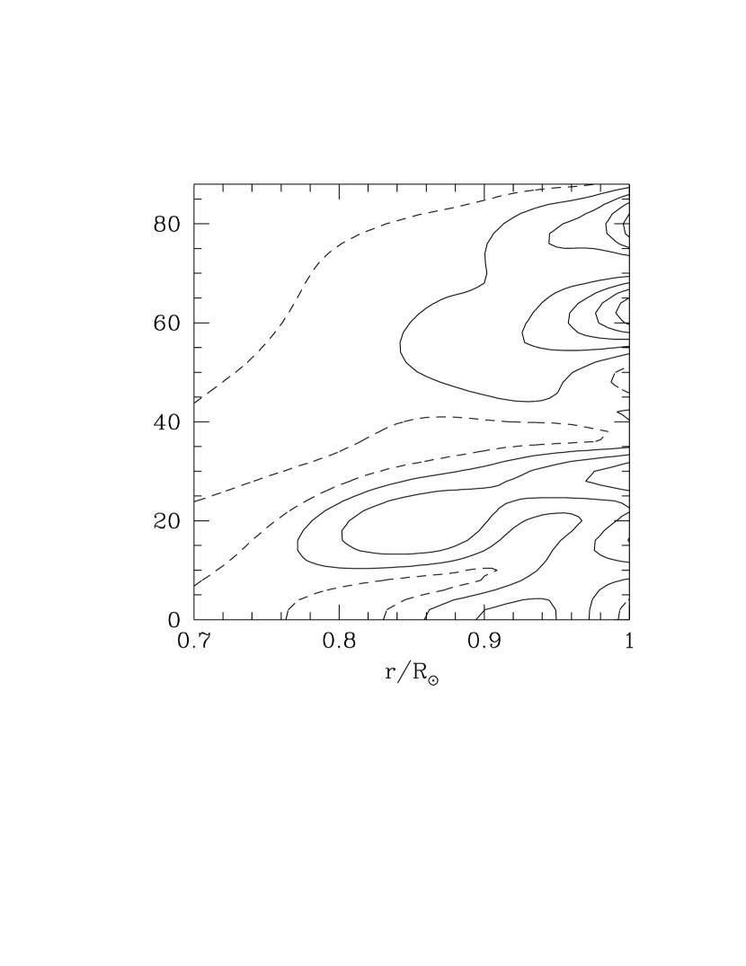
Figure 4: Contour diagram showing amplitudes of the $k=1$ and $k=3$ (Eq. 8) components of zonal flow expansion as obtained using GONG data, assuming a period of 11 years. The contours are at intervals of 1 m/s with dashed contour representing the value of 1 m/s. The left panel shows $a_{1}$ while the right panel shows $a_{3}$.

where $\omega=2\pi/11$ yr^-1 is the basic frequency of the solar cycle. Here $a_{k}$ is the amplitude of $k$th harmonic and $\phi_{k}$ its phase. Since we have data over only a part of the solar cycle, different components in Eq. 8 are not orthogonal and their relative amplitudes depend on which components are included in the fit. We find that inclusion of $k=2$ component tends to suppress the amplitude of the fundamental ($k=1$) component, while inclusion of the $k=3$ component does not affect the amplitude of $k=1$ component. To illustrate the results Fig. 4 shows contour diagrams for the amplitudes of the $k=1$ and 3 components, when only components for $k=1,3,5$ are used in the fit. The first component is qualitatively similar to that found by Vorontsov et al. (2002) who also find a prominent feature extending through most of the convection zone at high latitudes. At middle latitudes of around $45^{\circ}$ the amplitude is small. At low latitudes again it is clear that the pattern penetrates to depths close to the base of the convection zone as inferred above from the study of radial behavior of the zonal flow velocities. It is clear that the $k=3$ harmonic is significant, though its magnitude is about half of the first term. Vorontsov et al. (2002) also find the third harmonic in their analysis. The significant amplitude of higher components may be expected from the non-sinusoidal form of the temporal variation. It could also arise if the basic period is different from 11 years. From the limited data that we have, we cannot distinguish between these possibilities. The relative magnitude of various harmonics will depend on the origin of the zonal flow pattern. Below the convection zone the amplitude of the main component is very small, indicating that solar cycle variations are not seen in these layers. At very deep layers, close to the tachocline, the errors on the zonal flow velocities are so large, that we cannot assign any significance to the fluctuating results obtained there.

3.2 The tachocline

To study possible temporal variations in the properties of the tachocline, we use each of the non-overlapping data sets from the GONG and MDI to determine the mean location, width and the jump in the rotation rate across the tachocline. To improve the precision of the results, we take the weighted mean of the values obtained using the three methods mentioned in §2.1. Each result is weighted inversely with the square of the estimated error while calculating the mean value. Fig. 5 shows the position and the half-width of the tachocline as a function of time for both the GONG and MDI data. Note that while taking averages the errors have been estimated by assuming that there is no correlation between different estimates. This may, in principle, cause the errors to be underestimated. However, looking at the scatter between different points in Fig. 5 it appears that errors may actually be overestimated, particularly at high latitudes. This could be due to correlation between different tachocline parameters in our fits. It can be seen that none of these properties show any significant temporal variation. There appears to be some systematic difference between GONG and MDI results for depth of the tachocline at high latitude. This could be due to known differences between the two data sets (e.g., Howe et al. 2001b; Schou et al. 2002) which mainly arise from differences in the data reduction techniques. The variation in $\delta\Omega_{t}$ is not shown in the figure, but that also does not show any clear temporal variations.

Since we do not find any significant temporal variations in the properties of the tachocline, we can take the temporal average of all sets to improve the precision of the results, and the averages at a few latitudes are shown in Table 2. These averages are obtained by combining all non-overlapping sets in both the GONG and MDI data. From this table it is clear that there is a distinct latitudinal variation in the position and thickness of the tachocline. These results are consistent with those of Charbonneau et al. (1999) and Basu & Antia (2001). However, it appears that the latitudinal variations in the position and width may not be continuous. The position and width at latitudes of $0^{\circ}$ and $15^{\circ}$ are the same within error bars. Similarly, those at latitudes of $45^{\circ}$ and $60^{\circ}$ are close to each other. In between these pairs of latitudes, is the transition in the sign of $\delta\Omega_{t}$, the jump in rotation rate across the tachocline. At low latitudes the rotation rate increases with radial distance, while at high latitudes the rotation rate decreases with radial distance in the tachocline. Thus it is possible that the tachocline consists of two parts one at low latitudes and the other at high latitudes which are located at different depths and have different widths, but there may be no variation in position and width within each of these regions. Fig. 6 shows such a representation of the tachocline. In this figure we have used a half-width of $2.5w$ to cover the region where $85\%$ of the transition in rotation rate is complete. This is equivalent to the width of the tachocline as defined by Kosovichev (1996) and Charbonneau et al. (1999). At the base of the convection zone the latitudinal resolution of observed frequency splittings is limited and from these results it is not possible to decide if there is indeed a discontinuity in the tachocline properties as a function of latitude or whether the variation is gradual between latitudes of $15^{\circ}$ and $45^{\circ}$. If the variation is confined to a very narrow latitude range than for all practical purposes it can be considered as a discontinuity. Clearly, more work is needed to confirm whether the latitudinal variation is indeed steep around a latitude of $30^{\circ}$.

In order to test if there is indeed a discontinuity in the position and width of the tachocline as a function of latitude, we repeat the 2d simulated annealing fit to the tachocline properties assuming a discontinuity in $r_{d}$ and $w$ at $\theta=30^{\circ}$. The difference in $\chi^{2}$ per degree of freedom for fits with discontinuity and those with continuous variation with $\theta$ is shown as a function of time in Fig. 7. The GONG data appears to favor a discontinuity, though the difference in $\chi^{2}$ is rather small. The MDI data do not show any clear difference. On average for MDI results, the $\chi^{2}$ increases in the presence of discontinuity, and thus these results do not favor discontinuity in latitudinal dependence, but the scatter in MDI points is much larger than those in GONG points. Moreover, there appears to be some systematic increase in $\delta\chi^{2}$ between the pre- and post-recovery data sets from MDI. It is not clear if this is due to possible systematic errors due to variations in MDI characteristics during recovery (Antia 2002) or a temporal variation or simply statistical fluctuation. We do not know why this difference in behavior is seen between the GONG and MDI results. The GONG data also show a distinct temporal variation in the $\chi^{2}$ difference, thus suggesting that there may be a temporal variation in the magnitude of the discontinuity at $\theta=30^{\circ}$. Fig. 8 shows the position of the tachocline in the two regions as a function of time as obtained using the GONG data. There is a very marginal variation in the position of the tachocline at high latitudes, which is within error bars. This figure can be compared with Fig. 5 which shows the same results using other techniques. Note that in both Figs. 5 and 8 the scatter in position is much less at high latitudes. In Fig. 8 this is clearly due to the correlation between $r_{t}$ and $\delta r_{t}$ which can be verified by looking at the fits to these two parameters. A similar correlation is present in the fits to the continuous function too, resulting in smaller scatter at high latitudes, which leads to an overestimate of errors. It is not clear if this temporal variation is significant. If this variation is real, it will imply that the high latitude part of the tachocline moves up or down with the solar activity and this movement may play a crucial role in the operation of dynamo. The corresponding variation in the width is not clear at all.

3.3 North-South asymmetry in the rotation rate

To study the north-south antisymmetric component of the rotation rate we use the ring diagram technique. The inverted values of $u_{x}$ contain information about the rotation rate in the solar interior. Since the rate at which the regions were tracked is symmetric about the equator, any difference between the inverted $u_{x}$ at a given latitude of the northern hemisphere and that at the same latitude in the southern hemisphere is caused by the asymmetry of the rotation rate about the equator.

The north-south antisymmetric component of the rotation velocity at various times are shown in Fig. 9 at two sample radii. The component appears to change somewhat with time, however, it is not clear if there is any systematic temporal variation. It is possible that we have to look at intermediate time-steps to discern any pattern. Alternatively, it is possible that the apparent variations are caused by errors in pointing or tracking, and/or errors in inversions. In the outer layers, above a radius of about $0.98R_{\odot}$, the antisymmetric component appears to be significant. An average over all data sets shows a significant slope in these layers. Below this depth the errors in inferred velocity are too large to make any definite conclusion.

3.4 The meridional flow

The meridional flow velocity, $u_{y}$, at two representative depths is shown as a function of latitude in Fig. 10. The results of all eight data sets are shown. The dominant component in meridional velocity is the north-south anti-symmetric component with a variation of form $\sin(2\theta)$. In both hemispheres the meridional flow is from equator towards the poles. The meridional flow shows a definite, and systematic time variation. The maximum velocity of the flow is smaller when the Sun is more active. There is a small southward flow at the equator at all times, but that could be an artifact of pointing errors or errors in the Carrington elements used to define the rotation axis or other systematic errors in the ring diagram analysis, and as such its significance is difficult to ascertain. This southward flow was also seen by Giles et al. (1997) and Basu et al. (1999). We note that the expected ‘S’ shape of the flow is seen only at very shallow depths. At deeper layers, the data sets from low activity period do not show any tendency of lowering velocity at high latitudes, while the data sets during high activity period do. The time variation is seen more clearly if we plot the north-south antisymmetric component of the flow, which is shown in Fig. 11. In this figure the decrease in velocity at high latitudes with time can be clearly seen. The flow speeds at low latitudes show almost no change with time, the intermediate and high latitudes do.

To take a more detailed look at the meridional flow variations we decompose the flow velocity into different components (see Hathaway et al. 1996):

$$u_{y}(r,\phi)=-\sum_{i}a_{i}(r)P^{1}_{i}(\cos(\phi)),$$ (9)

where $\phi$ is the colatitude, $P^{1}_{i}(x)$ are the associated Legendre functions. The first six components are found to be significant and are shown in Fig. 12. These components also show a variation with time. For most of these components the temporal variation is not systematic, and could be due to errors in estimating their amplitudes. We plot the amplitudes of the different components as a function of time at a sample radius of $r=0.995R_{\odot}$ in Fig. 13. We can see clearly that only the amplitude of the dominant component, $a_{2}$, shows a systematic variation with time, with its magnitude reducing with time during the time period covered by the MDI data. The north-south symmetric component $a_{1}$ is not zero, and always shows a south-wards flow. It does show a change with time, but it is difficult to say whether it is real, since a changing pointing-error would give a similar result. The symmetric component $a_{3}$ is also non-zero, but again its significance is hard to judge. The higher order components do not seem to show significant temporal variation. Other than $a_{2}$ and perhaps $a_{1}$, no component seems to show a definite change with time either. Similar results are found at radii larger than $0.99R_{\odot}$, but in deeper layer no systematic temporal variation is seen in any of these components.

4 DISCUSSION AND CONCLUSIONS

We have done a comprehensive analysis of the available helioseismic data from the GONG and MDI projects to study changes in the solar dynamics with changes in the level of solar activity. The rotation-rate residuals obtained by subtracting the time-averaged rotation rate from that at each epoch show the well-known pattern of zonal flows similar to the torsional oscillations observed at the surface. This pattern consists of bands of faster and slower than average rotation rate moving towards the equator with time at low latitudes. At high latitudes these bands move towards the poles. The transition between equator-ward and pole-ward movement occurs around a latitude of $50^{\circ}$. Observations of magnetic features at the solar surface also show similar pole-ward movement at high latitudes (cf., Leroy & Noens 1983; Makarov & Sivaraman 1989; Erofeev & Erofeeva 2000; Benevolenskaya et al. 2001). Theoretical models of Covas et al. (2000, 2001) using a mean-field dynamo also show this feature.

The zonal flow pattern at low latitudes appears to be rising upwards with time at a rate of about 1 m/s at low latitudes. A similar conclusion was drawn by Komm, Howard & Harvey (1993) by comparing the zonal flow pattern obtained using the Doppler measurements at the surface with those from magnetic features which are believed to be anchored below the surface. Furthermore, from the variation with depth it appears that the zonal flows penetrate through a good fraction of the convection zone. This appears to contradict earlier inferences (Howe et al. 2000a; Antia & Basu 2000) that these flows penetrate to a radius of $0.9R_{\odot}$ only. This difference may be because the errors in inversion increase with depth thus making it difficult to decide whether the pattern continues to deeper layers. Particularly, at high latitudes the errors are large and it may be difficult to see the pattern in deeper layers. In these earlier works an attempt was made to look at the pattern at a range of latitudes and that may be the reason that it was difficult to verify if it penetrates through the convection zone. If we look only at low latitudes where errors are comparatively small, it appears that the pattern penetrates deeper. Recently, Vorontsov et al. (2002) also found that a band of faster rotating elements appear to penetrate almost up to the base of the convection zone at latitude of around $60^{\circ}$. We also find similar results at this latitude. The mean-field dynamo models of Covas et al. (2000, 2001) also predict that the zonal flow pattern should persist through the convection zone. Our results suggest that this is likely to be true, though at high latitudes the situation is not clear. More data covering the entire solar cycle may be able to resolve this issue.

It is conventionally assumed that the solar dynamo is located in the tachocline region below the base of the convection zone, and hence, one would expect changes there. However, we do not find any significant temporal variation in the properties of the tachocline. A temporal mean over all data though shows a clear latitudinal variation in the depth and thickness of the tachocline. Similar latitudinal variations have been seen earlier (Charbonneau et al. 1999; Basu & Antia 2001). A closer look at this variation suggests that the tachocline may consist of two parts, one at low latitudes where the rotation rate increases with radial distance and other at high latitudes where the rotation rate decreases with $r$. These parts appear to have different depth and thickness, but there may not be much latitudinal variation within each of these parts. On the other hand, it is known that there is no significant latitudinal variation in the depth of the convection zone (Basu & Antia 2001). Similarly, any possible latitudinal variation in sound speed at the base of the convection zone is less than $10^{-4}$ (Antia et al. 2001). The latitudinal variation in the position of the tachocline is however highly significant, being $(0.019\pm 0.003)R_{\odot}$. It is generally believed that shear within the tachocline gives rise to some mixing which accounts for the low lithium abundance on the solar surface as well as the bump in sound speed difference seen in solar models which do not include this mixing (Christensen-Dalsgaard et al. 1996). Inclusion of mixing in the tachocline removes the bump (Richard et al. 1996; Brun, Turck-Chièze & Zahn 1999). Thus if the position and thickness of the tachocline depend on the latitude, the extent of mixing should also depend on the latitude which should give rise to a strong latitudinal variation in the solar structure. However, we do not see any evidence for significant latitudinal variation in the solar structure. This would imply that the tachocline cannot be responsible for mixing, unless the depth and thickness of the tachocline vary in such a manner that the lower boundary of the mixed region is essentially independent of the latitude. From Fig. 6 it can be seen that this is indeed the case, with the lower boundary of the tachocline being essentially independent of latitude. Of course, the thickness of $2.5w$ is chosen to achieve this purpose, but it is a reasonable estimate of the mixing region. Thus if the thickness of the tachocline varies along with the depth in a suitable manner it may be possible to ensure that the solar structure is close to being spherically symmetric. From this point of view also it is simpler to assume that the tachocline consists of two parts, rather than assuming that it has a continuous latitudinal variation. In the latter case one will require the thickness to match the latitudinal variation in depth at every latitude.

It may be argued that we will need some coincidence to match the variation in depth and latitude even with a two component model for the tachocline. It may be noted that in the absence of any mixing, the squared sound speed in a solar model departs by about 0.5% from the solar values as inferred by inversions (Christensen-Dalsgaard et al. 1996) while the latitudinal variation in the sound speed in the tachocline region is less than a few parts in $10^{5}$. It is not clear what causes this agreement between depth and thickness variations. From Fig. 6 it appears that at low latitudes the upper limit of the tachocline is below the base of the convection zone and hence there could be some region which is not fully mixed. This difference is very small and could be a result of errors in the deduced values of the tachocline position or thickness. A very thin layer that is not fully mixed may not result in any significant anomaly in the solar structure.

To test the two component hypothesis for the tachocline, we attempt a 2d simulated annealing fit with discontinuity in latitude for position and width. The fits to the GONG data show a marginal reduction in $\chi^{2}$ per degree of freedom when discontinuity is introduced in latitudinal variation. It may be noted that the number of parameters to be fitted is the same in both continuous and discontinuous case. This result is not confirmed by the MDI data which do not show any systematic differences in $\chi^{2}$. The reason for this discrepancy is not understood. The GONG data also indicate that the position of the tachocline at high latitude may be moving upward with activity. The temporal variation is less than $1\sigma$ error bars and its significance is not clear.

The north-south antisymmetric component of rotation rate cannot be detected from the splittings of global modes. We use the ring diagram technique to study this component in the outer convection zone. We do not find any definite temporal variation in this component. Averaging over time we find this component to be significant above $r=0.98R_{\odot}$, where it has a magnitude of about 5 m/s at a latitude of $45^{\circ}$. It is quite possible that this is an artifact of systematic errors in ring diagram analysis.

The meridional component of velocity can also be studied using the ring diagram technique. The meridional flow velocity shows a clear temporal variation as its magnitude seems to decrease with increase in the solar activity. The dominant component of the meridional flow velocity, i.e., $1.5a_{2}\sin(2\theta)$ shows a systematic decrease in amplitude with time during the period 1996–2002. The temporal variation in the rotation rate and meridional flow should provide constraints on dynamo models. Haber et al. (2002) have also studied temporal variation in the meridional flow pattern using ring diagram analysis. Their results also suggest that there may be reduction in meridional velocity with activity. They have claimed to detect an occurrence of submerged meridional cell in the northern hemisphere. We do not find this pattern in our results and the cause of this discrepancy is not clear. Haber et al. (2002) also find that the latitudinal gradient of the meridional flows near the equator steepens with time, this is not clear in our work. More work is needed to study possible systematic errors in ring diagram analysis before it can be used to study small temporal variations reliably. In particular, the flow pattern is likely to be modified in the vicinity of active regions and presence of large number of active regions during high activity period can modify the inferences even when average over a large number of regions is taken to find the mean meridional flow velocity.

While discussing the time variability of the meridional flow or the north-south antisymmetric component of the zonal flow, one should keep in mind that any time variations in the instrument properties will result in a spurious time variation of the flows. This is less true for symmetric component of zonal flows since global modes are not affected as much. The zonal flow results are also confirmed by using two different sets of data (GONG and MDI), while in the case of the meridional flows we have only used the MDI data. It would be interesting to verify these results using GONG+ data that is now becoming available. There is some evidence that some systematic error may have been introduced in the MDI data during recovery of the SOHO satellite (Antia 2002). It is not clear how this will affect the meridional flow measurements.

Table 1: Regions studied

No.	Carr.	No. of	Lon.	Time	10.7cm
	Rot.	spectra			Flux
1	1911	12	285-120	1996.07	$70.5\pm 0.5$
2	1921	08	120-015	1997.04	$71.4\pm 0.5$
3	1932	09	360-240	1998.02	$84.8\pm 1.3$
4	1948	24	360-015	1999.04	$120.4\pm 2.5$
5	1964	24	360-015	2000.06	$188.9\pm 3.8$
6	1975+76	24	120-135	2001.04-5	$154.1\pm 3.2$
7	1985	15	300-075	2002.01	$224.0\pm 3.4$
8	1988	24	360-15	2002.03-4	$197.2\pm 2.9$

Table 2: Properties of the tachocline at a few selected latitudes: All quantities are the weighted averages of the results obtained by all three techniques mentioned in Section 1.2 from all the non-overlapping data sets from GONG and MDI. It is assumed that the different measurements are uncorrelated.

Latitude	$\delta\Omega_{t}$	$r_{t}$	$w$
(∘)	(nHz)	($R_{\odot}$)	($R_{\odot}$)
0	$\phantom{-}20.82\pm 0.43$	$0.6916\pm 0.0019$	$0.0065\pm 0.0013$
15	$\phantom{-}17.83\pm 0.24$	$0.6909\pm 0.0018$	$0.0078\pm 0.0013$
45	$-30.54\pm 0.54$	$0.7096\pm 0.0019$	$0.0103\pm 0.0012$
60	$-67.65\pm 0.74$	$0.7104\pm 0.0022$	$0.0151\pm 0.0020$

Figure 1: Contour diagrams of constant rotation velocity residuals at $r=0.98R_{\odot}$ obtained using 2D RLS inversion of the GONG data. The continuous contours are for positive $\delta v_{\phi}$, while dotted contours denote negative values. The contours are drawn at interval of 1 m/s and the zero contour is not shown.

Figure 2: The rotation-velocity residuals from the GONG data as a function of time and radial distance at selected latitudes. The contours of constant residual velocity are shown at intervals of 1 m/s, with continuous contours showing positive values and dotted contours showing negative values. The zero contour is not shown.

Figure 3: The zonal flow velocity as a function of time at different latitudes at $r=0.98R_{\odot}$. The latitudes are marked in each panel. The solid line shows the GONG results, while points with error bars show the MDI results.

Figure 5: The mean radial position and half-width of the tachocline at a latitude of $15^{\circ}$ and $60^{\circ}$ is shown as a function of time for the GONG (crosses) and MDI (squares) data. These results are weighted averages of those obtained using the three techniques mentioned in §2.1.

Figure 6: The location of the tachocline inside the Sun. The shaded area is the tachocline with a half-width of $2.5w$. The dashed line shows the base of the convection zone at $r=0.713R_{\odot}$ (Christensen-Dalsgaard, Gough & Thompson 1991; Basu & Antia 1997).

Figure 7: The difference in $\chi^{2}$ per degree of freedom between 2d fits to the continuous functions and those to functions with discontinuity in latitude.

Figure 8: The tachocline position as obtained from 2d fits to a function with discontinuity in $\theta$ to the GONG data. The left panel shows the results at low latitude while the right panel shows the results for high latitudes.

Figure 9: The North-South antisymmetric component of the solar rotation velocity as a function of latitude at two different radii. Only OLA results are shown. RLS results are very similar. These results were obtained by the ring-diagram analysis of MDI data.

Figure 10: The meridional flow velocities obtained from the different data sets plotted as a function of latitude for two different radii. Only OLA results are shown. RLS results are very similar.

Figure 11: The north-south antisymmetric component of meridional flow velocities obtained from the different data sets plotted as a function of latitude for two different radii. Only OLA results are shown. RLS results are very similar.

Figure 12: The amplitude of the different components of the meridional flow as defined in Eq. (9) plotted as a function of radius. The different line types represent the different data sets (see legend of Figs. 10 and 11). Only RLS results are shown, OLA results are very similar. The error bars are not shown for clarity, but these can be seen in Fig. 13.

Figure 13: The amplitudes of the different components of the meridional flow plotted as a function of time at $r=0.995R_{\odot}$.

References

- Anderson et al. (1990) Anderson, E. R., Duvall, T. L., Jr., & Jefferies, S. M. 1990, ApJ, 364, 699
- Antia (2002) Antia, H. M. 2002, in Magnetic Coupling of the Solar Atmosphere, Proc. IAU Coll. 188 (ESA SP-505; Noordwijk: ESA) (in press) (astro-ph/0208339)
- Antia & Basu (2000) Antia, H. M., & Basu, S. 2000, ApJ, 541, 442
- Antia & Basu (2001) Antia, H. M., & Basu, S. 2001, ApJ, 559, L67
- ANtia, Basu, & Chitre (2001) Antia, H. M., Basu, S., & Chitre, S. M. 1998, MNRAS, 298, 543
- Antia et al. (2001) Antia, H. M., Basu, S., Hill, F., Howe, R., Komm, R. W., & Schou, J. 2001, MNRAS, 327, 1029
- Basu (2002) Basu, S. 2002, in From Solar Minimum to Maximum: Half a Solar Cycle with SOHO, Proc. SOHO11 Workshop, ed. A. Wilson (ESA SP-508; Noordwijk: ESA), 7
- Basu & Antia (1997) Basu, S., & Antia, H. M. 1997, MNRAS, 287, 189
- Basu & Antia (1999) Basu, S., & Antia, H. M. 1999, ApJ, 525, 517
- Basu & Antia (2000a) Basu, S., & Antia, H. M. 2000a, Sol. Phys., 192, 449
- Basu & Antia (2000b) Basu, S., & Antia, H. M. 2000b, Sol. Phys., 192, 469
- Basu & Antia (2001) Basu, S., & Antia, H. M. 2001, MNRAS, 324, 498
- Basu, Antia & Tripathy (1999) Basu, S., Antia, H. M., & Tripathy, S. C. 1999, ApJ, 512, 458
- Benevolenskaya, Kosovichev & Scherrer (2001) Benevolenskaya, E. E., Kosovichev, A. G., & Scherrer, P. H. 2001, ApJ, 554, L107
- Bogart et al. (1997) Bogart, R. S., et al. 1997, in Sounding Solar and Stellar Interiors, IAU Symposium 181, eds. J. Provost & F.-X. Schmider, Kluwer Academic Publishers, 111
- Bogart, Basu & Antia (2002) Bogart, R. S., Basu, S., & Antia, H. M. 2002, in From Solar Minimum to Maximum: Half a Solar Cycle with SOHO, Proc. SOHO11 Workshop, ed. A. Wilson (ESA SP-508; Noordwijk: ESA), 145
- Brown et al. (1989) Brown, T. M., Christensen-Dalsgaard, J., Dziembowski, W. A., Goode, P., Gough, D. O., & Morrow, C. A. 1989, ApJ, 343, 526
- Brun & Toomre (2001) Brun, A. S., & Toomre, J. 2001, in Helio- and Astero-seismology at the Dawn of the Millennium, ed. A. Wilson, (ESA SP-464; Noordwijk: ESA), 619
- Brun, Turck-Chièze & Zahn (1999) Brun, A. S., Turck-Chièze, S., & Zahn, J. P. 1999, ApJ, 525, 1032
- Charbonneau et al (1999) Charbonneau, P., Christensen-Dalsgaard, J., Henning, R., Larsen, R. M., Schou, J., Thompson, M. J., & Tomczyk, S. 1999, ApJ, 527, 445
- Christensen-Dalsgaard & Schou (1988) Christensen-Dalsgaard, J., & Schou, J. 1988, in Seismology of the Sun and Sun-like Stars, ed. E.J.Rolfe (ESA SP-286; Noordwijk: ESA), 149
- Christensen-Dalsgaard et al. (1991) Christensen-Dalsgaard, J., Gough, D. O., & Thompson, M. J. 1991, ApJ, 378, 413
- Christensen-Dalsgaard et al. (1996) Christensen-Dalsgaard, J., et al. 1996, Sci., 272, 1286
- Corbard et al. (2001) Corbard, T., Jiménez-Reyes, S. J., Tomczyk, S., Dikpati, M., & Gilman, P. 2001, in Helio- and Astero-seismology at the Dawn of the Millennium, ed. A. Wilson (ESA SP-464; Noordwijk: ESA), 265
- Covas et al. (2000) Covas, E., Tavakol, R., Moss, D., & Tworkowski, A. 2000, A&A, 360, L21
- Covas et al. (2001) Covas, E., Tavakol, R., & Moss, D. 2001, A&A, 371, 718
- Dikpati & Charbonneau (1999) Dikpati, M., & Charbonneau, P. 1999, ApJ, 518, 508
- Dikpati & Gilman (2001) Dikpati, M., & Gilman, P. 2001, ApJ, 559, 428
- Elsworth et al¿ (1990) Elsworth, Y., Howe, R., Isaak, G. R., McLeod, C. P., & New, R. 1990, Nature, 345, 322
- Erofeev & Erofeeva (2000) Erofeev, D. V., & Erofeeva, A. V. 2000, Sol. Phys., 191, 281
- Giles et al. (1997) Giles, P. M, Duvall, T. L., Jr., Scherrer, P. H., & Bogart, R. S. 1997, Nature, 390, 52
- Haber et al. (2001) Haber, D. A., Hindman, B. W., Toomre, J., Bogart, R. S., & Hill, F. 2001, in Helio- and Astero-seismology at the Dawn of the Millennium, ed. A. Wilson (ESA SP-464; Noordwijk: ESA), 209
- Haber et al. (2002) Haber, D. A., Hindman, B. W., Toomre, J., Bogart, R. S., Larsen, R. M., & Hill, F. 2002, ApJ, 570, 855
- Hathaway et al. (1996) Hathaway, D. H., et al. 1996, Sci., 272, 1306
- Hill (1988) Hill, F. 1988, ApJ, 333, 996
- Hill et al. (1996) Hill, F., et al. 1996, Sci., 272, 1292
- Howard & LaBonte (1980) Howard, R., & LaBonte, B. J. 1980, ApJ, 239, L33
- Howe et al. (2000a) Howe, R., Christensen-Dalsgaard, J., Hill, F., Komm, R. W., Larsen, R. M., Schou, J., Thompson, M. J., & Toomre, J. 2000a, ApJ, 533, L163
- Howe et al. (2000b) Howe, R., Christensen-Dalsgaard, J., Hill, F., Komm, R. W., Larsen, R. M., Schou, J., Thompson, M. J., & Toomre, J. 2000b, Sci, 287, 2456
- (40) Howe, R., Christensen-Dalsgaard, J., Hill, F., Komm, R. W., Larsen, R. M., Schou, J., Thompson, M. J., & Toomre, J. 2001a, in Helio- and Asteroseismology at the Dawn of the Millennium, ed. A. Wilson (ESA SP-464; Noordwijk: ESA), 19
- Howe et al. (2001b) Howe, R., Hill, F., Basu, S., Christensen-Dalsgaard, J., Komm, R. W., Larsen, R. M., Roth, M., Schou, J., Thompson, M. J., & Toomre, J. 2001b, in Helio- and Astero-seismology at the Dawn of the Millennium, ed. A. Wilson (ESA SP-464; Noordwijk: ESA), 137
- Jiménez-Reyes et al. (2001) Jiménez-Reyes, S. J., Corbard, T., Pallé, P. L., Roca Cortés, T., & Tomczyk, S. 2001, A&A, 379, 622
- Komm, Howard & Harvey (1993) Komm, R. W., Howard, R. F., & Harvey, J. W. 1993, Sol. Phys., 143, 19
- Korzennik, Rabello-Soares & Schou (2002) Korzennik, S. G., Rabello-Soares, M. C., & Schou, J. 2002, (astro-ph/0207371)
- Kosovichev (1996) Kosovichev, A. G. 1996, ApJ, 469, L61
- Kosovichev et al. (1997) Kosovichev, A. G., et al. 1997, Sol. Phys., 170, 43
- LaBonte & Howard (1982) LaBonte, B. J., & Howard, R. 1982, Sol. Phys., 75, 161
- LeRoy & Noens (1983) Leroy, J. -L., & Noens, J. -C. 1983, A&A, 120, L1
- Libbrecht (1989) Libbrecht, K. G. 1989, ApJ, 226, 1092
- Libbrrecht & Woodard (1990) Libbrecht, K. G., & Woodard, M. F. 1990, Nature, 345, 779
- Makarov & Sivaraman (1989) Makarov, V. I., & Sivaraman, K. R. 1989, Sol. Phys., 123, 367
- Miesch (2000) Miesch, M. 2000, Sol. Phys., 192, 59
- Nandy & Choudhuri (2002) Nandy, D., & Choudhuri, A. R. 2002, Sci., 296, 1671
- Nigam & Kosovichev (1998) Nigam, R., & Kosovichev, A. G. 1998, ApJ, 505, L51
- Patrón et al. (1997) Patrón, J., et al. 1997, ApJ, 485, 869
- Rajaguru, Basu & Antia (2001) Rajaguru, S. P., Basu, S., & Antia, H. M. 2001, ApJ, 563, 401
- Richard et al. (1996) Richard, O., Vauclair, S., Charbonnel, C., & Dziembowski, W. A. 1996, A&A, 312, 1000
- Rhodes et al. (1998) Rhodes, E. J., Jr., Reiter, J., Kosovichev, A. G., Schou, J., & Scherrer, P. H. 1998, in Structure and Dynamics of the Interior of the Sun and Sun-like Stars: Proc. SOHO 6/GONG 1998 Workshop, ed. S. Korzennik & A. Wilson (ESA SP-418; Noordwijk: ESA), 73
- Ritzwoller & Lavely (1991) Ritzwoller, M. H., & Lavely, E. M. 1991, ApJ, 369, 557
- Schou, Christensen-Dalsgaard & Thompson (1994) Schou, J., Christensen-Dalsgaard, J., & Thompson, M. J. 1994, ApJ, 433, 389
- Schou (1999) Schou, J. 1999, ApJ, 523, L181
- Schou et al. (1998) Schou, J., et al. 1998, ApJ, 505, 390
- Schou et al. (2002) Schou, J., et al. 2002, ApJ, 567, 1234
- Snodgrass (1984) Snodgrass, H. B. 1984, Solar Phys., 94, 13
- Snodgrass (1992) Snodgrass, H. B. 1992, in The Solar Cycle, Proc. NSO 12th Summer Workshop, ASPS 27, 205
- Spiegel & Zahn (1992) Spiegel, E. A., & Zahn, J.-P. 1992, A&A, 265, 106
- Thompson et al. (1996) Thompson, M. J., et al. 1996, Sci., 272, 1300
- Toomreet al. (2000) Toomre, J., Christensen-Dalsgaard, J., Howe, R., Larsen, R. M., Schou, J., & Thompson, M. J. 2000, Sol. Phys., 192, 437
- Ulrich (2001) Ulrich, R. K. 2001, ApJ, 560, 466
- Ulrich (1988) Ulrich, R. K., Boyden, L. W., Snodgrass, H. B., Padilla, S. P., Gilman, P., & Shieber, T. 1988, Sol. Phys., 117, 291
- Vorontsov (2001) Vorontsov, S. V. 2001, in Helio- and Astero-seismology at the dawn of the millennium: Proc. SOHO 10/GONG 2000 Workshop, ed. A. Wilson (ESA SP-464; Noordwijk: ESA), 563
- Vorontsov (2002) Vorontsov, S. V. 2002, in From Solar Minimum to Maximum: Half a Solar Cycle with SOHO, Proc. SOHO11 Workshop, ed. A. Wilson (ESA SP-508; Noordwijk: ESA), 107
- Vorontsov et al. (2002) Vorontsov, S. V., Christensen-Dalsgaard, J., Schou, J., Strakhov, V. N., & Thompson, M. J. 2002, Sci., 296, 101
- Woodard (2000) Woodard, M. F. 2000, Sol. Phys., 197, 11