Star Formation and Metallicity History of the SDSS galaxy survey: unlocking the fossil record

Abstract

Using MOPED we determine non-parametrically the star-formation and metallicity history of over 37,000 high-quality galaxy spectra from the Sloan Digital Sky Survey (SDSS) early data release. We use the entire spectral range, rather than concentrating on specific features, and we estimate the complete star formation history without prior assumptions about its form (by constructing so-called ‘population boxes’). The main results of this initial study are that the star formation rate in SDSS galaxies has been in decline for $\sim$ 6 Gyr; a metallicity distribution for star-forming gas which is peaked $\sim 3$ Gyr ago at about solar metallicity, inconsistent with closed-box models, but consistent with infall models. We also determine the infall rate of gas in SDSS and show that it has been significant for the last 3 Gyr. We investigate errors using a Monte-Carlo Markov Chain algorithm. Further, we demonstrate that recovering star formation and metallicity histories for such a large sample becomes intractable without data compression methods, particularly the exploration of the likelihood surface. By exploring the whole likelihood surface we show that age-metallicity degeneracies are not as severe as by using only a few spectral features. We find that 65% of galaxies contain a significant old population (with an age of at least 8 Gyr), including recent starburst galaxies, and that over 97% have some stars older than 2 Gyr. It is the first time that a complete star formation and metallicity history, without restrictive assumptions about its form have been derived for such a large dataset of integrated stellar populations, and the first time that the past star formation history has been determined from the fossil record of the present-day spectra of galaxies.

1 Introduction

The measured spectrum of a galaxy contains, in principle, information about the physical processes that led to its formation and evolution. The amount of gas transformed into stars, the metallicity of that gas and the dust produced in it at a given time all affect the integrated light of a galaxy. Therefore, nearby spectra should contain a precious fossil record about the conditions of the interstellar medium in the past, and can be compared to methods based on measurements of recent star formation activity, measured at different redshifts (cf Lilly et al. (1996); Madau et al. (1996); Hughes et al. (1998); see also Baldry et al. (2002)). The challenge is to recover all the information contained in the spectrum. In principle, this is not a difficult task since the composite spectrum of a stellar population will be just the sum of single stellar population spectra over the history of the galaxy. An essentially non-parametric reconstruction of the star formation history and metallicity can be achieved by searching for the best-fitting model. This can easily be attempted for a small number spectra using the whole data set of measured fluxes, with weak constraints on the star formation history, such as piecewise continuity. Despite its simplicity, this approach has never been used and it is most common to assume a very simple parametrisation of the star formation (usually a declining exponential with the amplitude and decay time as parameters) and a given metallicity history. In addition, most of the analysis is usually done on pre-selected features (absorption or emission lines) of the spectrum. This limits the amount of information that can be extracted and also introduces artificial degeneracies among the parameters that could be lifted using all information in the spectrum.

More sophisticated approaches to recover physical information from galaxy spectra than simply using a pre-selected set of spectral features or broad-band colours have been used in the literature. Many of these are based on principal component analysis (PCA) or wavelet decomposition (e.g. Murtagh & Heck (1987); Francis et al. (1992); Connolly et al. (1995); Ronen et al. (1999); Folkes et al. (1999); Madgwick et al. (2002)), based on information theory (Slonim et al., 2000) or solving the inverse problem (Vergely, Lancon & Mouchine, 2002). However, when dealing with large datasets, like SDSS, with potentially 10⁶ spectra, it is impractical to use all of the flux data for every galaxy - searching for the best fitting model for a spectrum with 10,000 flux points takes about an hour on a high-end PC linux work station. Data compression of some sort is necessary, and this can be achieved by concentrating on particular stellar features, such as the 4000Å break and $H\delta$, plus broad-band colours (Kauffmann et al., 2002). The approach of MOPED (Multiple Optimised Parameter Estimation and Data compression; (Heavens, Jimenez & Lahav, 2000)) is rather different. It chooses a relatively small number of linear combinations of the data, where the weightings are chosen carefully and automatically to preserve as much information as possible about the parameters one wants to know about (the star formation and metallicity histories, and the dust content). In this way it is possible in a practical way to recover virtually as much information as is theoretically possible, given the data and a theoretical model.

In this paper we use the radical data compression algorithm MOPED to greatly reduce the time that is needed to find a best-fitting model. This algorithm allows us to obtain an essentially non-parametric reconstruction of the star formation and metallicity histories of the galaxies in the early data release of the Sloan Digital Sky Survey (SDSS). As important as the results obtained is the fact that the fast algorithm allows us to explore the likelihood surface and obtain realistic errors. We have previously shown the potential of MOPED with a very modest sample (Reichardt, Jimenez & Heavens, 2001) and also demonstrated its clear advantages over PCA where a good forward model exists (Heavens, Jimenez & Lahav, 2000).

We have also implemented a Monte-Carlo Markov Chain (MCMC) algorithm to explore the corresponding likelihood surface. We describe in detail convergence criteria, step size and the length of the chain needed to sample properly the surface. This is the only feasible method to explore efficiently possible degeneracies and covariances in the recovered parameters. The likelihood surface appears to be far from gaussian, so errors computed using local approximations (such as the Fisher matrix) may yield grossly inaccurate error estimates. This has a profound effect on possible correlations between parameters.

Our main findings are that the star formation rate in SDSS galaxies has been in decline for $\sim$ 6 Gyr, with tentative evidence for flattening after that time; a metallicity distribution for star-forming gas which is peaked $\sim 3$ Gyr ago, inconsistent with closed-box models, but consistent with infall models; and a very slight correlation of dust content with the level of current star formation.

This paper is organised as follows: in §2 we describe briefly the data compression algorithm. The method to recover star formation and metallicity histories and dust is described in §3 and technical details in §4. Main results are presented in §5 and §6 presents our conclusions. A detailed account on how to build Markov Chains is given in an Appendix, with special emphasis on how to choose the jump size and to decide when the chain has converged.

2 MOPED

With a survey like SDSS that will contain $\sim 700,000$ spectra, each containing a few thousand flux measurements, it becomes almost impossible to do a brute force search on large-dimensional likelihood surfaces. More specifically, to find the best fitting model for each of the galaxies, each having 3850 flux measurements, in a 25-dimensional space, would require 2 years of CPU in a high-end Linux PC workstation. Taking into account that one also needs to find errors in the parameters, i.e. to explore the likelihood surface, the problem becomes effectively intractable since, as we will show below, the number of likelihood evaluations needed for each spectrum is quite large. For this paper, we actually use 300,000 steps.

Fortunately, it is not necessary to include all the flux measurements independently in the model fitting - some of the data may tell us very little about the parameters we are trying to estimate. This may be because the flux measurements are not sensitive to the parameters or they are very noisy. One obvious route to reduce the number of data points is simply to remove them, but this is not optimal in general and some information will be lost. A more fruitful route is to construct linear combinations of the data with weightings chosen carefully to avoid losing information about the star formation and metallicity history. In Heavens, Jimenez & Lahav (2000) such a method was developed and it was later termed MOPED. Remarkably, MOPED reduces the size of the dataset to a compressed dataset comprising one datum per parameter, without losing information provided certain conditions are met. A priori, it is by no means obvious that this can be done.

The advantage of such a method to tackle the above problem is obvious, since now the time taken to calculate the likelihood is reduced by the ratio of the number of original data points to the number of parameters. In cases of correlated data, such as in the microwave background power spectrum, the acceleration is even larger - the cube of this ratio (Gupta & Heavens, 2002). Clearly this efficient method of determining the star formation history is invaluable when dealing with large spectral datasets, such as the SDSS, but it also opens up the possibility of describing the star formation and metallicity history in a relatively free-form way, not restricted to simple parametrisations. In this paper, we describe the star formation and metallicity history by values in 12 bins of look-back time, spaced logarithmically, and we also estimate one dust parameter. Determining 25 parameters per galaxy would be impractical without MOPED.

The method is as follows. Given a set of data x (in our case the spectrum of a galaxy) which includes a signal part $\mu$ and noise ${\bf n}$, i.e. ${\bf x}=\mbox{\boldmath$\mu$}+{\bf n}$, the idea then is to find weighting vectors ${\bf b}_{m}$ such that $y_{m}\equiv{\bf b}_{m}^{t}{\bf x}$ contain as much information as possible about the parameters (star formation rates, metallicity etc.). These numbers $y_{m}$ are then used as the data set in a likelihood analysis. In MOPED, there is one vector associated with each parameter.

In Heavens, Jimenez & Lahav (2000) an optimal and lossless method was found to calculate ${\bf b}_{m}$ for multiple parameters (as is the case with galaxy spectra). The definition of lossless here is that the Fisher matrix at the maximum likelihood point (see Tegmark, Taylor & Heavens (1997)) is the same whether we use the full dataset or the compressed version. The Fisher matrix gives a good estimate of the errors on the parameters, provided the likelihood surface is well described by a multivariate Gaussian near the peak. The method is strictly lossless in this sense provided that the noise is independent of the parameters, and provided our initial guess of the parameters is correct. This is not exactly true for galaxy spectra, owing to the presence of a shot noise component from the source photons, and because our initial guess is inevitably wrong. However, the increase in parameter errors is very small in these cases (see Heavens, Jimenez & Lahav (2000)) - MOPED recovers the correct solutions extremely accurately even when the conditions for losslessness are not satisfied. The weights required are

$${\bf b}_{1}={{\bf C}^{-1}\mbox{\boldmath$\mu$}_{,1}\over\sqrt{\mbox{\boldmath$\mu$}_{,1}^{t}{\bf C}^{-1}\mbox{\boldmath$\mu$}_{,1}}}$$ (1)

and

$${\bf b}_{m}={{\bf C}^{-1}\mbox{\boldmath$\mu$}_{,m}-\sum_{q=1}^{m-1}(\mbox{\boldmath$\mu$}_{,m}^{t}{\bf b}_{q}){\bf b}_{q}\over\sqrt{\mbox{\boldmath$\mu$}_{,m}^{t}{\bf C}^{-1}\mbox{\boldmath$\mu$}_{,m}-\sum_{q=1}^{m-1}(\mbox{\boldmath$\mu$}_{,m}^{t}{\bf b}_{q})^{2}}}\qquad(m>1).$$ (2)

where a comma denotes the partial derivative with respect to the parameter $m$ and $C$ is the covariance matrix with components $C_{ij}=\langle n_{i}n_{j}\rangle$. $m$ runs from 1 to the number of parameters $M$, and $i$ and $j$ from 1 to the size of the dataset (the number of flux measurements in a spectrum). To compute the weight vectors requires an initial guess of the parameters. We term this the fiducial model.

The dataset $\{y_{m}\}$ is orthonormal: i.e. the $y_{m}$ are uncorrelated, and of unit variance. The new likelihood is easy to compute (the $y_{m}$ have means $\langle y_{m}\rangle={\bf b}_{m}^{t}\mbox{\boldmath$\mu$}$), namely:

$$\ln{\cal L}(\theta_{\alpha})={\rm constant}-\sum_{m=1}^{M}{(y_{m}-\langle y_{m}\rangle)^{2}\over 2}.$$ (3)

Further details are given in Heavens, Jimenez & Lahav (2000).

It is important to note that if the covariance matrix is known for a large dataset (e.g. a large galaxy redshift survey) or it does not change significantly from spectrum to spectrum, then the $\langle y_{m}\rangle$ need be computed only once for the whole dataset, thus with massive speed up factors in computing the likelihood as will be shown in §3 and §4. Note that the $y_{m}$ are only orthonormal if the fiducial model coincides with the correct one. In practice one finds that the recovered parameters are almost completely independent of the choice of fiducial model, but one can iterate if desired to improve the solution.

3 PARAMETRISATION OF STAR FORMATION, METALLICITY AND DUST

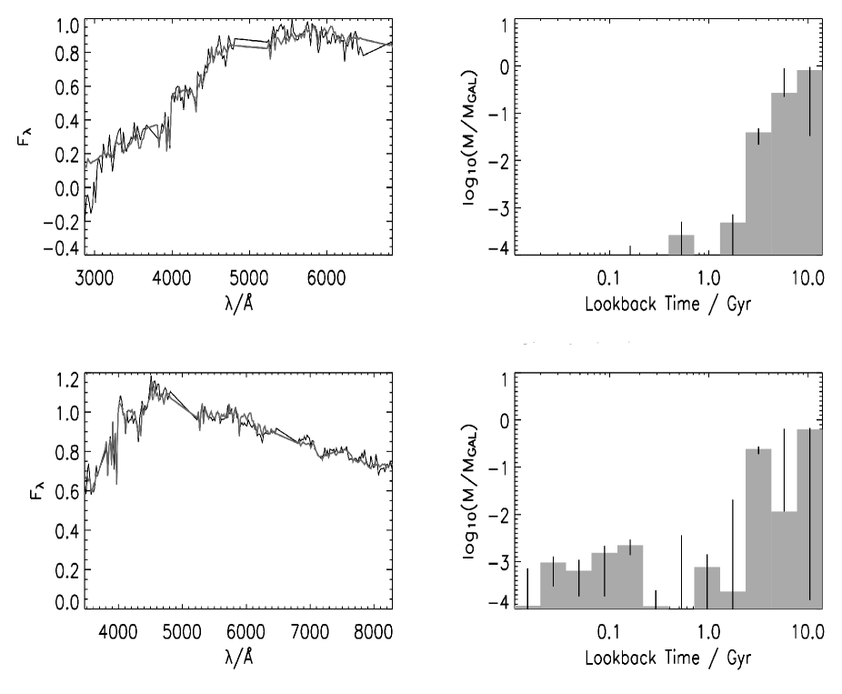
Figure 1: Two examples of spectra with the best-fitting model found by MOPED (left panels). The right-hand panels show the recovered star formation history, along with marginal errors determined by the MCMC method (see Appendix for details). Three areas have been removed to avoid contamination of the fitted spectrum by emission lines, at wavelengths around 3800, 5000 and 6600 angstroms. These regions are ignored in the fitting. The SDSS identifications of the galaxies are shown above the figures.

Star formation in galaxies takes place in giant molecular clouds that are relatively short-lived (about $10^{7}$ yr or less) during the whole life of the galaxy. It is therefore clear that star formation can be described in a rather model independent way by dividing time into widths of $10^{7}$ yr, each of which has a given metallicity. Then for a galaxy today whose star formation extends over most of the age of the universe, the problem amounts to determining $\approx 10^{3}$ parameters. This is firstly not tractable with current computing power and furthermore, as we will demonstrate below, the observed spectra of current galaxies may not have sensitivity to all episodes of star formation. Thus we adopt a different strategy which consists on a coarser grid than above. The bins in (lookback) time are chosen to have equal width in logarithmic space (this is discussed in detail in Reichardt, Jimenez & Heavens (2001)). With logarithmic lookback times, the error in the final spectrum caused by the uncertainty of the exact time at which star formation in the bin occured is roughly independent of time. The large bin widths at early times simply reflect the fact that there is little sensitivity in the final spectrum to the exact time that star formation takes place.

In the section below we will show that star formation histories and metallicities can be recovered with sensible errors if the grid contains 12 bins. The age bins start at a lookback time of 0.01, increasing in equal logarithmic steps with a spacing of 0.258. To each of these bins we assign two numbers, the fraction of the total stellar mass created in that time bin and the metallicity of the gas which formed that mass. Dust is modeled in a simple way by use of the Calzetti (1997) colour excess parameter, E(B-V), sufficient to describe the major effect of dust absorption on the integrated light of galaxies. The Calzetti model depends only on one parameter: the amount of dust in the galaxy. It is obvious that more sophisticated models are needed to describe the effect of dust in galaxies and this will be explored in a future paper. The model effectivly tilts the spectrum by supressing the blue end. The set of simple stellar population models used in this paper is the one by Jimenez et al. (1998, 2003), and we refer the reader to those references for a thorough discussion of the validity of the models (see also Jimenez, Flynn & Kotoneva (1998); Kotoneva, Flynn & Jimenez (2002)). Line emission from the galaxies has been removed, as the stellar spectral synthesis models do not include emission lines from gaseous regions, and the relationship between the emission line strengths and star formation history is less certain than the modeling of stellar features. A technicality is that the rest-frame wavelength coverage of the galaxies obviously depends on the redshift of the galaxy, so we make a one-off computation of a different set of MOPED vectors ${\bf b}_{m}$ for each of 49 values of redshift between $z=0$ and $0.34$. Extending the redshift range requires further MOPED vectors to be computed, and there are very few galaxies beyond $z=0.34$.

For reference, the fiducial model has star formation which increases linearly for increasing bin age, as well as the metallicity. The dust parameter is 0.02. The noise is assumed to be uncorrelated, and each wavelength bin considered is assumed to have the same error. This is not a bad approximation for the Sloan galaxies, after emission lines have been removed. The level of the noise simply scales the MOPED vectors, and we use the appropriate average error for each galaxy. We emphasize though that the precise choice of fiducial model and covariance matrix is not crucial and does not bias the parameter estimation, nor does a poor choice lead to significantly worse errors.

4 SDSS, and computational details

The SDSS includes $\sim 2$Å spectroscopy and $u,g,r,i$ and $z$ photometry, and will eventually contain $\sim$700,000 objects. We have analysed 37,752 galaxies from the Early Data Release (Stoughton et al., 2002), after removing objects not classified as galaxies or outside our redshift range. Details of the survey can be found in Gunn et al. (1998); York et al. (2000); Strauss et al. (2002). The spectra were binned to 20Å resolution, to match the models. Examples are shown in Fig.1.

It is not a trivial task to determine the best-fitting parameters, as the problem shows certain near-degeneracies (the well-known age-metallicity degeneracy being one), and the parameter space to be searched is large (25-dimensional). In addition, no guaranteed method exists to find a global maximum of the likelihood surface. We use a two-stage process for this task. First, a conjugate gradient method is used, with 50 random starting points, to reduce the chance of finding only local maxima which are not the global maximum. Second, the MCMC method is used to find the shape of the likelihood surface and determine errors; details are given in the Appendix. Finding formal errors is not a trivial task, for two reasons. Firstly, the reduced $\chi^{2}$ values of the best fits are formally too large (typically around six), which reflects the fact that spectrophotometric modelling in not perfect. In this case, the standard method of error determination (eg. Press et al. 1992) fails. The second problem is that, for noisy spectra (see fig. 1) degeneracies do remain, and it is difficult to quote errors for a multi-peaked likelihood surface. We assign errors by allowing $\Delta\chi^{2}$(full)=number of parameters. This procedure generally characterises the width of the highest peak in the likelihood surface.

The MCMC stage in some cases will find a better maximum likelihood solution, and this is then used for the parameter estimates. Typically, the conjugate gradient stage takes 40 seconds per galaxy, and the MCMC stage, with 300,000 evaluations, about 3 minutes per galaxy, on a 1.6 GHz Athlon PC workstation. Fig.1 shows the recovered star formation fractions and corresponding metallicities in the 12 lookback time periods for four galaxies. Note that the scale is logarithmic, and note that the mass of stars created in each time bin is normalised to the total mass of the best-fitting model. Thus the error bars can extend above a fraction of unity. We see that the star formation fractions are determined reasonably accurately where there is a significant contribution, but inevitably poorly determined otherwise. 12 bins is about the maximum number justified by the data; covariances between the estimates of the star formation in adjacent bins are beginning to appear. This is supported by information-theoretic studies of SDSS galaxy spectra which indicate $\sim 20$ independent components (J. Riden, private communication). This can be appreciated in the third panel from the top. There is a strong covariance between the estimates in the last two bins. However, this is for a galaxy with a very noisy spectrum. If the spectrum has got a higher signal to noise, as in the top panel, the covariance decreases.

Although Fig. 1 only shows two examples, they are representative of general trends in our analysis. The top galaxy shows a relatively old stellar population, with little star formation in the last Gyr. The lower galaxy shows a galaxy with evidence of a higher level of more recent star formation. Some remaining degeneracy is apparent in the results, especially in the oldest two bins, where some trade-off between the two is allowed. For the lower galaxy, although the formal best fit puts almost all of the old stars in the oldest bin, the error bars indicate that there are solutions which are almost as good which transfer much of that star formation into the 6Gyr old bin. Population boxes for the whole sample studied here will be freely available through http://www.roe.ac.uk in due course.

5 Results

5.1 Global star formation history of galaxies

By recovering the star formation and metallicity history of so many galaxies, we are able to derive the global histories. The assumption which we make here is that galaxies which are not selected for the SDSS have, on average, the same historical properties as the average of those which are. It is clear, though, that at high-redshift we are preferentially selecting bright galaxies, compared to low redshift (SDSS is a magnitude-limited survey).

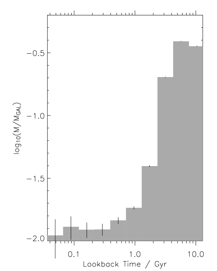
Figure 2: The average mass fraction of gas converted into stars as a function of time and lookback time. This figure is weighted by number.

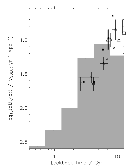
Figure 3: The rate of conversion of gas to stars, plotted against lookback time; results are weighted by the stellar mass. The symbols indicate previous measurements: diamonds are from Lilly et al. (1996), triangles from Connolly et al. (1997), squares from Steidel et al. (1999) and the cross from Tresse & Maddox (1998). All points have been dust corrected using the Steidel et al. (1999) correction factor.

The first quantity of interest is the mass fraction of gas converted into stars as a function of redshift. This is shown in Fig. 2. Star formation fractions have been determined for each galaxy as a function of rest-frame galaxy lookback time. The measurements are then assigned to lookback time relative to the present day by rebinning. We see that about 1/3 of the star formation in the SDSS galaxies occurs in the last 4 Gyr, and another 1/3 was formed more than 8 Gyr ago. The quality of the SDSS spectra does not seem to allow a finer time binning for old ages than the one presented here (see covariances between bins in Fig. 1), so it is difficult to estimate how many were formed at a really high redshift. Using currently-favoured cosmological parameters (flat universe, $\Omega_{m}=0.3$, $H_{0}=72$ km s^-1 Mpc^-1), a lookback time of 8 Gyr corresponds only to $z\sim 1$. It is clear that moderately higher signal to noise spectra would provide with the possibility of a finer grid of the oldest bin and thus a more accurate determination of the rate at which gas is converted into stars at high redshift. However, the recent bins (ages smaller than 4 Gyr, or equivalently $z<0.4$) are well resolved. It is interesting that 30% is also the fraction of stars presently in spheroids, which contain the oldest stellar populations, thus we could infer that most stars in spheroids were formed more than $8$ Gyr ago.

A quantity of great interest for the past few years has been the volume-average star formation rate in the universe as a function of redshift (e.g. Lilly et al. (1996); Madau et al. (1996); Hughes et al. (1998); Steidel et al. (1999)). This is derived by determining the current star formation rate from star-forming galaxies at different redshifts. Fig. 3 shows our findings from the SDSS fossil record evidence. As is apparent from the figure, we find a similar sharp decline in star formation rate with time, but we are able to extend the star formation histories to much more recent times, and we see that the trend continues at least to lookback times of 0.5 Gyr, representing a drop by a factor of 30 or more. The formal errors suggest a real increase in star formation at early times, but we caution against overinterpretation here in view of degeneracies in the last two bins which are apparent in fig. 1. Further, we have assumed that galaxies below the magnitude limit of the SDSS have the same star formation rate. Although, in the bins of fig. 3 we only plot the statistical errorsfrom the MOPED fitting, we estimate that other systematic errors (small number of galaxies and the exact number of galaxies per $Mpc^{3}$) contribute about 30% to the error in the height of each bin. The overplotted points are some recent measurements of the current star formation rate of galaxies from different surveys using the compilation in Steidel et al. (1999). Specifically, diamonds are from Lilly et al. (1996), triangles from Connolly et al. (1997) and squares from Steidel et al. (1999). All points have been dust corrected using the Steidel et al. (1999) correction factor. In addition we also plotted (cross) the measurement at $z\sim 0.2$ by Tresse & Maddox (1998).

The overall shape of the SFR as recovered from the SDSS is in reasonably good agreement with the instantaneous SFR estimates. We do find that the oldest bin is slightly below the penultimate one indicating a star formation rate of about 35% lower at early times than at the peak. However, we have found that these last two bins often show degeneracies in individual spectra, so the turndown at early times may not be significant. We also find that the decline in star formation continues to small lookback times.

5.2 Metallicity evolution with redshift

Figure 4: The average value of the metallicity for the 37,752 galaxies studied in this paper (horizontal bars). Also shown are stars from the Milky Way, and their averages (small and large diamonds) and the predictions of a closed-box model (solid line).

Figure 5: The evolution of the average total mass (solid), stellar mass (dashed) and gas mass (dotted), normalised to the final stellar mass, for an infall model constrained to give the right star formation and metallicity histories.

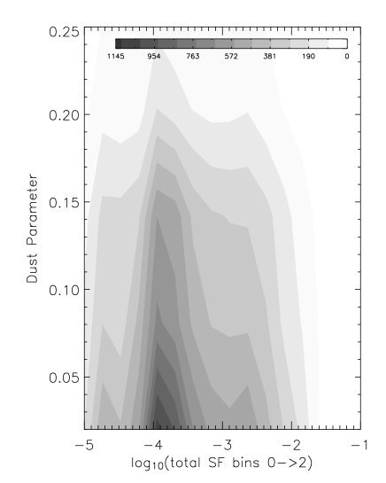
Figure 6: The joint distribution of dust content and recent (last 40 Myr) star formation rate in the SDSS sample. The number of galaxies in each contour level is shown in the upper bar.

We also compute the average metallicity of the gas which turns into stars at each epoch. This is shown in Fig.4, and shows some striking features. At high redshift the average metallicity increases with time, but then shows a systematic decrease, providing strong support for infall of relatively unprocessed gas into galaxies at lookback times between 4 and 0.1 Gyr. The average metallicity peaks at values of about solar. While stars formed more than 8 Gyr ago and less than 2 Gyr have metallicities slightly lower, about half solar. The rise in metallicity from early times to age $\sim 3$ Gyr can be accounted for by closed-box models, but not the strong decline in metallicity at lookback times of less than 3 Gyr: the solid line shows the predictions of the closed-box model (e.g. Binney & Merrifield (1998))

$$Z(t)=-p\,ln\left[\frac{M_{g}(t)}{M_{g}(0)}\right]$$ (4)

where p is the yield, $M_{g}(t)$ the mass in gas at time $t$ and $M_{g}(0)$ the initial gas mass. Note that for ages below $3$ Gyr, the closed-box model is inconsistent with the data. The line has $p=0.02$ and $M_{g}(0)=1$ (in units of the final stellar mass), but it is obvious that no closed-box model can account for the decline of metallicity.

The diamond symbols correspond to ages and metallicities from the Edvardsson et al. (1993) sample of stars in the Milky Way with accurate ages and metallicities. The large diamonds average these data. Although the SDSS galaxies include spheroids and not only disk systems, it is gratifying that the overall shape and range of $Z(t)$ is similar to that for Milky Way stars, although the Milky Way is apparently offset to later times when compared with the SDSS population.

Fig. 5 shows the results from an accretion-box or infall model (e.g. Binney & Merrifield (1998)), where we allow for fresh infall of gas constrained to reproduce the star formation and metallicity history. The total mass (stars plus gas) $M_{t}$ then obeys the following equation

$$\delta M_{t}={p\over Z}\delta M_{s}-(M_{t}-M_{s}){\delta Z\over Z}.$$ (5)

The figure assumes $p=0.02$ and $M_{g}(0)=1$ (normalised to the final stellar mass), but the general features of the curve are robust, with fresh infall clearly necessary to reduce the metallicity. The different lines correspond to the evolution of the average total mass (solid), stellar mass (dashed) and gas mass (dotted), normalised to the final stellar mass, for an infall model constrained to give the right star formation and metallicity histories. Note the significant amount of gas supply in the last 3 Gyr. With these yield and initial gas mass, outflow is formally required in the last Gyr.

5.3 Dust content

In Fig. 6 we show the joint distribution of dust content and star formation fraction in the last 40 Myr. There is no strong evidence of a trend of higher dust content with higher recent star formation, in contrast to the findings of Kauffmann et al. (2002).

6 Discussion and Conclusions

We have determined the past star formation history of the Universe from the present-day fossil record of the spectra of more-or-less present-day galaxies, and made comparisons with previous alternative methods based on computing the essentially instantaneous star formation rate from samples over a range of redshifts. We have presented a MOPED analysis of 37,752 galaxy spectra from the SDSS Early Data Release. MOPED allows very rapid determination of the star formation and metallicity history of each galaxy, through carefully-designed and optimised data compression. We have therefore been able to dispense with the usual oversimplifying assumptions which are usually employed to make this sort of problem tractable, such as exponentially-decaying star formation rates, bursts and so on. We recover the star formation fraction and the metallicity in 12 equal size bins of log(lookback time), plus one parameter describing the dust content, using the Calzetti (1997) model.

Previous studies of the star formation history of galaxies have generally used measurements of the contemporary star formation rates, and the history has been constructed by making observations at a range of redshifts. These studies have indicated a decline in the star formation rate to the present-day. This behaviour should be apparent in the fossil record of the spectrum of galaxies at low redshift. In this paper one of our main conclusions is that this evidence is present in the Sloan Digital Sky Survey Early Data Release sample: the average star formation rate in the SDSS sample has been in decline for the last $\sim 6$ Gyr or so, at which point there is some evidence for a peak in the star formation rate. We find that the subsequent decline has contintued to very recent lookback times ($<0.5$ Gyr).

On average, each galaxy produced about 30% of the stars more than $\sim 8$ Gyr ago. This corresponds to all stars in spheroids being formed at $z>1$. This age distribution is consistent with the age distribution of stars in the Milky Way. 65% of galaxies have some star formation older than 8 Gyr, and 97% have some star formation older than 2 Gyr.

In addition, we find that the average metallicity of the gas rises with time to a peak $\sim 3$ Gyr ago, and has been in significant decline since then. This is clearly in contradiction with closed-box chemical evolution models, but can be accounted for with infall models (e.g. Binney & Merrifield (1998)). The maximum average metallicity is about solar, for stars formed 2-8 Gyr ago. Stars formed recently, $<1$ Gyr ago, in SDSS galaxies have metallicities as low as $\sim 0.5Z_{\odot}$ on average, similar to that of stars in SDSS galaxies formed more than 8 Gyr ago. We also find a very weak correlation between the dust content of a galaxy and its recent star formation rate.

We can compare our analysis and results with the studies of Kauffmann et al. (2002). That paper used the 4000Å break, the $H\delta$ feature, and four broad-band measurements. Thus each galaxy spectrum was compressed into six numbers, chosen on the basis of knowledge of the evolution of stellar spectral features and model evolution of broad-band colours. MOPED’s approach is rather different; firstly it uses the entire spectrum, and uses model predictions to find which wavelengths are most sensitive to the parameters of interest. It then does an automatic data compression step, reducing the spectrum to (in this paper) 25 linear combinations which retain as much information as possible. In this way, we are able to get results which are in principle as accurate as the modelling allows. Furthermore, the speed advantage offered by the data compression step allows us to be ambitious in what we extract: we are able to estimate star formation fractions in twelve time bins, plus twelve associated metallicities of the star-forming gas, and a dust parameter. Without the radical data compression, the searching of this 25-dimensional space would be prohibitively slow, and we would be restricted to simple parametrisations of the star formation history, as has been done historically.

Population boxes for the whole sample studied here will be released through http://www.roe.ac.uk in due course.

Appendix: Error estimation through Monte Carlo Markov-Chain algorithms

Given that the number of parameters will be usually large (typically more than 10 and in this case 25), computation of a grid to explore the likelihood surface is impractical – simply using 10 grid points per dimension would require $10^{25}$ evaluations. An alternative approach is to use the Fisher matrix around the maximum of the likelihood to compute errors. Although this is a fast and efficient method, it assumes that the likelihood surface is a multivariate gaussian which may not be the case in general.

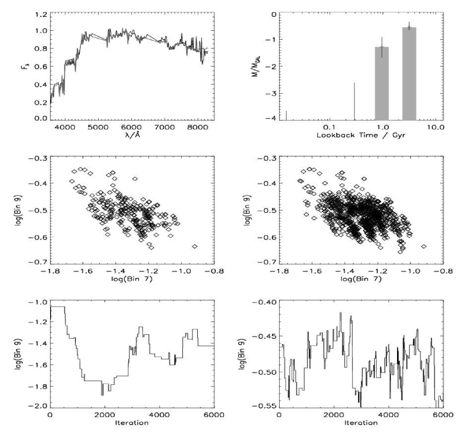
Figure 7: Some details of the application of MOPED to an individual SDSS galaxy. The top left panel shows the galaxy spectrum (black) and the best fit Jimenez model (grey). The corresponding star formation fractions are shown in the top right panel. The middle panels show the MCMC points with highest likelihood values, in projection onto parameter plane 7 and 9, which are the bins showing significant star formation, for chains of 30,000 (left) and 300,000 (right). The lower panels show the effects of different step sizes on the estimation of parameter 9. The convergence of the parameter estimates shown in the lower part of the figure is discussed in the appendix.

In the general case, an efficient method to sample the likelihood surface is through the Markov Chain Monte Carlo (MCMC) algorithm (Metropolis et al., 1953; Hastings, 1970). In essence the Markov chain algorithm is very simple: a chain of likelihood values in the parameter space is created in the following way. At each point, a random step is made in parameter space, and a random number between 0 and 1 is drawn. This number is essentially compared with the ratio of the likelihood values between the current step and the previous one, although there are some slight modifications, especially near the boundaries of the parameter space. If the value of the likelihood ratio is bigger than 1 or the random number, then the current step is accepted and added to the chain. If, however, it is smaller than the random number, then the point is rejected and not added to the chain. Asymptotically, the distribution of points in the chain samples the likelihood surface in an unbiased way.

In this paper, we use a uniform prior within certain bounds to produce the step. If knowledge about the shape of the surface is known a priori, then the random stepping can be done more efficiently by using this a priori information. The Fisher matrix can sometimes be useful for this, but if the topology of the likelihood hyper-surface is not known, it may be inaccurate. Marginal errors are then trivial to compute by looking at the distribution of all points for a single parameter. The method is very fast and efficient but the challenge is to adjust the step size of the jump so the likelihood surface around the maximum is explored with the minimum number of steps.

There are some rules to decide the size of the jump a priori (see Gilks et al. (1996)), we find that the most efficient time step can be found by exploration of a few thousand chains for a few galaxy spectra.

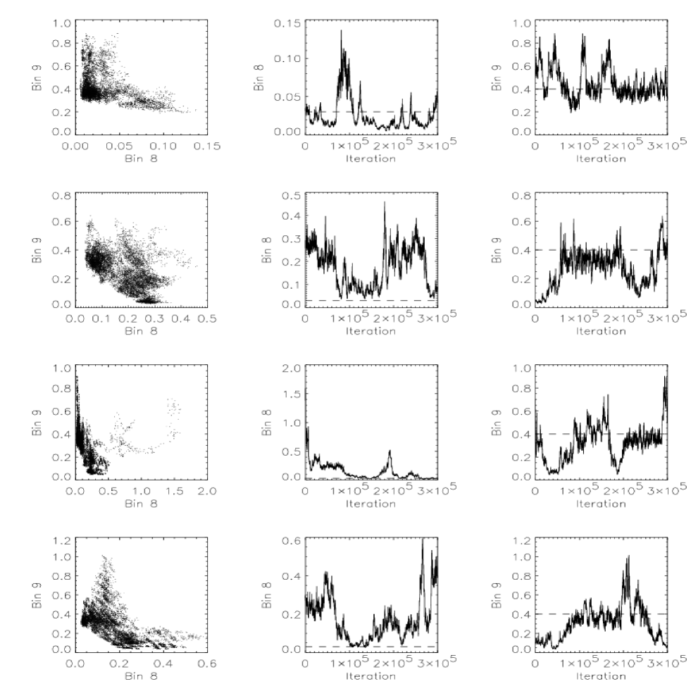
Figure 8: Convergence test for MCMC. Four chains of length 300,000 steps have been started at different points in parameter space for the galaxy shown in Fig. 7. The far left panel shows the values of the star formation in bins 8 and 9 for each chain. In order to show how the chain samples the likelihood surface, the middle left panel shows those points in the chain within a reduced $\Delta\chi^{2}=1$ of the best-fitting solution. The right-hand panels show the values of the star formation parameters explored by the chains. Note that the excursion to the right in the third row is in fact the starting point of the chain. The long-dashed horizontal lines show the best-fitting solution.

As an example of Markov-chain convergence examine Fig. 7. The top-left panel shows a typical spectrum of a galaxy with an old stellar population. The top-right panel displays the recovered star formation history with errors computed using the MCMC. The middle-left panel shows the distribution of points in the plane of parameter values recovered from the MCMC for only 30,000 points in the chain, showing only those within reduced $\Delta\chi^{2}=1$ of the minimum $\chi^{2}$ point. The middle-right panel shows the same but this time for a chain with 300,000 points. The chain with a small number of points shows a rugged pattern, with a few unexplored areas, but the chain with 300,000 points has covered the region of the likelihood space that is most favoured quite well. More specifically, it is clear that the chain with a small number of points has not come back to the starting point of the chain a few times. This feature is required to establish convergence, and the left hand chain is said to be not well mixed, although in this case it provides a good estimate of the errors. On the contrary, the right hand chain with a small step has oscillated a few times around the starting point.

In the above chains the time step was chosen by trial and error. In principle, the step size can be chosen optimally a priori. For one parameter, for example, the step size should be such that the rejection rate of points is about 60%, leading to a non-negligible chance of the chain exploring regions in the likelihood surface that are more than 3$\sigma$ away from the best solution. Obviously, for more parameters the rejection rate will decrease significantly, since there are many more ways the jump can explore an unlikely region of the parameter space. High acceptance rates are indicative of too small a jump step (see below).

The two bottom panels of figure 7 show the values of one parameter (star formation for the bin with most star formation) for part of two chains. The left-bottom panel shows a chain with a step that is too big. Note how the chain remains at same value of the parameter for many steps. The path of the parameter value for the change shows a clear “staircase” pattern, and the chain is inefficient. On the other hand, the right-bottom panel shows a chain with a much better step size. In this case the chain does not dwell for long on a single value of the parameter.

Our experiments show that significant improvements in chain convergence can be obtained by using a nonuniform jump size. The star formation history is divided into two sections, the first covering mass fractions from $10^{-7}$ (essentially zero) to $10^{-4}$, the second from $10^{-4}$ to 10. In the first region we have 100 logarithmically-spaced points, in the second a thousand. The maximum jump we allow is 20 steps. Similarly, there are 64 values of metallicity in a grid, log spaced between $0.01<Z/Z_{\odot}<5$ and the optimal jump size is 5 grid points. Dust is computed on a linear grid, with 64 elements, between 0.02 and 1.28 and optimal jump size of 3 grid elements. The chain is well mixed for 300,000 steps and the acceptance rate is typically about 2% in 25 dimensions.

A more robust way to estimate the convergence of the chain is the following: start 4 or more chains from widely-separated points in the parameter space and check when the variance for all parameters within the chain and between chains are indistinguishable; at this point the chains have converged. The point is well illustrated in Fig. 8. The left four panels show the distribution of points in a projection of the likelihood hyper-surface for two adjacent bins for a random galaxy with only significant star formation in bins 8 and 9. The second column of panels shows only those points for which reduced $\Delta\chi^{2}<1$ from the best value in the likelihood, while the 1 column of panels shows all 300,000 points in the chains. In the right panels we show the values of bins 8 and 9 for the four chains and 300000 jumps. The dashed line is the best-fitting value for the parameter. A few features become apparent by visual inspection. When the chains start from values different from the best fit, it takes 50-100,000 steps for them to converge. After this, the chain remains on the good valley solution for some time, before undergoing a random excursion away from the best solution, before returning at some point. This returning behaviour is required for convergence.

If we use the above convergence criterion, we see that chains converge at different points in path. For example, the chain on the top panel for bin 9 only converges after 200,000 points. While the second chain from the top, does so after only 50,000 steps for bin 9. This illustrates how important it is to run chains for a long enough time and estimate convergence.

An alternative approach is to run only one chain from one point in the parameter space and let it run for long enough as to explore most of the likelihood space. A good test to check convergence then is to monitor the likelihood values as a function of the step. The chain should return to close to the maximum likelihood solution. In the present paper we follow this criterion and in all cases we find chains have converged after 300,000 steps, as illustrated in the example of Fig. 8.

It is worth emphasizing that the chain needs to be able to explore the likelihood hyper-surface well in the vicinity of the peak in order to be sure errors are derived properly. Also, there is some danger in using local approximations to the likelihood surface (the Fisher matrix) to compute the length of each jump. Imagine, a flat valley in the likelihood surface with a narrow region within where the likelihood is better. A first jump may bring you into the valley, then the Fisher matrix will indicate that the hyper-surface is locally very flat which will systematically provide a very large jump and therefore the better value will be systematically missed.

6.1 Covariances between bins

The left panels in Fig. 8 illustrate how covariances appear between adjacent bins. The far left panel shows the values of the whole chain, whereas the middle-left panel shows only those points within reduced $\Delta\chi^{2}=1$ of the best-fitting solution. Note how the paths for bin values follow a common pattern: star formation in one bin is traded by star formation on the adjacent bin (with different metallicity) - the sum of bins 8 and 9 is well constrained in this example. We also see from the right-hand panels that the chains spend longer periods close to the best-fitting parameter where the parameter has more star formation (parameter 9) than less (parameter 8).

References

- Baldry et al. (2002) Baldry et al. I. K., 2002, ApJ, 569, 582
- Binney & Merrifield (1998) Binney J., Merrifield M., 1998, Galactic astronomy. Princeton University Press, 1998.
- Blain et al. (2002) Blain A. W., Smail I., Ivison R., Kneib J.-P., Frayer D. T., 2002, Phys. Rept., 369, 111
- Calzetti (1997) Calzetti D., 1997, AJ, 113, 162
- Connolly et al. (1995) Connolly A., Szalay A., Bershady M., Kinney A., Calzetti D., 1995, AJ, 110, 1071
- Connolly et al. (1997) Connolly A. J., Szalay A. S., Dickinson M., Subbarao M. U., Brunner R. J., 1997, ApJ, 486, L11
- Edvardsson et al. (1993) Edvardsson B., Andersen J., Gustafsson B., Lambert D. L., Nissen P. E., Tomkin J., 1993, A&A, 275, 101
- Folkes et al. (1999) Folkes et al. 1999, MNRAS, 308, 459
- Francis et al. (1992) Francis P., Hewett P., Foltz C., Chaffee F., 1992, ApJ, 398, 476
- Gilks et al. (1996) Gilks W., Richardson S., Spiegelhalter D., 1996, Markov Chain Monte Carlo in Practice. Chapman and Hall
- Gunn et al. (1998) Gunn et al. J. E., 1998, AJ, 116, 3040
- Gupta & Heavens (2002) Gupta S., Heavens A. F., 2002, MNRAS, 334, 167
- Hastings (1970) Hastings W., 1970, Biometrika, 57, 97
- Heavens et al. (2000) Heavens A., Jimenez R., Lahav O., 2000, MNRAS, 317, 965
- Hughes et al. (1998) Hughes et al. D. H., 1998, Nature, 394, 241
- Jimenez et al. (2003) Jimenez R., Dunlop J., MacDonald J., Padoan P., Peacock J., 2003, in preparation
- Jimenez et al. (1998) Jimenez R., Flynn C., Kotoneva E., 1998, MNRAS, 299, 515
- Jimenez et al. (1998) Jimenez R., Padoan P., Matteucci F., Heavens A. F., 1998, MNRAS, 299, 123
- Kauffmann et al. (2002) Kauffmann et al. G., 2002, astro-ph/0205070
- Kotoneva et al. (2002) Kotoneva E., Flynn C., Jimenez R., 2002, MNRAS, 335, 1147
- Lilly et al. (1996) Lilly S. J., Le Fevre O., Hammer F., Crampton D., 1996, ApJ, 460, L1
- Madau et al. (1996) Madau P., Ferguson H. C., Dickinson M. E., Giavalisco M., Steidel C. C., Fruchter A., 1996, MNRAS, 283, 1388
- Madgwick et al. (2002) Madgwick D., Sommerville R., Lahav O., Ellis R., 2002, astro-ph/0210471
- Metropolis et al. (1953) Metropolis N., Rosenbluth A., Rosenbluth M., Teller M., Teller E., 1953, J. Chem. Phys., 21, 1087
- Murtagh & Heck (1987) Murtagh F., Heck A., 1987, Multivariate Data Analysis. Reidel, Dordrecht
- Press et al. (1992) Press W. H., Teukolsky S. A., Vetterling W. T., Flannery B. P., 1992, Numerical recipes in FORTRAN. The art of scientific computing. Cambridge: University Press, 1992, 2nd ed.
- Reichardt et al. (2001) Reichardt C., Jimenez R., Heavens A. F., 2001, MNRAS, 327, 849
- Ronen et al. (1999) Ronen R. T., Aragon-Salamanca A., Lahav O., 1999, MNRAS, 303, 284
- Slonim et al. (2000) Slonim N., Somerville R., Tishby N., Lahav O., 2000, astro-ph, 0005306
- Steidel et al. (1999) Steidel C. C., Adelberger K. L., Giavalisco M., Dickinson M., Pettini M., 1999, ApJ, 519, 1
- Stoughton et al. (2002) Stoughton et al. C., 2002, AJ, 123, 485
- Strauss et al. (2002) Strauss et al. M. A., 2002, AJ, 124, 1810
- Tegmark et al. (1997) Tegmark M., Taylor A., Heavens A., 1997, ApJ, 480, 22
- Tresse & Maddox (1998) Tresse L., Maddox S. J., 1998, ApJ, 495, 691
- Vergely et al. (2002) Vergely J.-L., Lancon A., Mouchine M., 2002, astro-ph/0209018
- York et al. (2000) York et al. D., 2000, AJ, 120, 1579