The State of the Dark Energy Equation of State

Abstract

By combining data from seven cosmic microwave background experiments (including the latest WMAP results) with large scale structure data, the Hubble parameter measurement from the Hubble Space Telescope and luminosity measurements of Type Ia supernovae we demonstrate the bounds on the dark energy equation of state $w_{Q}$ to be $-1.38<w_{Q}<-0.82$ at the $95\%$ confidence level. Although our limit on $w_{Q}$ is improved with respect to previous analyses, cosmological data does not rule out the possibility that the equation of state parameter $w_{Q}$ of the dark energy $Q$ is less than -1. We present a tracking model that ensures $w_{Q}\leq-1$ at recent times and discuss the observational consequences.

I Introduction.

There is now a growing body of evidence that the evolution of the universe may be dominated by a dark energy component $Q$, with present-day energy density fraction $\Omega_{Q}\simeq 2/3$ super1 . Although a true cosmological constant $\Lambda$ may be responsible for the data, it is also possible that a dynamical mechanism is at work. One candidate to explain the observations is a slowly-rolling dynamical scalar “quintessence” field Wetterich:fm -Caldwell:1997ii . Another possibility, known as “k-essence” Armendariz-Picon:1999rj -Chiba:1999ka , is a scalar field with non-canonical kinetic terms in the lagrangian. Dynamical dark energy models such as these, and others parker -bastero-mersini , have an equation of state, $w_{Q}\equiv p_{Q}/\rho_{Q}$ which varies with time compared to that of a cosmological constant which remains fixed at $w_{Q=\Lambda}=-1$. Thus, observationally distinguishing a time variation in the equation of state or finding $w_{Q}$ different from $-1$ will rule out a pure cosmological constant as an explanation for the data, but be consistent with a dynamical solution.

In the past years many analyses of several cosmological datasets have been produced in order to constrain $w_{Q}$ (see e.g. rachel and references therein). In these analyses the case of a constant-with-redshift $w_{Q}$, in the range $w_{Q}\geq-1$ was considered. The assumption of a constant $w_{Q}$ is based on several considerations: first of all, since both the luminosities and angular distances (that are the fundamental cosmological observables) depend on $w_{Q}$ through multiple integrals, they are not particularly sensitive to variations of $w_{Q}$ with redshift (see e.g. maor1 , rachel ). Therefore, with current data, no strong constraints can be placed on the redshift-dependence of $w_{Q}$. Second, for most of the dynamical models on the market, the assumption of a piecewise-constant equation of state is a good approximation for an unbiased determination of the effective equation of state (wang0 )

$$w_{\rm eff}\sim\frac{\int w_{Q}(a)\Omega_{Q}(a)da}{\int\Omega_{Q}(a)da}$$ (1)

predicted by the model. Hence, if the present data is compatible with a constant $w_{Q}=-1$, it may not be possible to discriminate between a cosmological constant and a dynamical dark energy model.

The limitation to $w_{Q}>-1$, on the contrary, is a theoretical consideration motivated, for example, by imposing on matter (for positive energy densities) the null energy condition, which states that $T_{\mu\nu}N^{\mu}N^{\nu}>0$ for all null 4-vectors $N^{\mu}$. Such energy conditions are often demanded in order to ensure stability of the theory. However, theoretical attempts to obtain $w_{Q}<-1$ have been considered Caldwell:1999ew ; Schulz:2001yx ; parker ; frampton ; Ahmed:2002mj while a careful analysis of their potential instabilities has been performed in CHT .

Moreover, Maor et al. maor2 have recently shown that one may construct a model with a specific z-dependent $w_{Q}(z)\geq-1$, in which the assumption of constant $w_{Q}$ in the analysis can lead to an estimated value $w_{\rm eff}<-1$. This further illustrates the necessity of extending dark energy analyses to values of $w_{Q}<-1$.

In this paper we combine constraints from a variety of observational data to determine the currently allowed range of values for the dark energy equation of state parameter $w_{Q}$. The data used here comes from six recent Cosmic Microwave Background (CMB) experiments, from the power spectrum of large scale structure (LSS) in the 2dF 100k galaxy redshift survey, from luminosity measurements of Type Ia supernovae (SN-Ia) super1 and from the Hubble Space Telescope (HST) measurements of the Hubble parameter.

Our analysis method and our datasets are very similar to the one used in a recent work by Hannestad and Mortsell (mortsell ). We will compare our results with those derived in this earlier paper in the conclusions.

In the next section, we demonstrate the plausibility of $w_{Q}<-1$ by presenting a class of theoretical models in which this result may be obtained explicitly. In our model the equation of state parameter is approximately piecewise constant and hence provides a specific example of a model which would fit the data described in the remainder of the paper. The methods used to obtain combined constraints on the dark energy equation of state are described in section III. Our likelihood analysis is presented in section IV and our summary and conclusions are given in section V.

II A Model with $w_{Q}<-1$.

It is a simple exercise to show that a conventional scalar field lagrangian density cannot yield an equation of state parameter $w_{Q}<-1$. There are, however, a number of ways in which the lagrangian can be modified to make $w_{Q}<-1$ possible. For example, one may reverse the sign of the kinetic terms, leading to interesting cosmological and particle physics behavior Caldwell:1999ew -CHT .

Let us motivate the study of $w_{Q}<-1$ cosmologies by describing a class of models, with positive kinetic energy, in which such evolution arises. The model we consider is very much in the spirit of k-essence Armendariz-Picon:2000dh ; Armendariz-Picon:2000ah . Comments on the similarities and differences between the two are briefly discussed at the end of this section.

Consider a theory of a real scalar field $\phi$, assumed to be homogeneous, with a non-canonical kinetic energy term. The lagrangian density is

$${\cal L}=f(\phi)g(X)-V(\phi)\ ,$$ (2)

where $f(\phi)$, $g(X)$ are positive semi-definite functions, $V(\phi)$ is a potential and $X\equiv{\dot{\phi}}^{2}/2$. The energy-momentum tensor for this field is straightforward to calculate and yields the usual perfect fluid form with pressure $p$ and energy density $\rho$ given by

$$p={\cal L}=f(\phi)g(X)-V(\phi)\ ,$$ (3)

$$\rho=\left[2X\frac{dg(X)}{dX}-g(X)\right]f(\phi)+V(\phi)\ .$$ (4)

Thus, defining $w_{\phi}\equiv p/\rho$ one obtains

$$w_{\phi}=\frac{g(X)f(\phi)-V(\phi)}{\left[2X\frac{dg(X)}{dX}-g(X)\right]f(\phi)+V(\phi)}\ .$$ (5)

If the lagrangian (2) is to yield $w_{\phi}<-1$ then (5) implies

$$g^{\prime}(X)<0\ ,$$ (6)

where $g^{\prime}(X)\equiv dg(X)/dX$ and we have used $f(\phi)\geq 0$ and $X\geq 0$. We therefore require that $g(X)$ be a strictly monotonically decreasing function. It is interesting to note in passing that, provided $f(\phi)$ is positive semi-definite, the functional forms of $f(\phi)$ and $V(\phi)$ play no role in determining whether $w_{\phi}$ is less than or greater than -1.

However, a constraint involving the potential does arise from the requirement that the energy density of the theory satisfy $\rho>0$. This yields

$$g(X)-2Xg^{\prime}(X)<\frac{V(\phi)}{f(\phi)}\ .$$ (7)

A necessary condition that the theory be stable is that the speed of sound of $\phi$ be positive Garriga:1999vw (see CHT for a detailed stability analysis of models with $w_{Q}<-1$). This yields

$$c_{s}^{2}\equiv\frac{\partial p}{\partial\rho}=\frac{p_{,X}}{\rho_{,X}}=\frac{g^{\prime}(X)}{g^{\prime}(X)+2Xg^{\prime\prime}(X)}>0\ ,$$ (8)

where a subscript $,X$ denotes a partial derivative with respect to $X$. Since we have already specified $g^{\prime}(X)<0$ this may be written as

$$g^{\prime\prime}(X)<-\frac{g^{\prime}(X)}{2X}$$ (9)

Notice the difference between this class of models and the k-essence family in terms of the potential $V(\phi)$ and the constraints placed on the functions $g(X)$ and $f(\phi)$.

Let us illustrate these constraints with a simple example $g(X)=e^{-\alpha X}$, with $\alpha>0$. This function trivially satisfies the constraints (6),(9). The constraint (7) then yields

$$\frac{V(\phi)}{f(\phi)}>(2\alpha X+1)e^{-\alpha X}\ .$$ (10)

In the asymptotic regions this becomes $V/f>0$ as $X\rightarrow\infty$ and $V/f>1$ as $X\rightarrow 0$. This may be satisfied without a particularly large potential by arranging an appropriately behaved $f(\phi)$, since (7) constrains only the ratio $V/f$, making fine-tuning issues less severe.

Let us now assume a (flat) Friedmann, Robertson-Walker (FRW) ansatz for the space-time metric

$$ds^{2}=-dt^{2}+a(t)^{2}d\overrightarrow{x}^{2}\ ,$$ (11)

with $a(t)$ the scale factor. The resulting Einstein equations then become the Friedmann equation

$$H^{2}\equiv\left(\frac{{\dot{a}}}{a}\right)^{2}=\frac{8\pi G}{3}\rho$$ (12)

and the acceleration equation

$$\frac{{\ddot{a}}}{a}=-\frac{4\pi G}{3}(\rho+3p)\ .$$ (13)

One then solves these equations along with those for the scalar field. In the case of k-essence with $w_{Q}>-1$ it has been shown Armendariz-Picon:1999rj -Armendariz-Picon:2000ah that tracking behavior can be obtained. This means that for a wide range of initial conditions, the energy density of the field $\phi$ naturally evolves so as to track the energy density in matter, providing some insight into why dark energy domination began only recently in cosmic history. In our model, in which we have included a potential for $\phi$ and are in the regime $w_{Q}<-1$, the analysis becomes somewhat more involved. Nevertheless, it can be shown that tracking behavior persists. However, as in all rolling scalar models, some fine-tuning remains, since one must ensure the right amount of dark energy density today.

III Comparison with Observations: Method

We restrict our analysis to flat models, for which the effects of dark energy with $w_{Q}\geq-1$ on the angular power spectrum of the CMB anisotropies have been carefully analyzed (see e.g. rachel and references therein). The main effect of changing the value of $w_{Q}$ on the CMB anisotropies is to introduce a shift by a linear factor ${\cal R}$ in the $l$-space positions of the acoustic peaks in the angular power spectrum Bond:1997wr . This shift is given by

$${\cal R}=\sqrt{(1-\Omega_{Q})}y\ ,$$ (14)

where

$$y=\int_{0}^{z_{dec}}\frac{dz}{\sqrt{(1-\Omega_{Q})(1+z)^{3}+\Omega_{Q}(1+z)^{3(1+w_{Q})}}}\ .$$ (15)

In order to illustrate this effect, we plot in Figure 1 a set of theoretical power spectra, computed assuming a standard cosmological model with the relative density in cold dark matter $\Omega_{cdm}h^{2}=0.12$, that in baryons $\Omega_{b}h^{2}=0.022$, with Hubble parameter $h=0.69$ but with $w_{Q}$ varied in the range $(-4,-0.5)$. It is clear that decreasing $w_{Q}$ shifts the power spectrum towards smaller angular scales $\theta\sim l^{-1}$.

In considering the CMB power spectrum, it is important to note that there is some degeneracy among the possible choices of cosmological parameters. First of all, the shift produced by a change in $w_{Q}$ can easily be compensated by a change in the curvature. However, degeneracies still exist even when we restrict to flat models. To emphasize this we plot in Figure 2 some degenerate spectra, obtained by keeping $\Omega_{b}h^{2}$, $\Omega_{M}h^{2}$, and ${\cal R}$ fixed, in a flat universe. In practice, in order to preserve the shape of the spectrum while decreasing $w_{Q}$, one has to increase $\Omega_{Q}$. For flat models, one must therefore decrease $\Omega_{M}$ and, since $\Omega_{M}h^{2}$ must be constant, increase $h$. Therefore, even if the CMB spectra are degenerate, combining the CMB information with priors on $\Omega_{M}$ and $h$ can be extremely helpful in bounding $w_{Q}$.

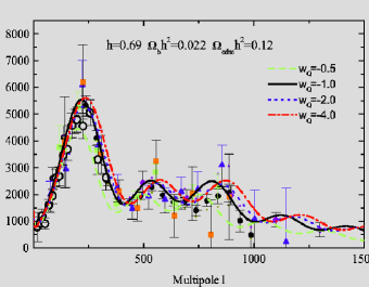
Figure 1: The effect of varying $w_{Q}$ on the COBE-normalized CMB angular power spectrum and present CMB data. Since the shift of the power spectrum is proportional to ${\cal R}\ell$, the discrepancy is more important for higher values of $\ell$.

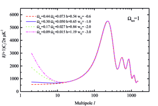
Figure 2: Degenerate CMB power spectra The models are computed assuming flatness ($\Omega_{tot}=\Omega_{M}+\Omega_{Q}=1$). On large angular scales the Integrated Sachs Wolfe effect breaks the degeneracy for highly negative values of $w_{Q}$. In general, the degeneracy of the spectra can be broken with a strong prior on $h$ or on $\Omega_{M}$.

On large angular scales the time-varying Newtonian potential after decoupling generates CMB anisotropies through the Integrated Sachs-Wolfe (ISW) effect. This is clearly seen in Figure 2 and is more pronounced for more negative values of $w_{Q}$. The effect depends not only on the value of $w_{Q}$ but also on its variation with redshift. However, this is difficult to disentangle from other cosmological effects.

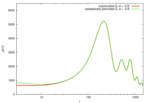
Figure 3: Effect of including perturbations in the dark energy fluid with a constant equation of state in the CMB power spectrum. Since dark energy dominates at late redshifts, the effect is present only on large angular scales.

In all our analysis we will neglect perturbations in the dark energy component. The reasons for this simplification are twofold: on the one hand we prefer our analysis to remain as model-independent as possible, so that the results obtained here are not affected by the choice of a particular dark energy model. The study of the perturbations in particular quintessential models goes beyond the scope of this paper. On the other hand, this approximation is also satisfied in a broad class of models and it is not completely straightforward to conclude that the inclusions of perturbations, while consistent with General Relativity, would yield a better approximation for a particular model of dark energy. As an example, in Figure 3, we plot the CMB power spectra for $w=-0.8$ computed with and without assuming adiabatic perturbations in the dark energy fluid as in saralewis . As we can see, since dark energy dominates the overall density only well after recombination, the major effects are only on very large scales. We found that the inclusion of perturbations has no relevant effect on our results for models with $w>-1$ where the computations of the perturbations are meaningful.

In order to bound $w_{Q}$, we consider a template of flat, adiabatic, $Q$-CDM models computed with CMBFAST sz . We sample the relevant parameters as follows: $\Omega_{cdm}h^{2}=0.01,...0.40$, in steps of $0.01$; $\Omega_{b}h^{2}=0.001,...,0.040$, in steps of $0.001$, $\Omega_{Q}=0.0,...,0.95$, in steps of $0.05$ and $w_{Q}=-3.0,...,-0.4$ in steps of $0.05$. Note that, once we have fixed these parameters, the value of the Hubble constant is not an independent parameter, since it is determined through the flatness condition. We adopt the conservative top-hat bound $0.45<h<0.85$.

We allow for a reionization of the intergalactic medium by varying the Compton optical depth parameter $\tau_{c}$ over the range $\tau_{c}=0.05,...,0.40$ in steps of $0.05$.

For the CMB data we use the recent temperature and cross polarization results from the WMAP satellite (Bennett:2003bz ) using the method explained in (Verde:2003ey ) and the publicly available code on the LAMBDA web site. We further include the results from the BOOMERanG-98 ruhl , DASI halverson , MAXIMA-1 lee , CBI pearson , VSAE grainge , and Archeops benoit experiments by using the publicly available correlation matrices and window functions. We consider $7\%$, $10\%$, $4\%$, $5\%$, $3.5\%$ and $5\%$ Gaussian distributed calibration errors for the Archeops, BOOMERanG-98, DASI, MAXIMA-1, VSA, and CBI experiments respectively and include the beam uncertainties using the analytical marginalization method presented in bridle . The likelihood ${\cal L}$ for a given theoretical model is defined by

$$-2\ln{\cal L}=(C_{B}^{th}-C_{B}^{ex})M_{BB^{\prime}}(C_{B^{\prime}}^{th}-C_{B^{\prime}}^{ex})\ ,$$ (16)

where $M_{BB^{\prime}}$ is the Gaussian curvature of the likelihood matrix at the peak and $C_{B}$ is the theoreical/experimental signal in the bin (BJK ).

In addition to the CMB data we also consider the real-space power spectrum of galaxies in the 2dF $100$k galaxy redshift survey using the data and window functions of the analysis of Tegmark et al. thx . To compute the likelihood function ${\cal L}^{2dF}$ for the 2dF survey we evaluate $p_{i}=P(k_{i})$, where $P(k)$ is the theoretical matter power spectrum and $k_{i}$ are the $49$ k-values of the measurements in thx . Therefore

$$-2\ln{\cal L}^{2dF}=\sum_{i}\frac{[P_{i}-(Wp)_{i}]^{2}}{dP_{i}^{2}}\ ,$$ (17)

where $P_{i}$ and $dP_{i}$ are the measurements and corresponding error bars and $W$ is the reported $27\times 49$ window matrix. We restrict the analysis to a range of scales over which the fluctuations are assumed to be in the linear regime ($k<0.1h^{-1}\rm Mpc$). When combining with the CMB data, we marginalize over a bias $b$ considered to be an additional free parameter.

We also incorporate constraints obtained from the luminosity measurements of Type Ia supernovae (SN-Ia). In doing this note that the observed apparent bolometric luminosity $m_{B}$ is related to the luminosity distance $d_{L}$, measured in Mpc, by $m_{B}=M+5\log d_{L}(z)+25$, where M is the absolute bolometric magnitude. Note also that the luminosity distance is sensitive to the cosmological evolution through an integral dependence on the Hubble factor

$$d_{L}=(1+z)\int_{0}^{z}dz^{\prime}\frac{1}{H(z^{\prime},\Omega_{Q},\Omega_{M},w_{q})}\ .$$ (18)

We evaluate the likelihoods assuming a constant equation of state, such that

$$H^{2}(z)=H_{0}^{2}\sum_{\alpha}\Omega_{\alpha}(1+z)^{(3+3w_{\alpha})}\ ,$$ (19)

where the subscript $\alpha$ labels different components of the cosmological energy budget. The luminosity $m_{\rm eff}$ predicted from the observations is then calculated by calibration with low-z supernovae observations for which the Hubble relation $d_{L}\approx H_{0}cz$ is obeyed. We calculate the likelihood ${\cal L}^{\rm SN}$ using the relation

$${\cal L}^{\rm SN}={\cal L}_{0}\exp\left[-\frac{\chi^{2}(\Omega_{Q},\Omega_{M},w_{Q})}{2}\right]\ ,$$ (20)

where ${\cal L}_{0}$ is an arbitrary normalisation and $\chi^{2}$ is evaluated using the observations of super1 and marginalising over $H_{0}$. Finally, we also consider the $1\sigma$ contraint on the Hubble parameter, $h=0.71\pm 0.07$, obtained from Hubble Space Telescope (HST) measurements freedman .

IV Comparison with Observations: Results

Table I shows the $2$-$\sigma$ constraints on $w_{Q}$ in a flat universe for different combinations of priors, obtained after marginalizing over all remaining parameters.

CMB+HST	$-1.65<w_{Q}<-0.54$
	$0.19<\Omega_{M}<0.43$
CMB+HST+BBN	$-1.61<w_{Q}<-0.57$
	$0.20<\Omega_{M}<0.42$
CMB+HST+SN-Ia	$-1.45<w_{Q}<-0.74$
	$0.21<\Omega_{M}<0.36$
CMB+HST+SN-Ia+2dF	$-1.38<w_{Q}<-0.82$
	$0.22<\Omega_{M}<0.35$

Table 1: Constraints on $w_{Q}$ and $\Omega_{M}=1-\Omega_{Q}$ using different priors and datasets. We always assume flatness and that the age of the universe $t_{0}>10$ Gyr. The $2\sigma$ limits are found from the 2.5% and 97.5% integrals of the marginalized likelihood. The HST prior is $h=0.71\pm 0.07$, while for the BBN prior we use the conservative bound $\Omega_{b}h^{2}=0.020\pm 0.005$.

It is clear that $w_{Q}$ is poorly constrained from CMB data alone, even when the strong prior on the Hubble parameter from HST, $h=0.71\pm 0.07$, is assumed. Adding a Big Bang Nucleosynthesis prior, $\Omega_{b}h^{2}=0.020\pm 0.005$, has a small effect on the CMB+HST result. Adding SN-Ia data breaks the CMB $\Omega_{M}-w_{Q}$ degeneracy and improves the limits on $w_{Q}$, yielding $-1.45<w_{Q}<-0.74$. Finally, including data from the 2dF survey further breaks the degeneracy, giving $-1.38<w_{Q}<-0.82$ at $2$-$\sigma$. Also reported in Table I are the constraints on $\Omega_{M}$. The combined data suggests the presence of dark energy with high significance, even if one only considers CMB+HST data.

It is interesting to project our likelihood onto the ($\Omega_{M}$, $w_{Q}$) plane. In Figure 4 we plot the likelihood contours in the ($\Omega_{M}$, $w_{Q}$) plane from our joint analyses of CMB+SN-Ia+HST+2dF data. As we can see, there is strong supporting evidence for dark energy. A cosmological constant with $w_{Q}=-1$ is in good agreement with all the data and the most recent CMB results improve the constraints from previous and similar analyses (see e.g. mortsell ).

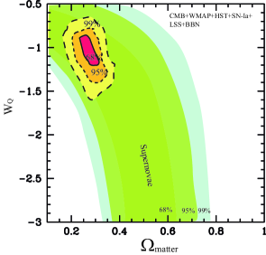
Figure 4: Likelihood contours in the ($\Omega_{M}$, $w_{Q}$) plane for the joint CMB+HST+SN-Ia+2dF analysis described in the text. We take the best-fit values for the remaining parameters. The contours correspond to 0.32, 0.05 and 0.01 of the peak value of the likelihood, which are the 68%, 95% and 99% confidence levels respectively. Also plotted are the likelihood contours from type-Ia Supernovae alone.

V Conclusions

In this paper we have provided new constraints on the dark energy equation of state parameter $w_{Q}$ by combining recent cosmological datasets. We find $-1.38<w_{Q}<-0.82$ at the $95\%$ confidence level, with best-fit model $\Omega_{M}=0.27$ and $w_{Q}=-1.05$. A cosmological constant is a good fit to the data. When comparison is possible (i.e. restricting to similar priors and datasets), our analysis is compatible with other recent analyses of $w_{Q}$ (e.g. see Spergel:2003cb , rachel and references therein), however, our lower bound on $w_{Q}$ is much tighter than the one recently reported in mortsell . In particular, we found that the CMB+HST dataset can already provide an interesting lower limit on $w_{Q}$, while in mortsell no constraint was obtained. Part of the discrepancy can be explained by our updated CMB dataset with the new Archeops, Boomerang, CBI, VSA and, mostly, WMAP results. However, our CMB power spectra in Fig.1 are in disagreement with the same spectra plotted in the Fig.2 of mortsell where the dependence on $w_{Q}$ seems limited only to the large-scale ISW term.

In the range $w>-1$ our results are in very good agreement with those reported by Spergel et al. Spergel:2003cb , which is using a different analysis method based on a Monte Carlo Markov Chain and a slightly different CMB dataset.

We found that including models with $w<-1$ does not significantly affect the results obtained under the assumption of $w>-1$. In this respect, our findings are a useful complement to those presented in Spergel:2003cb .

As in Spergel:2003cb and in most of previous similar analysis the constraints obtained here have been obtained under several assumptions: the equation of state is redshift independent, the perturbations in the dark energy fluid are negligible and/or its sound speed never differs from unity in a significant way. It is important to note that our result apply only to models well described by these approximations.

We have also demonstrated that, even by applying the most current constraints on the dark energy equation of state parameter $w_{Q}$, there is much uncertainty in its value. Interestingly, there is a distinct possibility that it may lie in the theoretically under-explored region $w_{Q}<-1$. To illustrate this we have provided a specific model in which $w_{Q}<-1$ is attained, and which satisfies the assumption that $w_{Q}$ is approximately piecewise constant, as used in the data analysis. An observation of a component to the cosmic energy budget with $w_{Q}<-1$ would naturally have significant implications for fundamental physics. Further, depending on the asymptotic evolution of $w_{Q}$, the fate of the observable universe Starkman:1999pg -Huterer:2002wf may be dramatically altered, perhaps resulting in an instability of the spacetime CHT or a future singularity.

If we are to understand definitively whether dark energy is dynamical, and if so, whether it is consistent with $w_{Q}$ less than or greater than $-1$, we will need to bring the full array of cosmological techniques to bear on the problem. An important contribution to this effort will be provided by direct searches for supernovae at both intermediate and high redshifts SNAP . Other, ground-based observations LSST will allow complementary analyses, including weak gravitational lensing Huterer:2001yu and large scale structure surveys Hu:1998tk to be performed.

At present, however, while the data remain consistent with both a pure cosmological constant $\Lambda$, and with dynamic classes of models Wetterich:fm -Armendariz-Picon:2000ah ,bastero-mersini , nature may be telling us that the universe is an even stranger place than we had imagined.

- (1) P.M. Garnavich et al, Ap.J. Letters 493, L53-57 (1998); S. Perlmutter et al, Ap. J. 483, 565 (1997); S. Perlmutter et al (The Supernova Cosmology Project), Nature 391 51 (1998); A.G. Riess et al, Ap. J. 116, 1009 (1998); A. G. Riess et al. [Supernova Search Team Collaboration], Astron. J. 116, 1009 (1998) [arXiv:astro-ph/9805201]; S. Perlmutter et al. [Supernova Cosmology Project Collaboration], Astrophys. J. 517, 565 (1999) [arXiv:astro-ph/9812133].
- (2) C. Wetterich, Nucl. Phys. B 302, 668 (1988).
- (3) B. Ratra and P. J. Peebles, Phys. Rev. D 37, 3406 (1988).
- (4) R. R. Caldwell, R. Dave and P. J. Steinhardt, Phys. Rev. Lett. 80, 1582 (1998) [arXiv:astro-ph/9708069].
- (5) C. Armendariz-Picon, T. Damour and V. Mukhanov, Phys. Lett. B 458, 209 (1999) [arXiv:hep-th/9904075].
- (6) C. Armendariz-Picon, V. Mukhanov and P. J. Steinhardt, Phys. Rev. Lett. 85, 4438 (2000) [arXiv:astro-ph/0004134].
- (7) C. Armendariz-Picon, V. Mukhanov and P. J. Steinhardt, Phys. Rev. D 63, 103510 (2001) [arXiv:astro-ph/0006373].
- (8) T. Chiba, T. Okabe and M. Yamaguchi, Phys. Rev. D 62, 023511 (2000) [arXiv:astro-ph/9912463].
- (9) L. Parker and A. Raval, Phys. Rev. D60, 063512 (1999)
- (10) P.H. Frampton, astro-ph/0209037.
- (11) L. Mersini, M. Bastero-Gil and P. Kanti, Phys. Rev. D64, 043508 (2001); M. Bastero-Gil and L. Mersini, hep-th/0205271.
- (12) R. Bean and A. Melchiorri, Phys. Rev. D 65 (2002) 041302 [arXiv:astro-ph/0110472]; R. Bean, S. H. Hansen and A. Melchiorri, Phys. Rev. D 64, 103508 (2001) [arXiv:astro-ph/0104162].
- (13) I. Maor, R. Brustein and P. J. Steinhardt, Phys. Rev. Lett. 86, 6 (2001); [Erratum-ibid. 87, 049901 (2001)] [arXiv:astro-ph/0007297].
- (14) L. M. Wang, R. R. Caldwell, J. P. Ostriker and P. J. Steinhardt, Astrophys. J. 530 (2000) 17 [arXiv:astro-ph/9901388].
- (15) R. R. Caldwell, Phys. Lett. B 545, 23 (2002) [arXiv:astro-ph/9908168].
- (16) A. E. Schulz and M. J. White, Phys. Rev. D 64, 043514 (2001) [arXiv:astro-ph/0104112].
- (17) M. Ahmed, S. Dodelson, P. B. Greene and R. Sorkin, arXiv:astro-ph/0209274.
- (18) S. M. Carroll, M. Hoffman and M. Trodden, arXiv:astro-ph/0301273.
- (19) I. Maor, R. Brustein, J. McMahon and P. J. Steinhardt, Phys. Rev. D 65, 123003 (2002). [arXiv:astro-ph/0112526].
- (20) S. Hannestad and E. Mortsell, Phys. Rev. D 66 (2002) 063508 [arXiv:astro-ph/0205096].
- (21) J. Garriga and V. F. Mukhanov, Phys. Lett. B 458, 219 (1999) [arXiv:hep-th/9904176].
- (22) J. R. Bond, G. Efstathiou and M. Tegmark, arXiv:astro-ph/9702100.
- (23) A. Lewis and S. Bridle, Phys. Rev. D 66, 103511 (2002) [arXiv:astro-ph/0205436].
- (24) U. Seljak and M. Zaldarriaga, Astrophys. J. , 469, 437 (1996).
- (25) C. L. Bennett et al., arXiv:astro-ph/0302207.
- (26) L. Verde et al., Parameter Estimation Methodology,” arXiv:astro-ph/0302218.
- (27) J. E. Ruhl et al. [Boomerang Collaboration], [arXiv:astro-ph/0212229].
- (28) N. W. Halverson et al., Astrophys. J. 568, 38 (2002) [arXiv:astro-ph/0104489].
- (29) A. T. Lee et al., Astrophys. J. 561, L1 (2001) [arXiv:astro-ph/0104459].
- (30) T. J. Pearson et al., astro-ph/0205388, (2002).
- (31) K. Grainge et al., astro-ph/0212495.
- (32) A. Benoit et al. [Archeops Collaboration], A & A, submitted, 2002.
- (33) S. L. Bridle, R. Crittenden, A. Melchiorri, M. P. Hobson, R. Kneissl and A. N. Lasenby, arXiv:astro-ph/0112114.
- (34) Bond, J.R., Jaffe, A.H., & Knox, L.E. 2000, Astrophys. J. , 533, 19
- (35) M. Tegmark, A. J. S. Hamilton and Y. Xu, astro-ph/0111575 (2001)
- (36) W. Freedman et al., Astrophysical Journal, 553, 2001, 47.
- (37) D. N. Spergel et al., Determination of Cosmological Parameters,” arXiv:astro-ph/0302209.
- (38) G. Starkman, M. Trodden and T. Vachaspati, Phys. Rev. Lett. 83, 1510 (1999) [arXiv:astro-ph/9901405].
- (39) P. P. Avelino, J. P. de Carvalho and C. J. Martins, Phys. Lett. B 501, 257 (2001) [arXiv:astro-ph/0002153].
- (40) E. H. Gudmundsson and G. Bjornsson, Astrophys. J. 565, 1 (2002) [arXiv:astro-ph/0105547].
- (41) D. Huterer, G. D. Starkman and M. Trodden, Phys. Rev. D 66, 043511 (2002) [arXiv:astro-ph/0202256].
- (42) For example, the proposed SNAP mission, http://www.snap.lbl.gov/.
- (43) For example, proposed wide-field telescopes such as the Large-aperture Synoptic Survey Telescope (LSST) http://www.dmtelescope.org/
- (44) D. Huterer, Phys. Rev. D 65, 063001 (2002) [arXiv:astro-ph/0106399].
- (45) W. Hu, D. J. Eisenstein, M. Tegmark and M. J. White, Phys. Rev. D 59, 023512 (1999) [arXiv:astro-ph/9806362].