Detached double-lined eclipsing binaries as critical tests of stellar evolution

Detached, double-lined spectroscopic binaries which are also eclipsing provide the most accurate determinations of stellar mass, radius, temperature and distance-independent luminosity for each of their individual components, and hence constitute a stringent test of single-star stellar evolution theory. We compile a large sample of 60 non interacting, well-detached systems mostly with typical errors smaller than 2% for mass and radius and smaller than 5% for effective temperature, and compare them with the properties predicted by stellar evolutionary tracks from a minimization method. To assess the systematic errors introduced by a given set of tracks, we compare the results obtained using three widely-used independent sets of tracks, computed with different physical ingredients (the Geneva, Padova and Granada models). We also test the hypothesis that the components of these systems are coeval and have the same metallicity, and compare the derived ages and metallicities with the ones obtained by fitting a single isochrone to the system. Overall, there is a good agreement among the different determinations, and we provide a comprehensive discussion on the sub-sample of systems which either present problems or have estimated metallicities. Although within the errors the published tracks can fit most of the systems, a large degeneracy between age and metallicity remains. The power of the test is thus limited because the metallicities of most of the systems are unknown.

1 Introduction

The theory of stellar evolution is one of the most successful in astrophysics, and has been widely applied to phenomena ranging from stellar oscillations to the evolution of galaxies. While open and globular clusters have been the classical tests of the theory because their colour-magnitude diagrams (CMD) constrain the shape of an isochrone in detail, they are not ideal probes, since, among other things, they are contaminated by field stars, have unresolved binaries, suffer dynamical evolution, may present differential extinction, and may be distant enough to prevent very accurate determinations of their distances (see Andersen & Nordström 1999 for a recent review on the observational requirements for open clusters). Furthermore, Hipparcos measures show that there is a very fuzzy correlation, if any, between the main sequence position and metallicity (van Leeuwen 1999, Lebreton et al. 1999, and references therein), casting some doubts –at least as far as the metallicity scaling is concerned– on current stellar evolution models.

So far relatively less attention has been paid, in comparison, to binary systems. Yet these systems provide the only way to measure directly stellar masses, and, if the components do not interact strongly and suffer mass transfer, they should have independent evolution and be representative of single stars. Visual systems are hampered by the lack of radial velocity measures (but see Pourbaix 2000), and hence mass ratios are measured indirectly (e.g. Fernandes et al. 1998 for a few examples). Interferometric systems, although promising, are too few to provide a good sample (e.g. Hummel et al. 1995, 2001, Torres et al. 2002). In this context, double-lined eclipsing binaries provide the most accurate determinations of stellar radii, masses and temperatures, and hence are ideal stringent tests of the theory, as first pointed out by Strömgren (1967) (see also Andersen 1997). Testing evolutionary tracks is important not only for the understanding of the properties of the stars, but also to assess the uncertainties in, for example, the interpretation of the spectro-photometric properties of galaxies, from low to high redshifts, or the chemical evolution of our Galaxy.
Although only a handful of systems are extremely well-measured (see below), with typical errors in masses and radii of less than 2 per cent (Andersen 1991), the sample of systems is bound to increase in the near future, with dedicated observing programs (at the Danish 50cm SAT, see Clausen, Helt & Olsen 2001; Elodie at OHP, e.g. Kurpinska-Winiarska & Oblak 2000), the analysis of Hipparcos data (e.g., Fabricius et al. 2002), the systematic detections of thousands of systems as a by-product of microlensing surveys (see, e.g., Alcock et al. 1997, and Ferlet, Maillard & Raban 1997 for an overview), and with future space missions such as DIVA, SIM and GAIA. In addition, these systems have accurate absolute dimensions and provide another distance indicator, independent of any distance calibration (e.g. Paczyński 1997, Fitzpatrick et al. 2002). However, in practice, the power of the test using these systems is limited by the small volume in parameter space sampled by most of the published theoretical tracks. For instance, many tracks adopt a single helium abundance $Y$ for a given metallicity $Z$, and do not consider any possible dispersion, while others fix the overshooting parameter or the mixing length parameter to prescribed values. Even though these values provide good fits to the colour magnitude diagrams of clusters, it is likely that these parameters change with stellar mass or metal abundance. The extant (and growing) sample of binaries will yield extremely important constraints on these parameters (and their possible correlations) when tracks with a wider range of properties will be available.
The aims of this paper are three-fold. First, we want to test whether current evolutionary tracks can account for the properties of these extremely well measured systems. This is a requisite before using them for further inferences. Even though a given set of tracks may seemingly give good results, and provide good fits, it will not produce an absolute determination because of the underlying hypotheses used in the computation of the tracks. For instance the determination of the Helium abundance relies critically on the effective temperature scale, and so different tracks, using different scales, may yield different abundances or ages. To assess the possible systematic effects introduced by a given set, we take three widely-used sets of tracks which have been computed independently and with different physical ingredients. For the same data set, which includes only the best measured stars currently available, are these sets consistent with each other?

Secondly, we want to test to which extent stellar evolution is a predictive theory, in the sense that given some observables it can predict the remaining ones, if the predictions are unique. This relies on the so-called Vogt-Russell theorem (Vogt 1926) which states that stars of the same chemical composition (and hence same opacity and energy generation rate) have radii, effective temperatures and luminosities solely determined by their masses. Although this theorem has been widely criticized, mainly because counterexamples were found (albeit in rather contrived situations, see e.g. Lauterborn 1972, 1973; Kähler 1978), it remains the basis of stellar evolution theory and is implicitely assumed in all analyses of stellar evolution data. As far as we know, no tests have been carried out to assess empirically the validity of this theorem. So, given, say, a luminosity and effective temperature, can the tracks provide a unique value for the mass and the radius? Are these values consistent with the measured ones? Allende Prieto & Lambert (1999) found that one set of tracks was able to reproduce, assuming solar metallicity, radii and masses with errors smaller than 8%, and effective temperatures within 2% for mainly main sequence stars. In a different study, Young et al. (2001) found agreement with the measured radii within 3%, and temperatures within 4% but luminosities could only be reproduced to 11% with their set of tracks. Are these figures the same for other published tracks or for stars with lower gravities?

Furthermore, and this is the third and main goal of the paper, can these sets of tracks predict the ages and metallicities of these systems? Proper testing of the accuracy of stellar dating has not yet been done before in detail (see e.g. von Hippel et al., 2001 for a summary). The components of these detached systems provide an ideal sample not only to properly calibrate the stellar tracks, but also to assess the uncertainties in the stellar ages used for the study of the evolution of our Galaxy. For instance Edvardsson et al. (1993) used a set of tracks from VandenBerg (1985) with a fixed set of physical parameters, and succeeded in reaching an accuracy of about 0.1 dex in the relative dating of F dwarfs. We want to assess whether this accuracy is robust to changes in the evolutionary tracks. In this context it is curious to observe that there has been no systematic test to see whether the components of these systems are indeed coeval. Popper (1997) observed that some secondary stars between 0.7 and 1.1 $M_{\odot}$ appeared systematically older (by at least a factor of two) than their primaries. Are the ages derived for each component consistent with them being on a single isochrone? Are their metallicities the same? What are the uncertainties (including systematics) in the absolute ages?

This paper presents the sample, the method and the detailed fits, discusses the implications of the results on the coevality of the components, the ages and metallicities inferred, and their relation to the chemical evolution of the Galaxy. When relevant we also present comparisons with the results obtained by Pols et al. (1997), Ribas et al. (2000), and Young et al. (2001), hereafter referred to as P97, R00 and Y01 respectively. Section §2 briefly describes the physical properties of the tracks used in the analysis of the data, which are presented in Section §3. Section §4 deals with specific issues related to some interesting binary systems, and Sect §5 discusses the general results and provide new photometric [Fe/H] constraints. The conclusions are presented in Section §6.

2 Evolutionary tracks

Ideally tracks with a wide range of physical parameters (not only $Y$ and $Z$ but also overshooting and convection parameters) should be used to properly test the different correlations between the parameters and the inferred ages and metallicities of the systems, so that proper statistical uncertainties can be assessed. Previous analyses (e.g. P97, Allende Prieto & Lambert 1999, R00, Y01) have relied on a given set, so cross-comparisons and systematics are difficult to assess. It is unfortunate that there is presently no published set of tracks that fully fulfill this condition and we are limited to use different sets. In this study, we adopted three widely-used tracks computed by (1) the Geneva group (Schaller et al. 1992, Schaerer et al. 1993ab, Charbonnel et al. 1993, Mowlavi et al. 1998) which will be referred to collectively as the Geneva tracks, (2) the Padova group (Bressan et al. 1993, Fagotto et al. 1994abc), and (3) the Granada group (Claret & Giménez 1992, hereafter CG92) evolutionary stellar models for a smaller range in metallicity than the Geneva and Padova ones. Table 1 summarizes the main physical ingredients that characterize these different tracks. We wish to emphasize that our main concern here is to present and validate a general method whichever the models used, but not to test all the available (or the most recent) tracks: we only choose three different sets in order to understand and quantify possible systematic effects introduced by a given set. Kovaleva (2001) did a similar analysis using a subset of 43 systems and the Geneva and Padova tracks. We also describe in Table 1 the older set from Hejlesen (1980ab, H80) because these tracks were often used previously for some of the systems studied here. They have a large mixing length theory (MLT) parameter ($\alpha$= 2.0), do not include overshooting or mass loss, and use the outdated Cox & Stewart (1970ab) opacities. For all these reasons we will only mention results derived from the H80 models as an historical guideline, because there is no reason to probe their validity (see comments on H80 related problems in e.g. Andersen et al. 1984). Some important points to note are the following :

Table 1: Basic properties of the Geneva, Padova, Granada and H80 tracks

	Geneva			Padova			Granada			H80 ${}^{a}$
	$Y$	$Z$	Ref.	$Y$	$Z$	Ref.	$Y$	$Z$	Ref.	$Y$	$Z$
				0.230	0.0004	P94a				0.2996	0.0004
	0.243	0.0010	G92
	0.252	0.0040	G93b	0.240	0.0040	P94b				0.296	0.0040
										0.196	0.0040
	0.264	0.0080	G93a	0.250	0.0080	P94b
							0.267	0.0100	CG92	0.290	0.0100
Chemical	0.300	0.0200	G92	0.280	0.0200	P93	0.280	0.0200	CG92	0.380	0.0200
composition										0.280	0.0200
										0.180	0.0200
							0.321	0.0300	CG92	0.270	0.0300
	0.340	0.0400	G93c							0.360	0.0400
										0.260	0.0400
				0.352	0.0500	P94a
	0.480	0.1000	G98	0.475	0.1000	P94c
Opacities	RI92, K91, IRW92,			IRW92, H77, CS70 ${}^{c}$			RI92, A92 ($=$AF94),			CS70
	IR96, AF94 ${}^{b}$						H77, W90 ${}^{d}$
MLT $\alpha$	1.6			1.63 [1.5 for $Z$$=$0.1]			1.5			2.0
$\Lambda_{c}$	0.2			0.2			0.2			none
Mass loss	yes			yes			yes			none

${}^{a}$ Chemical composition ($Y$, $Z$) from Hejlesen (1980b).

${}^{b}$ For $Z$ = 0.001, 0.008 and 0.020, opacities are from Rogers & Iglesias 1992 (RI92). At low temperatures, from 6000 K to 2100 K, they have completed the tables of RI92 with the atomic and molecular opacities of Kurucz 1991 (K91). For $Z$ = 0.004 and 0.040, the OPAL radiative opacities (Iglesias et al. 1992, IRW92) are used. These tables are also completed at low temperatures with K91. For $Z$ = 0.1, opacities are from Iglesias & Rogers 1996 (IR96), along with the opacities from Alexander & Ferguson 1994 (AF94) at low temperatures.

${}^{c}$ Because the OPAL tables of Iglesias et al. 1992 (IRW92) do not extend below 6000 K and above $10^{8}$ K, the opacities at lower and higher temperature, respectively, are taken from the LAOL tabulations by Huebner et al. 1977 (H77) and Cox & Stewart 1970a,b (CS70). In general, the OPAL are significantly higher than the LAOL in two temperature ranges (a few $10^{5}$ K and $\sim$ $10^{6}$ K).

${}^{d}$ Opacities are taken from RI92, but for T${}_{\mathrm{eff}}$ $<$ 6000 K or T${}_{\mathrm{eff}}$ $>10^{8}$ K they have used Alexander 1992 (A92, published later as Alexander & Ferguson 1994, AF94) opacities and Los Alamos Opacity Library – LAOL – (Huebner et al. 1977 [H77], Weiss et al. 1990 [W90]) respectively.

• Masses. For the 6 metallicities available in the Geneva tracks, the mass range is from 0.8 to 120 M${}_{\odot}$ (0.8 to 60 M${}_{\odot}$ for $Z=$ 0.1), while for the 6 metallicities in the Padova tracks the mass range is 0.6 to 120 $M_{\odot}$ (restricted to the range 0.6 to 9 M${}_{\odot}$ for $Z=$ 0.1). The CG92 grids cover masses from 1.0 to 40 M${}_{\odot}$ with 3 different metallicities. The CG92 upper mass limit is large enough for the purpose of this work because the most massive component is a 32 M${}_{\odot}$ star (namely DH Cep).

• Mass loss. The Geneva tracks use the mass loss rates given by De Jager et al. (1988) and Nieuwenhuijzen & De Jager (1990) for Pop. I stars. The Padova tracks set a mass loss rate only for stars more massive than 12 M${}_{\odot}$  (from De Jager et al. 1988) with a metallicity dependence given by the prescription of Kudritzki et al. (1989). No mass loss by stellar winds is taken into account for the $Z=$ 0.1 Padova tracks. Mass loss is also included in the CG92 tracks following Nieuwenhuijzen & De Jager (1990) and Reimers (1977) for cool giant stars.

• Nuclear rates. The main difference between the Geneva and Padova tracks is the ${}^{12}C(\alpha,\gamma)^{16}O$ reaction which occurs during the helium burning phase, causing differences in the blue loop extension in the HR diagram. The Padova tracks include the nuclear reaction rates of Caughlan & Fowler (1988) which are somewhat smaller than the rates used by the Geneva group (Caughlan et al. 1985).

• Overshooting. Although the nominal overshooting parameter $\Lambda_{c}$ of the Padova tracks is 0.5, this is just due to a different definition, and, as Fagotto et al. (1994a) explain, this value is equivalent to an overshooting distance of $\Lambda_{c}$(Geneva) $=$ 0.2 pressure scale heights. Claret & Giménez (1992) have also adopted $\Lambda_{c}$ $=$ 0.2. To test the influence of overshooting on the results we also use Geneva tracks without overshooting. However these models cover only the mass range [0.8–1.25] M${}_{\odot}$ and hence limit the application of the test to the few systems in this mass range.

2.1 Ages

One important definition which is not only semantic is the age of a star. Although some prescriptions use the start of the collapse of the parent cloud, we adopt here the convention of assigning a ‘zero age’ to the main sequence. The reason for this is twofold. First, the collapse phase is still poorly understood, and accretion processes before or during the Hayashi phase could well modify the time of arrival on the main sequence. Second, it seems simpler to follow the traditional definition of a ZAMS, a ’Zero-Age’ Main Sequence precisely when the radius of the star reaches a minimum value. To avoid any possible confusion, we hence define an ‘age’ $\tau$ as the time elapsed after reaching the ZAMS, in logarithmic units :

$$\tau=\log(t-t_{\rm ZAMS})$$ (1)

where $t$ is the actual (unknown) age and $t_{\rm ZAMS}$ the age when the star reaches the ZAMS (also unknown in absolute terms), both measured in years. We stress again that the actual age is meaningless unless a well defined reference epoch is agreed on, and all the physical processes along the pre-MS evolution are fully understood and quantified.

The Padova and CG92 tracks do follow the convention of adopting $t_{\rm ZAMS}\equiv$ 0, while the Geneva tracks do not. The dependence with mass and metallicity of the ratio $t_{\rm ZAMS}/t_{\rm TAMS}$ (where TAMS is the Terminal Age Main Sequence i.e. central hydrogen exhaustion) for these tracks shows that for all practical purposes the non zero $t_{\rm ZAMS}$ constitutes a small correction of about 2% for evolved systems, but that is important for the youngest systems. All the ages derived in the present work are post-ZAMS, i.e. we explicitely substract $t_{\rm ZAMS}$ while dealing with the Geneva tracks. The H80 tracks seem to set $t_{\rm ZAMS}=0$ for all masses.

2.2 Metallicities

The set of tracks used in this paper do not have helium abundances $Y$ independent of the metallicity $Z$ (except those from H80), but rather follow the usual prescription of increasing $Y$ for larger values of $Z$, roughly like $Y=0.23+(3.0\pm 1.0)Z$ (see e.g., Timmes et al. 1995). As shown in Table 1, the Geneva, Padova and CG92 tracks adopt different enrichment prescriptions. This means that the metallicity $Z$ derived from a given set cannot strictly be compared with the $Z$ derived from another set, since the different helium abundance will effectively mimic a slightly different $Z$. This effect has to be kept in mind when comparing the derived metallicities from the fits.

Usually, a simple relation is adopted between $Z$ and [Fe/H]: [Fe/H]$=$ log($Z$/$X$)$-$log($Z_{\odot}$/$X_{\odot}$) (where we adopt solar abundance from Grevesse, 1997, priv. comm.: $Z_{\odot}$$=$0.017 and $X_{\odot}$$=$0.713). However for low metallicity stars, the abundance of heavy elements cannot be simply derived from spectroscopic measurements of [Fe/H] because Oxygen (O) and $\alpha$ elements (Ca, Ne, Mg, S, Si) are overabundant in comparison to Iron (Fe). Therefore, because we may have to consider low metallicities for some stars in our sample, throughout this paper we consider the correction proposed by Pagel (1996),

$$Z_{\rm corrected}=Z\,\times\left[0.638f_{\alpha}+0.362\right]$$ (2)

where f${}_{\alpha}$ is a correction factor for O and the $\alpha$ elements:

$$f_{\alpha}=\left\{\begin{array}[]{lcrrl}10^{0.4}&{\rm for}&&{\rm[Fe/H]}&\leq-1\\ 10^{0.4\times{\rm[Fe/H]}^{2}}&{\rm for}&-1<&{\rm[Fe/H]}&<+0\\ 1&{\rm for}&&{\rm[Fe/H]}&\geq+0\\ \end{array}\right.$$ (3)

3 Methodology

3.1 The sample

We have compiled a comprehensive list of 60 double-lined eclipsing binaries (EBs) which have the most accurate masses, radii and temperatures found in the literature. The core of the sample is the large catalogue from Andersen (1991, hereafter A91), which is supplemented with 11 systems. We also add three other systems with slightly lower accuracy criteria which can be used for a posteriori testing. A few systems have more recent and accurate measures than those listed by A91. We have used the updated parameters for 5 systems and for the EW Ori secondary component. It is worth noting that we kept all the systems from the Andersen list even EK Cep whose secondary component is in a pre-MS phase (which is not included in the stellar tracks that we used) because our method presented in §3.3 can provide interesting results from the primary alone.

Figure 1: HR diagram for the sample of 58 binary systems with components more massive than 0.6 M${}_{\odot}$. ZAMS sequences computed by different authors for $Z=$0.02 are also indicated for comparison.

One possible concern is that these systems may have undergone mass transfer episodes in the past. Although in some special cases strong constraints can be placed on the evolution of the system (e.g. Daems, Waelkens & Mayor 1997), in general this confuses the issue. However in our sample this is unlikely to be the case : (1) We have computed the Roche radii of the components and checked that they were much larger than the stellar radii (Lastennet 1998, from the formula of Eggleton 1983), and (2) most of the systems are still between the ZAMS and the TAMS, and their radii should not have evolved significantly. The hypothesis of independent evolution without phases of mass transfer seems acceptable for every system in the sample, except perhaps for DH Cep. This system is an ellipsoidal variable, and the lack of eclipses makes any determination of the inclination very uncertain. Although Hilditch et al. (1996) and Penny et al. (1997) find that the system is detached, Burkholder et al. (1997) argue that the radii of the components are, according to their solution, very close to the Roche values. The uncertainties in the inclination of the orbit makes this system much less constraining.

Figure 1 shows the distribution of the sample on the HR diagram, where it is readily apparent that the systems are mostly sampling the evolutionary phases close to the main sequence. Also indicated are the ZAMS computed by different authors at $Z=0.02$, and the different prescriptions for overshooting and mass loss result in slightly different sequences for massive stars. Note that these sequences are very different (by about 0.05 dex in $T_{\rm eff}$ and 0.5 dex in $L/L_{\odot}$ in the range of $\log T_{\rm eff}$ from 4.0 to about 4.6) from the widely used sequence tabulated by Schmidt-Kaler (1982), which is no longer appropriate (Lastennet 1998).

Hereafter, each binary is associated with a number between square brackets (e.g. $\beta$ Aur [27]) corresponding to its entry in all the tables and figures throughout this paper.

3.2 Effective temperatures and luminosities

The individual stars in the sample have typical relative errors smaller than 5% for the effective temperature and relative errors smaller than 10% for the luminosity. The interest of the luminosity is that it follows directly from the temperature and radius (Stefan’s law), and hence is independent of distance. Since analyses of these systems combine spectroscopy and photometry, the T${}_{\mathrm{eff}}$s are likely to be more reliable than those in most of studies of single field stars.

For these reasons, these 2 parameters were used directly from the compilation of Andersen (1991) by different authors (e.g. Lastennet, Lejeune & Valls-Gabaud 1996, or Pols et al. 1997). However, because T${}_{\mathrm{eff}}$s (and therefore luminosities) are far more indirect and inhomogeneous quantities among the fundamental parameters, some efforts have been done to revise their determinations from photometric methods (e.g. Jordi et al. 1997, Lastennet et al. 1999a, Ribas et al. 2000, and Lastennet, Cuisinier & Lejeune 2002).

We decided however to keep the original T${}_{\mathrm{eff}}$ values from the references given in §3.1 for simplicity because a comparison of the T${}_{\mathrm{eff}}$s used by Ribas et al. (2000) and the ones used in this paper show a very close agreement for the 41 systems in common ($\sim$66% of our sample), the great majority (60 out of 82 stars) showing a difference below 2%. The T${}_{\mathrm{eff}}$ difference is less than 4% for all the components, except for 11 stars: both components of PV Cas [32], RS Cha [14], AI Hya [20], QX Car [42] and IQ Per [33], and GZ CMa A [23]. Since our results are not reliable for the first two (bad fit for [32] and pre-MS stars for [14]) the T${}_{\mathrm{eff}}$ disagreement has no influence on our conclusions, however the results derived for the latter systems ([20], [23], [33] and [42]) have to be taken with caution because the discrepancy in T${}_{\mathrm{eff}}$ would affect the luminosity as well, giving slightly different solutions. As suggested by Lastennet et al. (1999a, hereafter L99a), homogeneous determinations are highly preferred and to pick up some T${}_{\mathrm{eff}}$s in R00 and others in A91 and L99a would probably confuse even more the issue. Therefore for the purpose of this work and before a reliable homogeneous T${}_{\mathrm{eff}}$ determination for all the systems of the sample, we decide to keep the original T${}_{\mathrm{eff}}$s (see §3.1).

3.3 Fitting isochrones to binary systems

There has been a variety of methods dealing with the problem of fitting isochrones to a given system. Besides the early attempts by Lastennet, Lejeune & Valls-Gabaud (1996), Pols et al. (1997) assumed that both components are coeval and of the same metallicity and proceeded to minimize a $\chi^{2}$ functional which takes the observed masses, radii and temperatures and infers the best fit masses, common age and metallicity. Ribas et al. (2000) compute isochrones for each component, fixing each mass and gravity to the observed values, and proceed to compute a $\chi^{2}$ which minimizes the weighted difference between observed and predicted temperatures, as well as the difference between the predicted ages of each component. Because the masses are fixed to the observed values, the $\chi^{2}$ depends only on two remaining parameters, metallicity and helium content. In a recent paper, Young et al. (2001) use yet another formulation. First, they fix the metallicity to the solar value, and run specific evolutionary tracks of stars whose masses are given by the observations. Their $\chi^{2}$ functional minimizes the (sum of the squares of) residuals of luminosities and radii. Coevality is assumed, so that the $\chi^{2}$ depends only on age.

A common property of these formulations is that it is not clear whether the observed quantities are used to their best discriminant power. Also the intrinsic correlations between these quantities are not taken into account, and yet the very method of deriving these values, by relying on both photometric light curves and spectroscopic analyses, produces correlations among them. Another problem is that, for instance, masses are fixed (except in P97) to the mean observed values, so that even the observed dispersions in mass are not taken into account. Obviously the dispersion in mass should have some effect on the final fits, but this is not considered (except in the P97 formulation). Although one could argue that using $M$, $R$ and $T_{\rm eff}$ (as P97 do) is the best way to proceed (no derived –and hence less precise– quantities, such as luminosity or gravity, are used), P97 must assume coevality and same chemical composition. Stellar evolution theory is not therefore used to predict a priori values for each component. There cannot be possible discrepancies (which may well be the case, but it cannot be tested by this method). Likewise, R00 minimize the age difference between components, and derive a global metallicity and helium abundance for the systems.

In a first formulation, we want then to test whether ages and metallicities can de derived for each component independently. As a first step, we shall use here only the temperatures and luminosities of each of the components of the system. As it will be shown later on (see section §5.1) this does not make a difference in the final results. Note that because luminosity and temperature are not derived independently, the error bars in the HR diagram are highly correlated and strictly the error ellipse is always rotated (see e.g. Casey et al. 1998, for a brief discussion). To test the hypothesis that each component $i$ ($i=A,B$) of a given system has the same age and metallicity, we derive them by minimizing a functional defined by

$$\chi^{2}(M_{i},t_{i},Z_{i}) = \left(\frac{\log L(track)-\log L_{i}}{\sigma(\log L_{i})}\right)^{2}$$ (4)

$$+\left(\frac{\log T_{\rm eff}(track)-\log T_{{\rm eff}i}}{\sigma(\log T_{{\rm eff}i})}\right)^{2}$$

where the $\sigma$ are the 68% confidence level dispersions. The 3 sets of evolutionary tracks described in §2 are used to compute the isochrones by interpolating bilinearly at equal evolutionary phases in metallicity and age, and hence derive the values of $L(track)$ and $T_{\rm eff}(track)$.

Because there are 3 parameters and only 2 data values, the problem is degenerate and one could find an infinity of solutions that fit the data. Among them we seek the minimal values using the MINUIT package from the CERNLIB library (James 1994) and then explore the $\chi^{2}$ contours on a grid centred on the minimum minimorum.

Figure 2: Upper left panel: Zoom on the classical log T${}_{\mathrm{eff}}$-log(L/L${}_{\odot}$) HR diagram around the components of $\chi^{2}$ Hya [34] (Andersen 1991). In this example, an isochrone from the Geneva tracks is fitted to each component independently, without requiring equal ages or metallicities. The best fit isochrones are shown for each component (solid line : component A, dashed : component B). The isochrones derived from the HR diagram are also reported on the mass-radius diagram (upper right panel) and they show a very good fit to the very accurate masses and radii, even though these quantities were not used for the fit. Lower panels: Confidence regions in the (metallicity, age) plane at 1$\sigma$ (solid line), 2$\sigma$ (dashed line) and 3$\sigma$ (dot-dashed line) confidence levels for the primary (left panel) and the secondary (right panel) components. The triangles and diamonds indicate the ($Z,\log t$) values used in Fig. 3.

It turns out that, in practice, the mass is extremely well constrained and agrees with the measured value (see §3.4). This implies that a nearly unique solution $(t_{i},Z_{i})$ ought to be found. In practice a whole set of solutions is found, which gives the empirical limitation to Vogt’s theorem. Let us illustrate the procedure taking as an example the $\chi^{2}$ Hya [34] system. Figure 2 shows the best fitting isochrones –using the Geneva tracks– for each component : they are not identical. The extent to which they are statistically compatible depends on the confidence intervals for the metallicity and age of each of the components. The lower panels present the $\chi^{2}$ contours corresponding to the 1, 2 and 3$\sigma$ bounds in this reduced distance, that is, the $\chi_{min}^{2}+$ 1, 4, and 9 contours respectively. The degeneracy of the solutions is well illustrated here, as lower metallicity tracks fit a given component just as well at a slightly larger age, or a higher metallicity at a younger age. Note that at 1$\sigma$, a factor of 2 in metallicity is allowed, whereas the uncertainty in the age is about 0.05 dex for component A and 0.3 for component B. The difference stems of course from the fact that A is more evolved, and hence better constrained than B.

Note also that the 1 and 2$\sigma$ contours on Fig. 2 are closed : within them the Vogt theorem is clearly violated, but since their areas are relatively small, one could argue that, in practice, the theorem is valid since a measure of the metallicity of one of the components would be enough to constrain very accurately its age. Nevertheless, how different are isochrones distant 1$\sigma$ from the best solution ? Two examples are shown in Figure 3, where it is clear that even though the best fitting values for A and B are not the same (Fig. 2), at the 1$\sigma$ level they are statistically compatible. This is also apparent from the fact that the 1$\sigma$ contours of both components overlap : the ages and the metallicities of each component appear to be statistically compatible with each other.

It remains to be seen whether the ages and metallicities of each component are the same as the ones inferred from the fitting of a single isochrone to the combined A+B system. Fitting the best isochrone to the combined system is done in a similar way, but in this case the $\chi^{2}$ functional is obviously

$$\chi^{2}(t_{\rm sys},Z_{\rm sys}) = \sum_{i=A}^{B}\left[\left(\frac{\log L(track)-\log L_{i}}{\sigma(\log L_{i})}\right)^{2}\right.$$ (5)

$$+\left.\left(\frac{\log T_{\rm eff}(track)-\log T_{{\rm eff}i}}{\sigma(\log T_{{\rm eff}i})}\right)^{2}\right]$$

In this case the masses are no longer parameters (they are left free to take any value, just like the radii) and with 4 data values and 2 free parameters, we expect to find a $\chi^{2}$ distribution with 2 degrees of freedom Using again MINUIT to find the true minimum value, we form the $\chi^{2}$ grid in the metallicity–age plane and compute the 1, 2 and 3$\sigma$ bounds. Figure 4 shows a few isochrones within the 1$\sigma$ contour, and they are all compatible, at the 1$\sigma$ level, with the solutions found for each component (Fig. 2). Also illustrated are some isochrones chosen to show the effect of varying age, for a fixed $Z$, and changing metallicity, for a given age. In the case of $\chi^{2}$ Hya, metallicity effects are clearly more important, and therefore a measure of their metallicities would constrain extremely well their common age within 0.05 dex (that is, about 11% at 1$\sigma$). Note also that the solution found by Clausen and Nordström (1978) using the Hejlesen (1980) tracks is close to the 3$\sigma$ contour (Fig. 4) and is therefore highly unlikely, as expected with models using the outdated Cox & Stewart (1970) opacities (cf. §2).

Figure 3: $\chi^{2}$ Hya [34], individual components, Geneva tracks. For each component, the best fitting isochrones (from Fig. 2) along with the isochrones corresponding to the 1$\sigma$ level are indicated (dashed line : triangle; dot-dashed line : diamond, see Fig. 2).

Figure 4: $\chi^{2}$ Hya system [34], Geneva tracks. Upper panel: Confidence regions in the (metallicity, age) plane at 1$\sigma$ (solid line), 2$\sigma$ (dashed line) and 3$\sigma$ (dot-dashed line) confidence levels for both components. For the sake of completeness, the best fit obtained by Clausen & Nordström (1978) using the H80 models is also shown (square with error bars). Lower panel: Corresponding isochrones on the HR diagram (error bars from Andersen 1991) as in Fig.2. The best fit isochrone obtained with the Geneva tracks and defined by ($\log t,Z$) $=$ (8.275, 0.014) is indicated by the solid line. The 4 points on the 1$\sigma$ contour above correspond to the 4 isochrones showed in the lower panel.

The irregularly-shaped contours are due to the different evolutionary speeds and short lived phases, and may complicate the interpretation in some cases. It is important to note, also, that since the contours are somewhat diagonal, the degeneracy between age and metallicity is lifted as soon as a measure of the metallicity is made. The contours for the system are much smaller than the contours for the individual components, as could be expected from the addition of information.

The results of the fitting of, on one side, each component of the system, and, on the other hand, of the system on a single isochrone, are given in Table LABEL:tab:results, for all the sets of tracks which we have tested here.

3.4 Masses and radii: the most stringent tests of the method

To what extent these fitted isochrones are able to predict the observed values of the masses and radii? These are truly predictions from the theory, since the fit involved only luminosities and temperatures. Are the derived metallicities consistent with the observations? Metallicities will be discussed for the few cases where constraints exist in section §5.2, and here we analyse the predictions made by the fits for the entire sample to the very accurate masses and radii available (typical errors are smaller than 2% for mass and radius, except for 3 systems where typical mass errors are between 4 and 7%).

As clearly shown on Fig. 5 and 6, the correct mass an radius are predicted for each individual star from isochrone fitting in the (log T${}_{\mathrm{eff}}$, log L/L${}_{\odot}$) HR diagram. The relative error for the derived masses of each component is given in Fig. 5, for the Geneva tracks. The other tracks yield virtually the same results. Note again that the inferred mass comes from the fitting of an isochrone to the position of that component in the (log T${}_{\mathrm{eff}}$, log L/L${}_{\odot}$) diagram, without considering any other constraint. A linear regression yields $\Delta M/M_{\rm measured}=(M_{\rm derived}-M_{\rm measured})/M_{\rm measured}=(-4.2\pm 5.7)\,10^{-3}-(6.35\pm 1478.3)\,10^{-6}$ $M_{\rm measured}$, that is, both slope and systematic trend consistent with zero. The average relative error in mass is $-$0.54%, with a dispersion of 1.7%. This is a remarkable achievement for the theoretical tracks, since over this mass range we are probing stars which are almost fully convective to fully radiative stars.

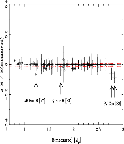
Figure 5: Relative error in mass, $\Delta M/M_{\rm measured}=(M_{\rm derived}-M_{\rm measured})/M_{\rm measured}$, inferred from the fitting of Geneva isochrones to the position of each component on the HR diagram. The dotted line is $\Delta$$M$ $=$ 0 and the dot-dashed lines are linear regressions to the data points.

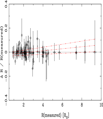
Figure 6: Relative error in radius, $\Delta R/R_{\rm measured}=(R_{\rm derived}-R_{\rm measured})/R_{\rm measured}$, inferred from the fitting of Padova isochrones to the position of each component on the HR diagram. The dotted line is $\Delta$$R$ $=$ 0 and the dot-dashed lines are linear regressions to the data points.

Only a few components (4 out of 116) present a significant discrepancy between the predicted mass and the observed one, given the error in the observed value, in Fig. 5. These are component B of AD Boo [57], both components of PV Cas [32] and IQ Per [33]. AD Boo B yields in fact a bad fit, and one cannot expect to infer a correct mass or radius from a bad fit. However, a more recent determination of the secondary component mass (M${}_{B}$$=$1.20$\pm$0.03 M${}_{\odot}$, Popper 1998) than the one we used (1.237$\pm$0.013 M${}_{\odot}$, Lacy 1997b) gives a better agreement with our theoretical predictions from the Padova (1.188$\pm$0.024 M${}_{\odot}$) or Geneva models (1.155${}^{+0.020}_{-0.022}$ M${}_{\odot}$), and even an excellent agreement with the Granada tracks: 1.205$\pm$0.025 M${}_{\odot}$.

The problem is the same for PV Cas [32], which is badly fitted by the tracks we have used. Pols et al. (1997) also obtained bad fits, even at the upper limit in $Z$ they explored ($Z=$0.03), and despite the fact that we explore a larger range (up to $Z$$\geq$0.04) we still do not manage to get a correct fit. Popper (1987) failed also to fit it with 3 other sets of models: the predicted T${}_{\mathrm{eff}}$ is too hot by $\sim$1700 K. The revised R00 T${}_{\mathrm{eff}}$s, lower by about 700 K, would give a better agreement with solar metallicity models, but as suggested by Young et al. (2001) this system may be still in a pre-MS phase, which is not taken into account in the tracks studied here.

The third, IQ Per [33] doesn’t produce a too bad fit, and, as we discussed in §3.2, adopting the R00 T${}_{\mathrm{eff}}$s would give a better agreement.

As far as the radii are concerned, Fig. 6 shows the same trend as for the masses. A linear regression yields $\Delta R/R_{\rm measured}=(-2.2\pm 1.2)\,10^{-2}+(0.8\pm 0.4)\,10^{-2}R_{\rm measured}$. The slightly positive trend is produced by a few outliers which however are not separated by the measured values by more than 1$\sigma$. Overall the mean relative error is 0.03% with a dispersion of 3.8%, again a remarkable achievement for the theoretical tracks, since we are probing stars which are almost fully convective to fully radiative stars.

Hence, the positions of these components in the HR diagram yield extremely precise and accurate predictions on their radii and masses, with dispersions of below 4% around a mean error below 0.5% both in radius and mass.

Figure 7: Using the Sun as a test case for the Padova (diamond and open star) and Geneva (circle and triangle) tracks. The adopted temperature and luminosity are 5777 $\pm$ 2.5 K and (3.844 $\pm$ 0.01) $\times$ 10${}^{33}$ erg s${}^{-1}$ (Weiss & Schlattl 1998). A bad fit (open cross) obtained with the Geneva models but with parameters close to the $Z$-$\log t$ Padova solutions is also shown for comparison.

3.5 Tests and limitations

We should however be cautious before taking these results at face, because one has to realize that these errors are only a combination of internal errors plus a fraction of external ones. Not all the systematic errors have been taken into account, nor the covariance terms in the internal, measurement errors. We will briefly mention here four important effects that one has to keep in mind when using these results: the Helium abundance, the availability of tracks with a wider range of $Z$, overshooting, and the improved accuracy of the measures.

(1) One obvious test case of a single component is the nearest star, the Sun, for which the effective temperature is known to 0.04% and the luminosity to 0.26%. Figure 7 shows the results of fitting the Sun as a (single) component using the Padova and the Geneva tracks. The very significant difference, at first sight very surprising, can mainly be ascribed to the larger He abundance used by the Geneva group in comparison to the Padova tracks as shown in Tab. 1 (Charbonnel & Lebreton 1993). The effects of the equation of state and opacities (Yildiz & Kiziloglu 1997) or diffusion (Morel et al. 1997, Weiss & Schlattl 1998) are comparatively much smaller. In the context of our work, this difference is a simple caveat not to use the published tracks blindly, and also calls for the calculation of a large grid of models with uncorrelated variations in the main physical parameters. The derived ages and metallicities are therefore track-dependent, and the values for $\sigma($Z$),\sigma(\tau)$ that we quote are necessarily lower limits because the systematic effects introduced by the tracks cannot be taken into account. The best we can do is to compare the results obtained with different tracks to assess the statistical robustness of the values derived with this procedure.

(2) For systems where the components are quite close to each other in the HR diagram, the constraints coming from the fitting of the system are weaker since there is effectively only one star as a constraint, hence increasing the degeneracy. Note that even if the contours produced by each component are similar, the best fitting values can be very different. Sometimes this difference arises from the fact that the best value is close to the boundary in metallicity allowed by the tracks. In several cases (see Table LABEL:tab:results) the fitting indicates large metallicities that can only be reached with the Padova and Geneva tracks. The best fits obtained are not necessarily good fits.

(3) The 3 sets of tracks used here have the same prescription for core overshooting (see Tab. 1). Would tracks without overshooting produce worse or better fits? For instance, P97 argue that a few systems can only be fitted with models which include overshooting. We have used Geneva tracks without overshooting for this test, and as shown in Tab. LABEL:tab:results, we find no significant differences between the Geneva models with and without overshooting. However, the power of the test is limited by the small mass range (and hence the number of systems) in common for these two sets of models, and by the fact that most of these systems yield bad fits (see §4.3). We cannot conclude, on the basis of these tracks and this small sample, whether overshooting is preferred or not. This is yet another source of systematic uncertainty that is difficult to quantify.

(4) To what extent the age–metallicity degeneracy can be partially lifted by increasing the accuracy of the measures? A good example is provided by V539 Ara [41] (§4.5.2 and Fig. 22), where the measures from Clausen (1996) are a factor of about two better than the previous ones from Andersen (1983). The degenerate areas in the ($t,Z$) plane are substantially reduced, although large metallicity solutions are allowed. See also the case of $β$ Aur [27] (§4.4.10 and Fig. 20) for a similar example. Once again, the most contraining systems are those with evolved components, even though the precision in the parameters could be worse.

4 Analysis of individual systems

We have applied the techniques developed in §3 to the entire sample of 60 systems. The results are summarized in Table LABEL:tab:results for 58 systems (from [2] to [59]) using the 3 different sets of tracks described in §2. The two remaining systems ([1a] and [1b]) are discussed in §4.2. The column marked ’T’ indicates the track used for the fit. Note also that all ages were corrected for the finite age of the ZAMS in the case of the Geneva tracks, following Eq. (1). Although the best fit values may appear discrepant, it is essential to use the minimum and maximum values tabulated (at the $n$-th confidence level, as indicated) to test for the statistical significance of the differences.

It is beyond the scope of this paper to analyse each binary system in detail, hence in the following we only discuss a few systems which either can be compared with previous studies or present problems. Except pre-MS stars (§4.1) were good fits cannot be expected with post-MS models, bad fits were obtained in the HR diagram for stars less massive than 1.2 M${}_{\odot}$, EW Ori [3] being the most massive one. They are mainly discussed in §4.3.

4.1 Binaries with (at least) a pre-MS component: EK Cep [17] and RS Cha [14]

As expected, none of the three sets of tracks are able to fit the system EK Cep [17], because the secondary is a pre–main–sequence star and the tracks used do not include these phases. Nevertheless, since our method can use information for individual stars, we can predict from the primary alone a metallicity, which turns out to be around solar.
RS Cha [14] is also identified as a pre-MS (Mamajek et al. 2000): pre-MS tracks achieve a good fit (Palla & Stahler 2001). RS Cha will not be discussed any further due to the uncertainty on its T${}_{\mathrm{eff}}$ (see §3.2).
Finally, as suggested by Nordström & Johansen (1994a, hereafter NJ94a), AR Aur B [48] may also be a pre-MS as well. Tab LABEL:tab:results predicts a metallicity slightly sub-solar ($Z$$\sim$0.014$\pm$0.003) for the system, in agreement with the NJ94a study. We derived from synthetic photometry (L99a) a lower limit on the metallicity of the primary ($Z$$>$0.017), only marginally consistent with the theoretical results. This discrepancy may come from the chemical peculiarities of both components (Zverko et al. 1997, and references therein).

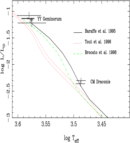
Figure 8: YY Gem [1a] and CM Dra [1b]. Data points for CM Dra come from Viti et al. (1997). The circle gives the position of YY Gem from Andersen (1991, both components at the same position), to be compared with Leung & Schneider (1978, error bars for each component) and Torres & Ribas (2002, bold error bars, both components at the same position). The isochrones of Baraffe et al. (1995) and Brocato et al. (1998) are for a solar metallicity and an age of 10 Gyr. Two analytical ZAMS ($Z$$=$0.02 and 0.03) from Tout et al. (1996) are also shown for comparison.

4.2 Binaries with VLM star components (M$<$0.7 M${}_{\odot}$): YY Gem [1a] and CM Dra [1b]

Neither YY Gem [1a] nor CM Dra [1b] provide a test for Geneva, Padova and Granada tracks, since their components are very low mass (VLM) stars, with masses below 0.6 M${}_{\odot}$. For these two systems only, we have used instead the evolutionary tracks from Baraffe et al. (1995) which are computed at $\log t=$ 10 yrs. Assuming the position of YY Gem from A91 (see Fig. 8), these tracks yield a best fit for YY Gem at $Z=$ 0.019. This is consistent with the solution found by Chabrier & Baraffe (1995), indicating also that YY Gem [1a] could be anywhere between the upper limit of 10 Gyr and the end of the pre-MS contraction phase. Since this upper limit may be too old (Torres & Ribas, 2002 estimated a younger age of $\sim$ 370 Myr), we refer the interested reader to the detailed analysis of YY Gem by Torres & Ribas (2002). We also note that using the older T${}_{\mathrm{eff}}$-L parameters from Leung and Schneider (1978) (also shown on Fig. 8) leads to virtually no constraint due to the large error bars.
Torres & Ribas (2002) adopted T${}_{\mathrm{eff}}$$=$3820$\pm$100 K (see Fig. 8) from several empirical calibrations. However, adopting the colour index values listed in their Tab. 6 for V$-$I${}_{C}$, V$-$K and (R$-$I)${}_{C}$, assuming solar abundances and the very accurate surface gravity of YY Gem from Torres & Ribas (2002), and neglecting the reddening, the BaSeL models (Lejeune et al. 1997, 1998) indicate cooler T${}_{\mathrm{eff}}$s (between 3605 and 3642 K to be compared with the coolest temperature that Torres & Ribas (2002) obtain: 3719 K from V$-$I${}_{C}$). Since the BaSeL models provide very good agreement with empirical calibrations in these colours (cf. Fig. 2 of Lejeune et al., 1998), we suspect that the T${}_{\mathrm{eff}}$s of YY Gem still need further revisions, but the temperature issue for cool stars is still controversial to give a definitive T${}_{\mathrm{eff}}$ .
In the case of CM Dra [1b], whose metallicity is compatible with the solar value (Gizis 1997) or lower (Viti et al. 1997, see also Metcalfe et al. 1996), its position in the HR diagram is very well constrained (Viti et al. 1997) for such a VLM binary, and indicates a metallicity close to solar with the models of Baraffe et al. 1995 (see Fig. 8). When using other sets of tracks (from Brocato et al. 1998, or the analytical ZAMS of Tout et al. 1996), the results are substantially different and a $Z=$ 0.02 composition is clearly inconsistent with the data (see Fig. 8). A larger sample is needed in these range of masses to confirm these tests, and the discovery of an M-dwarf eclipsing binary, GJ 2069A (Delfosse et al. 1999), with components of about 0.4 M${}_{\odot}$ (which places GJ 2069A between CM Dra and YY Gem), is a first step towards better observational constraints in the lower mass end of the main sequence (see Ségransan et al. 2000 for a recent list of accurate masses of VLM stars).

4.3 Systems with at least one component in the 0.7-1.1 M${}_{\odot}$ mass range: RT And [47], HS Aur [2], CG Cyg [46], and FL Lyr [4]

We obtain systematically worse fits for all these systems.

Figure 9: HS Aur system [2]. Left panels : Confidence regions in the (metallicity, age) plane. Right panels : HR diagrams. The top panels use the Geneva tracks, while the lower ones use the Padova ones. The best solutions obtained are indicated by circles. Keeping the same metallicity as the best solution, we also show two other points at 3$\sigma$ from the best solution, with respectively a smaller age (diamond) and a larger age (open star). Another point (triangle) is the solution with the lowest metallicity allowed at a 3$\sigma$ confidence level. The Geneva isochrones clearly do not fit the HS Aur system, no matter what age or metallicity are used. In contrast, the Padova tracks allow a successful fit at about 2.5 times the solar metallicity.

The bad fits however present two different aspects. While both components of HS Aur [2] can not be fitted (or at least only by very enriched models), the systems RT And [47], CG Cyg [46] and FL Lyr [4] have a secondary component far too cool to be matched by the same isochrone as the primary. This may reveal a different behaviour. Under the optimistic hypothesis that the location of both components of HS Aur in the HR diagram are perfectly reliable, Fig. 9 suggests that the models are unable to correctly predict its properties: either we have strong difficulties to fit both components of HS Aur (Geneva models) or we obtain very questionable metal-rich solutions (Padova models). For illustrative purposes, Fig. 9 shows that the Geneva tracks do not produce confidence areas at the 1$\sigma$ level, and most solutions are extremely far away (3$\sigma$) from the position of the system. In contrast, the Padova tracks succeed in fitting the system, but at a metallicity which is more than 2.5 times solar ($Z$$\simeq$ 0.04-0.05). This anomaly was also found by Pols et al. (1997): they obtained high $Z$ values for all systems with stars below 1 M${}_{\odot}$. The Padova tracks indicate that HS Aur is at the same time quite old and metal rich (Fig. 9, lower panels): $\sim$[Fe/H]$=$0.4-0.5. It remains to be seen whether a spectroscopic analysis confirms this predicted large metallicity.
Since the results of Pols et al. (1997) and the present study rely on the same T${}_{\mathrm{eff}}$ determination, a revision may well be needed (in particular the T${}_{\mathrm{eff}}$s of the secondary components) before definitive conclusions. Unfortunately, while L99a, R00, and Lastennet, Cuisinier & Lejeune (2002) carefully re-derive T${}_{\mathrm{eff}}$s for many EBs from photometric calibrations, none of these works study the stars in question because individual $uvby$ photometry would be necessary.
We now have to examine FL Lyr [4], CG Cyg [46] and RT And [47]. Besides a T${}_{\mathrm{eff}}$ revision, possible explanations of the disagreement may come from mass transfer and starspot activity because these 3 systems are known to be active stars. As already discussed in §3.1 none of these stars overflows its Roche lobe (see also Lastennet et al., 2002 for more details). Yet in RT And, the face-to-face position of the spots on the surface of both components may indicate the possibility of a mass transfer from the primary to the secondary component through a magnetic bridge connecting both active regions (Pribulla et al. 2000). If this is confirmed, the RT And components could not be assumed anymore to evolve like single stars, and we could not expect to reproduce their evolution with the models considered in this paper. Enhanced surface activity is also present in FL Lyr and CG Cyg. These spots lead to quite distorted light curves and consequently less well-determined photometric elements, and hence may provide an explanation of the disagreement we have found.
If the disagreements appear to remain even after further analyses, they will give additional examples to the dilemma pointed out by Popper (1997) who remarked that for systems with masses between 0.7 and 1.1 $M_{\odot}$ it was difficult to place both two components on the same isochrone. The same happens in a Mass-Radius diagram as shown by Clausen et al. (1999).
Other binaries show similar problems in this mass range, as briefly reviewed by Lastennet et al. (2002). However, the systematic differences between models and binaries of this mass range are not observed in CD Tau C, a solar mass companion of the triple system CD Tau. Ribas et al. (1999) obtained a perfect fit of the three components with a single isochrone, and the issue is still open to debate. New accurate data for low mass eclipsing binaries should help to work out the discrepancies (Clausen et al., 2001; see also Lastennet et al., 2002 and references therein).

4.4 Systems with both components in the 1.1-3. M${}_{\odot}$ mass range

4.4.1 AI Phe [5]

AI Phe is one of the most interesting systems in the sample since the coolest component is also away from the main–sequence, and observational constraints on $Z$ are available. A spectroscopic determination of metallicity from high resolution CCD spectra (Andersen et al. 1988) gives [Fe/H] $=-0.14\pm 0.1$, i.e. $Z=0.012\pm 0.003$. Using tracks from VandenBerg (1983) they derived an age of $4.1\pm 0.5\;\times\;10^{9}$ yr from isochrones with an helium abundance $Y=0.27\pm 0.02$. Our 3 sets of tracks can only fit the system at slightly lower metallicities, as shown in Fig. 10 for the case of the Geneva tracks. These results are consistent with P97 and R00. The combination of the updated parameters for the system from Milone et al. (1992) with the heavy element abundance from Andersen et al. (1988) constrain extremely well the system, with uncertainties in age smaller that 0.010 dex at 1$\sigma$ and 0.014 at 3$\sigma$. The best fit solutions are entirely compatible with both data sets. The results obtained with the Granada tracks ($Z=$ 0.011$\pm$0.001, 9.64 $<\log t<$ 9.67 yr, all 1$\sigma$) and with the Padova ones ($Z=$ $0.008^{+0.003}_{-0.000}$ and 9.59 $<\log t<$ 9.63, 1$\sigma$) are both in good agreement with the ones deduced from Geneva and the metallicity range from Andersen et al. (1988), although the range allowed in age is a bit larger.

Figure 10: AI Phe [5], Geneva tracks. The upper panels use the parameters from Andersen et al. (1988), while the lower ones take the more recent data by Milone et al. (1992). Circles (solid line isochrones) are the best solutions. In the upper panel the triangle (dashed line isochrone) is at 1$\sigma$ from the best solution. The spectroscopic metallicity ($Z=$0.012$\pm$0.003) from Andersen et al. (1988) is indicated with vertical lines.

4.4.2 UX Men [6]

This system was studied by Andersen et al. (1989) who derived a best fit isochrone of age (2.7$\pm$0.3)$\times$$10^{9}$ yr and $Y$ = 0.27$\pm$0.01 using the VandenBerg (1985) tracks fixed at $Z$ = 0.019, the observed value. There are several measures of the metallicity. Since they are consistent with each other (except that the Clausen & Grønbech value was not corrected for reddening), we adopt in Fig. 11 the more precise spectroscopic determination (Andersen et al. 1989).

Figure 11: UX Men system [6], Geneva tracks. Best fit (open circle), 1$\sigma$ points (triangles and diamonds), and a 2$\sigma$ point (open star) situated within the observed metallicity range. The vertical lines mark the observed value of $Z$ at 0.019$\pm$0.004 (Andersen et al. 1989), while the best age (open square) by Andersen et al. (1989) was derived using the VandenBerg (1985) models computed for $Z$ = 0.019. Results from Pols et al. (1997) (error bars at $Z=$0.024) and the extrapolated solution of Ribas et al. (2000) (vertical dotted line at $Z=$0.039) are also shown for comparison. The last one is unreliable because well beyond the upper $Z$-limit covered by their models ($Z$$=$0.03).

Figure 12: DM Vir system [8]. Confidence regions using the Latham et al. (1996) data and the Geneva (upper panels), Padova (middle panels) and Granada (lower panels) tracks. Best fit values (circles) are indicated in each panel, along with the corresponding isochrone (solid lines) in the HRD. Other isochrones, associated with the positions marked by triangles or diamonds on the left panels, are also shown in the HRDs. The fit obtained by Andersen, Clausen & Nordström (1984b) with the H80 tracks (open star) and by Latham et al. (1996) with the Granada tracks (square) are also indicated.

The Geneva tracks (with overshooting) give two coeval components with the same metallicity. Even though the ages are similar to the one derived by Andersen et al. (1989), the metallicity derived from the best fit is 50% larger than the spectroscopic/photometric value. This is also supported by the fitting of the combined system (Fig. 11). The Padova tracks give a very similar result, ($\log t,Z$) = (9.257, 0.034), but the Granada models and P97 yield a slightly smaller metallicity (($\log t,Z$) = (9.405, 0.027) and (9.365, 0.024) respectively). However, at the 1$\sigma$ confidence level a value as small as $Z=$0.022 (0.025) is allowed by the Geneva (Padova) models. We suspect that a slight increase in the Helium abundance may reconcile the range inferred from its position on the HR diagram with the spectroscopically determined metallicity. Alternatively, a revision of the T${}_{\mathrm{eff}}$ may be another explanation. This will be discussed further in §5.2.

4.4.3 DM Vir [8]

Accurate data from Latham et al. (1996) have superseded the values listed by A91 for this system. Figure 12 shows the best fits obtained with the Geneva (upper panels), Padova (middle panels) and Granada tracks (lower panels), and illustrates the danger of using a single set of tracks to get all the possible solutions. The limited $Z$ range in the Granada tracks lead Latham et al. (1996) to a best fit at the $Z$ limit of the Granada models, but which is by no means unique, as shown in Fig. 12. A similar good fit was also found by Pols et al. (1997) at $Z$$\sim$0.03, which is the upper limit of the models they used. This system was not selected by R00.
Although the age is very well constrained by all sets of tracks (about 0.1dex at 1$\sigma$, see Fig. 12, left panels), solutions with metallicities ranging from 0.025 to 0.06 are not statistically rejected at the 1$\sigma$ level. Since $m_{1}$(DM Vir) $-$ $m_{1}$(Hyades) $=$ 0.001 (Andersen, Clausen & Nordström 1984b), this suggests that DM Vir has a metal content similar to the one in the Hyades. Latham et al. (1996) also take [Fe/H] $=$ 0.12$\pm$0.12, although a detailed spectroscopic analysis is needed. This would imply (with $Y_{\odot}=$ 0.27) $Z=$ 0.023$\pm$0.006, yet the best fits obtained here with the 3 sets of tracks favour much larger metallicities, especially the Padova tracks. Hence, if this metallicity is confirmed, the contours of Fig. 12 show that the Padova tracks would fail to fit the system in the HR diagram, while the Geneva and Granada ones would be consistent, provided the He abundance is as high as the one used by these models (cf. Tab. 1).

4.4.4 RZ Cha [10]

The components of RZ Cha are known to be both evolved and older than 2 Gyr (Jørgensen & Gyldenkerne 1975). Andersen et al. (1975) found $\log t$ = 9.301 with a preliminary version of H80 tracks, while we obtain ($\log t,Z)=(9.32^{+0.02}_{-0.03}$, $0.015^{+0.004}_{-0.003}$) with the Geneva tracks. As illustrated in Fig. 13, the contours resulting from the fit with the Padova and Granada models are also very similar. Yet these solutions for $Z$ are systematically smaller than the value of [Fe/H] = $-$0.02 $\pm$ 0.15, which is almost solar metallicity, $Z=$ 0.020${}^{+0.008}_{-0.006}$. In fact, the Hyades metallicity adopted by Jørgensen & Gyldenkerne was an overestimation. More recent determinations (e.g. Cayrel de Strobel et al. 1997, Perryman et al. 1998) cluster around [Fe/H]${}_{\rm Hyades}=$ 0.14 $\pm$ 0.05, so that we derive for RZ Cha : [Fe/H] $=$ $-$0.08 $\pm$ 0.05 or $Z=$ 0.014 $\pm$ 0.002. This metallicity is in very good agreement with the best fits obtained by the 3 sets of tracks, the Geneva tracks being slightly better (see Fig. 13). The extremely good constraint on the age (less than 0.04 dex at 1$\sigma$) arises from its evolved position on the HR diagram. Despite the fact that both components of RZ Cha are on the same point in the HR diagram , hence a less than optimal case (Fig. 13), it is precisely because its position lies by the TAMS, that one can derive good constraints on both metallicity and age.

Figure 13: RZ Cha system [10]. The upper panel superposes the 1$\sigma$ contours from the 3 sets of tracks, along with the best fits from Geneva (open circle), Padova (square) and Granada (triangle) tracks. The metallicity range found by Jørgensen & Gyldenkerne (1975), corrected for the updated Hyades metallicity, is indicated by the vertical lines. The best fit isochrones from the three sets of tracks are shown in the lower panel.

4.4.5 PV Pup [12]

The proximity of the two non-evolved components of this system in the HR diagram does not allow to define a very accurate solution: the closer the two points on the HR diagram, the larger the contours. The Geneva tracks give a best fit at ($\log t,Z)=$ (7.53, 0.040), but metallicities as low as $Z=0.015$ and ages as large as $\log t=$ 9.1 are not excluded at the 3$\sigma$ confidence level (Fig. 14). As indicated by Vaz & Andersen (1984), the H80 models allow good fits at ($\log t,Z,Y)=$ (9., 0.02, 0.18) or at (8.60, 0.04, 0.26), yet another example of the age$-$metallicity degeneracy. Nissen’s (1981) calibration of the Strömgren $\beta$ and $\delta$m${}_{1}$ indexes gives $Z=$ 0.017 (this value is a vertical line in the iso–$\chi^{2}$ diagrams in Figs. 14 and 15). For clarity, Fig. 14 shows the results with the Geneva models and Fig. 15 with Padova models. They both indicate that better fits are obtained with larger metallicities (in agreement with Pols et al. 1997: $Z>$0.028), yet isochrones at $Z=$ 0.017 are only 2$\sigma$ away from the best fits. The revised R00 T${}_{\mathrm{eff}}$s are the same ones that we use, so our high-metallicity results are unchanged. Alternatively, the simultaneous (T${}_{\mathrm{eff}}$, [Fe/H]) solutions derived from Strömgren photometry for both components of PV Pup (Lastennet et al. 1999a) give weak constraints on the metallicity (but an upper limit of [Fe/H]$<$0.24, i.e. $Z<$0.029, at 2-$\sigma$) and a rather well-defined range of T${}_{\mathrm{eff}}$ (log T${}_{\mathrm{eff}}$ between 3.86 and 3.88). This would shift the position of PV Pup in the HR diagram towards larger values of T${}_{\mathrm{eff}}$ (and hence L) and consequently would exclude all the high-$Z$ solutions.

Figure 14: PV Pup [12], Geneva tracks. Best fit (open circle at ($\log t,Z)=$ (7.53, 0.04)), 1$\sigma$ points (triangle at $Z=$ 0.04, and diamond at $Z$ around 0.025) and the VA84 solution (square with error bars) with the H80 models are shown. The $Z$ value of VA84 (derived from the Nissen (1981) calibrations) is $Z=$ 0.017 (vertical line). Two other points (filled triangle and filled diamond) are also shown at $Z=$ 0.017, with the same ages as the (open triangle) and (open diamond) isochrones respectively.

Figure 15: PV Pup [12], Padova tracks. Isochrones for the best fit (filled circle at ($\log t,Z)=$ (5., 0.04)) and for points at 1$\sigma$ away (triangle), and for four coeval points (open circles) with the best age solution but with different metallicities ($Z=$ 0.030, 0.035, 0.045 and 0.050). The VA84 solution (square with error bars) with the H80 models is also shown, along with the $Z=0.017$ (vertical line) derived from Strömgren indexes (VA84 with Nissen (1981) calibrations). Two other points (filled triangle and filled diamond) are also shown on the $Z=$ 0.017 line.

4.4.6 TZ For [18]

TZ For is a rare occurrence of a system with a sub$-$giant and a giant, and hence potentially one of the most constraining systems. Moreover, there are spectroscopic data for this binary: Andersen et al. (1991) give [Fe/H] $=+0.1\pm$0.15. The primary of TZ For is too evolved (core helium burning phase, as suggested by Claret & Giménez, 1995a and Pols et al., 1997) to be matched by Granada models, hence only results derived for the B component are given in Tab. LABEL:tab:results. The agreement around solar metallicity is quite satisfactory for the Geneva models, but seems difficult to match with the Padova tracks: the lower limit of the Padova models at the 1$\sigma$ level is only marginally consistent with a solar metallicity. In spite of the better agreement obtained with the Geneva models, a remark has to be made. The masses of the TZ For system are known with great accuracy (better than 3% for the primary and almost 1% for the secondary) and provide stringent tests: we should derive the same masses with the theoretical tracks. Thus, if we consider TZ For B which is the strongest test and fix the mass of the Geneva tracks to its measured value, Fig. 16 clearly shows that none of the tracks succeeds in fitting this star whatever the metallicity used (cf. left panel). Alternatively, if we fix the metallicity to its observed value (Andersen et al. 1991), the mass of the tracks have to be reduced by 5$\sigma$ to reproduce the mass of TZ For B (see right panel). This shows that the Geneva models do predict a metallicity consistent with the spectroscopic value, but if the metallicity is fixed they do not predict the correct mass any more with the required precision.

Figure 16: TZ For system [18]. The hottest component of TZ For, TZ For B, is a star whose mass is known to 1% accuracy (1.949$\pm$0.022 $M_{\odot}$). Geneva tracks of several metallicities (with a mass equal to the TZ For B mass) are shown, but none of them fits this component (left panel). In order to fit TZ For B with the observed metallicity, the mass has to be reduced by 5$\sigma$ (right panel).

4.4.7 VV Pyx [19]

The best isochrone solution found with the Padova tracks gives $(\log t,Z)=$ (8.721, 0.008) while the Geneva tracks predict $\log t=$ 8.753$\pm$0.04 also at the same metallicity. The Granada tracks give solutions in good agreement with Padova and Geneva: $(\log t,Z)=$ (8.76$\pm$0.04, 0.010$\pm$0.001), see Fig. 17. It is unfortunate that there is no metallicity indications, because Andersen, Clausen & Nordström (1984a) derived a solution with a metallicity twice as large ($\log t,Z)=$ (8.6, 0.015) using the H80 models. The difference in the solutions certainly arises from the different physical ingredients of these tracks with respect to the sets we have used, as explained by Andersen et al. (1984). A measure of [Fe/H] would therefore be an ideal test here, even though spectra may be contaminated by the visual companion, a main$-$sequence A5$-$A7 star, itself perhaps a spectroscopic binary (Andersen, Clausen & Nordström 1984a). The results we derived from the HR diagram would be unchanged with the T${}_{\mathrm{eff}}$s of Ribas et al. (2000), because the revision is tiny ($\Delta$T${}_{\mathrm{eff}}$$=$22 K). An attempt to derive [Fe/H] from the synthetic BaSeL photometry (Lastennet et al. 1999a) suggests a metallicity markedly smaller than solar ([Fe/H]$<-$0.45, i.e. Z$<$0.007), but the fit of Strömgren colours and $\log g$ is bad. While this bad fit may reveal a problem of the BaSeL models, incorrect colours may be an alternative explanation, supported by the possible contamination of the visual companion.

Figure 17: VV Pyx system [19]. Comparison between the best fits obtained using the Geneva (circle), Padova (square) and Granada (triangle) tracks, superimposed on the confidence regions of the Geneva tracks. The best solutions of Andersen, Clausen & Nordström (1984a) using the H80 models (diamond) and Pols et al., 1997 (error bars) are also shown. The photometric constraint on [Fe/H] (Lastennet et al. 1999a) is shown as a solid line with arrows.

4.4.8 V1647 Sgr [22]

Andersen & Giménez (1985) used the H80 models to derive best fits between ($\log t,Z,Y)=$ (8., 0.03, 0.27) and (8.30, 0.02, 0.23). With the Geneva tracks, we get an age consistent with these results ($\log t\sim$ 8.24), but a solar metallicity ($Z=0.017$), even though a larger metallicity (say $Z=0.023$) at a slightly smaller age is not excluded by the $\chi^{2}$-contours. The Padova models agree with these values (see Fig. 18): $\log t\leq$ 8.40 and $Z=0.014^{+0.019}_{-0.002}$ as well as the Granada tracks : $\log t\in$ [7.50, 8.62] and $Z=0.016^{+0.004}_{-0.002}$. Andersen & Giménez (1985) quote a possible observed range for $Z$ between 0.02 and 0.04, which is consistent with the 3 sets of tracks used here, although smaller values are permitted. If the lower limit of $Z\geq$ 0.02 is confirmed, the Granada tracks may not be able to fit the properties of this system.

Figure 18: V1647 Sgr system [22], Padova tracks. Upper panel: $\chi^{2}$ contours in the (metallicity, age) plane. Note the shift in metallicity between the best solution from Padova tracks (open circle at ($\log t,Z)=$ (8.38, 0.014)) and the best fit by Andersen & Giménez (1985) (square with error bars) using the H80 models. The two other points (triangle and diamond) define the two corresponding isochrones (dashed line and dot–dashed line respectively) in the lower panel. Lower panel: Best fitting Padova isochrone (solid line), along with two isochrones at 1$\sigma$.

Note however that the rotation velocities of the components are not negligible ($v\sin i)_{A}=80\pm 5$ km s${}^{-1}$ and $(v\sin i)_{B}=70\pm 5$ km s${}^{-1}$ (Andersen & Giménez 1985) and that isochrones incorporating rotational effects would give slightly younger ages and larger metallicities. It has also been pointed out that the parameters of this system may have been perturbed by the presence of its bright visual companion, and this has not been taken into account in the error budget (Ribas et al. 1998).

Table 2: Comparison of age ($\log t$, in yrs.), metallicity ($Z$), and helium abundance ($Y$) determinations obtained for YZ Cas [25].

Tracks	$\log t$		$Z$		$Y$${}^{({\dagger})}$		Reference
Mengel et al. (1979)	8.544$\pm$	0.004	0.027$\pm$	0.003	0.30$\pm$	0.02	(1)
Hejlesen (1980a,b)	8.613${}^{+0.040}_{-0.044}$		0.03$\pm$	0.01	0.30$\pm$	0.04	(1)
Mengel et al. (1979)	8.8$\pm$	0.1	0.010$\pm$	0.005	0.30$\pm$	0.05	(2)
Hejlesen (1980a,b)	8.5$\pm$	0.1	0.015$\pm$	0.005	0.335$\pm$	0.050	(2)
de Loore et al. (1977)	8.65$\pm$	0.10	0.015$\pm$	0.005	0.335$\pm$	0.050	(2)
Celikel & Eryurt-Ezer (1989)	8.77$\pm$0.02		0.021${}^{(\star)}$		0.240${}^{(\star)}$		(3)
Pols et al. (1998) STD	8.66$\pm$0.02		0.014${}^{+0.004}_{-0.003}$		0.268${}^{+0.008}_{-0.006}$		(4)
Pols et al. (1998) OVS	8.70$\pm$0.02		0.016${}^{+0.006}_{-0.004}$		0.272${}^{+0.012}_{-0.008}$		(4)
CG${}^{(a)}$	8.654$\pm$0.014		0.016$\pm$0.004		0.270$\pm$0.026		(5)
CG92${}^{(b)}$	8.73${}^{+0.07}_{-0.19}$		0.017${}^{+0.013}_{-0.004}$		0.276${}^{+0.045}_{-0.006}$		(6)
Geneva	8.65${}^{+0.10}_{-0.17}$		0.018${}^{+0.009}_{-0.004}$		0.293${}^{+0.020}_{-0.011}$		(6)
Padova	8.62${}^{+0.09}_{-0.19}$		0.020${}^{+0.016}_{-0.007}$		0.280${}^{+0.035}_{-0.017}$		(6)
Strömgren photometry (B comp.)			0.018-0.020				(5)

${}^{(a)}$ Claret (1995), Claret & Giménez (1995), Claret (1997), Claret & Giménez (1998); ${}^{(b)}$ Claret & Giménez (1992); ${}^{(\star)}$ Assumed composition.
(1) Lacy (1981); (2) De Landtsheer & De Grève (1984); (3) Celikel & Eryurt-Ezer (1989); (4) Pols et al. (1997); (5) Ribas et al. (2000): [Fe/H]$=$0.03, i.e. $Z$$=$0.018 (assuming $Z_{\odot}$$=$0.017, Grevesse 1997, priv. comm.) or $Z$$=$0.020 (assuming $Z_{\odot}$$=$0.0188, Schaller et al. 1992); (6) This work. ${}^{({\dagger})}$ Only the CG models allow an independent determination of $Y$ and $Z$. Otherwise, $Y$ is derived from a fixed law once $Z$ is determined.

4.4.9 YZ Cas [25]

This system has been studied a lot previously, and Fig. 19 and Table 2 summarize the results obtained so far. Except for the measures of Lacy (1981), all sets of models (whatever the stellar parameters used) agree in supporting a solar metallicity ($Z$ range between 0.015 and 0.020). As quoted in Tab. 2 a solar composition is supported by photometric determination on the B component, a F2V star (Ribas et al., 2000). Even though its components are not very evolved, YZ Cas is a stringent test of the models because of the relatively large difference in its masses. The metal abundance determination of R00 is therefore a strong support to the quality of the tracks in the $\sim$ 1.3-2.3 M${}_{\odot}$ range.

Figure 19: YZ Cas [25], Geneva tracks (open circle symbol for the best fit, and 1-, 2- 3-$\sigma$ contours). For comparison, the results of previous studies are indicated: Lacy (1981) using the MDSG79 tracks (filled square) and the H80 models (filled triangle); De Landtsheer & De Grève (1984) with the MDSG79 (square), the H80 (triangle), and the De Loore et al. (1977) models (cross); Celikel & Eryurt-Ezer (1989) (filled circle). More recent studies from Pols et al. (1997) (open star), and Ribas et al. (2000) (diamond) are also shown. A metallicity estimate from photometry is indicated with vertical dotted lines. See Table 2 for further details.

Apart from this very good agreement between models and data, we have to mention that there is still an open problem concerning the primary component, YZ Cas A, a metallic Am star. While a disagreement may be expected between the atmospheric metallicity ($Z$${}_{\rm atmos.}$) and its intrinsic composition ($Z$, as derived from the models) due to an enhancement of the metal abundance in its external layers, Lastennet, Valls-Gabaud & Jordi (2001) found some discrepancy between the $Z$${}_{\rm atmos.}$ determinations. While photometric methods suggest that $Z$${}_{\rm atmos}$ is solar, $Z$${}_{\rm atmos}$ derived from IUE observations by De Landtsheer & Mulder (1983) is still high ($Z$${}_{\rm atmos.}$$=$0.036$\pm$0.005) despite the attempt of Lastennet, Valls-Gabaud & Jordi (2001) to revise some of the assumptions made by the IUE-based spectral study. More detailed analyses are needed to understand this disagreement.

4.4.10 $β$ Aur [27]

In this system we can compare the effects of increased precision in the measures of its parameters. Fig. 20 uses the $\log T_{\rm eff}$ and $\log L$ parameters listed by Andersen (1991) (upper panels) and the more recent ones from Nordström & Johansen (1994b, hereafter NJ94b) in the lower panels. The former values give $Z=$ 0.025 and $\log t$= 8.614 using the Geneva tracks, similar to the best fit values found for each component separately. These results are inconsistent with the constraints in metallicity given by Toy (1969) : $-$0.03 $\leq$ [Fe/H] $\leq$ 0, and the disagreement is even worse with the Padova tracks, since they give best fit models at $Z=$ 0.035 and $\log t=$ 8.537, although at the 1$\sigma$ level they may be compatible.

Figure 20: $\beta$ Aur [27], contours with Padova models. Upper panels : assuming the A91 values in the HR diagram, best fits with Padova (circle), Geneva (triangle) and Granada (open star) tracks. Note that the Granada value is at the upper limit available in this set ($Z=$ 0.03). Lower panels : Using the updated parameters from NJ94b, the best fit, high metallicity, Padova isochrone (open circle) is consistent with the best fit isochrones from Geneva (triangle) and Granada models (open star), even though their metallicities differ by a factor of 3. Also shown is a Padova isochrone (dashed line) of solar metallicity (open square). The diamond represents the NJ94b solution (using the Granada tracks). The observed constraints on metallicity (Toy 1969) between [Fe/H] =$-$0.03 and [Fe/H] $=$ 0 are indicated with vertical lines.

The NJ94b analysis yields two components which are well separated in the HR diagram and the constraints in the ($Z$, $\log t$) diagram are much better, as the lower panels of Fig. 20 show. The uncertainty regions are greatly reduced and the solutions are shifted towards smaller metallicities. Nordström & Johansen (1994b) obtained $Z=$ 0.015 and an associated age of $\log t=$ 8.75. The solutions obtained here with the Geneva ($Z=$ $0.014^{+0.006}_{-0.004}$), Padova ($Z=$ $0.066^{+0.010}_{-0.059}$, see Fig. 20, lower panels) and Granada ($Z=$ $0.017^{+0.002}_{-0.005}$) tracks are all in good agreement and consistent with the metallicity constraint of Toy (1969). Note however that there is an island of solutions at high metallicity and smaller age that remains with the Padova tracks, giving rise to isochrones that are statistically indistinguishable from the lower $Z$ ones (see the left bottom panel in Fig. 20). This island is in principle excluded because the implied metallicity is much larger than the observed one, although a modern spectroscopic determination would be useful to confirm Toy’s (1969) values.

4.4.11 V1031 Ori [28]

All the models converge towards the same solution for this system. Andersen, Clausen & Nordström (1990) used two sets of tracks and derived ($\log t,Z,Y$) = (8.74, 0.024, 0.27) with VandenBerg’s (1985) models and ($\log t,Z,Y$) = (8.85, 0.02, 0.28) with the older generation of Geneva models (Maeder & Meynet 1988, 1989). The updated Geneva tracks give a best fit at ($\log t,Z$) = (8.771, 0.021), while the Padova tracks indicate ($\log t,Z$) = (8.747, 0.020), in agreement with Pols et al. (1997), ($\log t,Z$) = (8.79, 0.023), and Ribas et al. (2000), ($\log t,Z$) = (8.846, 0.016). Granada models favour coeval solutions with a larger metallicity ($Z\approx$ 0.027), although at the 1$\sigma$ confidence level there is no disagreement with the other sets of tracks, and with the photometric constraint derived from the BaSeL models on V1031 Ori B ($Z$$<$0.029, Lastennet et al. 1999a). Nevertheless, another photometric determination (Ribas et al., 2000) suggests a sub-solar metallicity ($Z$$\sim$0.010) which would imply a systematic problem in all the above-mentioned theoretical models for main-sequence stars around 2.3–2.5 M${}_{\odot}$. The CG models used by Ribas et al. (2000) would be marginally consistent while the others are clearly ruled out. Once again, a detailed spectroscopic analysis would be needed before further inferences.

Figure 21: GG Lup [36], Geneva tracks contours. Best fits with Geneva (circle), Padova (square) and Granada (triangle) tracks are shown, as well as the best fit by Andersen et al. (1993) (diamond, ACG93) with the Granada tracks. The data points in the HR diagram are from Andersen et al. (1993).

4.5 Systems with at least one star more massive than 3 M${}_{\odot}$

4.5.1 GG Lup [36]

For this system we use the Andersen et al. (1993) data which update the A91 review. Even though the positions of the components in the HR diagram have not changed, the accuracy has increased two- or three-fold. This improvement results in smaller uncertainty regions, but still highly elongated along the $Z$ direction (Fig. 21). Andersen et al. (1993) derived a best fit isochrone with ($Z,\log t)=$ (0.015, 7.30) with the Granada models, claiming that this metallicity is in agreement with unpublished preliminary determinations by Clausen. Our results are consistent with these values at the 1$\sigma$ level, but a much wider range in $Z$ is allowed by the evolutionary tracks. Basically all isochrones with ages younger than 5$\times 10^{7}$ yr and a metallicity between $Z$$=$0.014 and $Z$$=$0.037 can fit reasonably well this system in the HR diagram. These results are unchanged if we consider the recent T${}_{\mathrm{eff}}$ revision from R00. On the other hand, Lastennet et al. (1999a) provide a slightly hotter T${}_{\mathrm{eff}}$ (by $\sim$0.9%) and a smaller uncertainty (by a factor of 3) on the coolest component which would imply smaller contours in Fig. 21, excluding all the solutions with Z$\geq$0.025.

4.5.2 V539 Ara [41]

This system was studied by Andersen (1983), and more recently by Clausen (1996), allowing to study the influence of more accurate data on the best fit isochrones. Figure 22 uses the Andersen (1983) data in the top panels and the Clausen (1996) values in the lower panels. Both Geneva and Padova tracks give a smaller $Z$ and a larger age than previous determinations, although they all lie on the 1$\sigma$ contours. The updated values decrease somewhat the uncertainty area in the metallicity–age plane, but a large range of $Z$ is still allowed (see Fig. 22), despite the two-fold increase in the accuracy of the data. Unfortunately, as indicated by Clausen (1996), attempts to measure the metallicity are hampered by the relatively large rotational velocities of its components, respectively 75 km s${}^{-1}$ (component A) and 48 km s${}^{-1}$ (component B).

Figure 22: V539 Ara system [41]. Top panels: metallicity–age contours and HR diagram with the Andersen (1983) data. The best fitting isochrone with the current Geneva tracks (open circle, at ($\log t,Z)=$ (7.7, 0.01)) gives a smaller $Z$ and larger age than previous determinations (square: Clausen 1979 [with the Hejlesen et al. 1972 tracks]; open triangle : De Grève 1989 with overshooting; filled triangle : De Grève 1989 without overshooting [the latter two with the Prantzos et al. 1986 tracks]). Lower panels: The same as above, but with the more recent values from Clausen (1996) and tracks from Geneva (G.) and Padova (P.). The diamond represents the best fit value obtained by Clausen (1996) using the Granada tracks. The open circles (G. at ($\log t,Z)=$ (7.58, 0.017) and P. at ($\log t,Z)=$ (7.62, 0.015)) give the best fits from Geneva (full line) and Padova (dashed), while typical Padova 1$\sigma$ isochrones (filled circles) are also shown for comparison (dot-dashed lines).

The best fit values obtained by Clausen (1996) using the Granada tracks are ($\log t,Z,Y$) = (7.65, 0.02, 0.28), identical to our results (see Table LABEL:tab:results), but there are many other possible solutions given approximately by the confidence regions ($\log t,Z$) = ($7.65^{+0.08}_{-0.21}$ yr, $0.020^{+0.010}_{-0.008}$). This point emphasizes the power of the method used in the present work: the confidence regions are essential to properly assess and understand the results of the tests.

4.6 Very massive stars: M $>$ 10 M${}_{\odot}$

As quoted in 1987 by Hilditch & Bell, there were not many accurate systems in this mass range, and this is unfortunately still true: only 7 systems of our working sample fall in this category, namely (by increasing order of mass) CW Cep [43], AH Cep [51], V478 Cyg [44], Y Cyg [50], EM Car [45], V3903 Sgr [52] and DH Cep [53]. The main reason is that the MS lifetime of such massive stars is short, and so these binaries are often observed during their interacting phase of evolution, excluding them from our sample of well-detached systems.

All these systems have good fits, and the more massive ones ($\geq$ 15 M${}_{\odot}$, which then excludes CW Cep and AH Cep) seem to yield low metallicities. As mentioned earlier on (§3.1), DH Cep may have overflown its Roche lobe, and we exclude it from further discussion (even though it follows this trend of lower $Z$ as well). Previous studies with different fitting methods also show the same trend: extrapolated solutions at $Z=$ 0.009 for V478 Cyg, Y Cyg and EM Car, with a possibly even lower $Z$ for Y Cyg according to its bad fit (Pols et al., 1997), $Z=$0.005 for EM Car and $Z=$0.010 for V3903 Sgr (Ribas et al., 2000).

Can new and carefully derived temperatures change this low metallicity trend? The revised temperatures of Ribas et al. (2000) leave unchanged the T${}_{\mathrm{eff}}$ of V478 Cyg, EM Car, Y Cyg and V3903 Sgr and decrease by only 0.003 dex both components of CW Cep, therefore same results are expected with these new determinations. Obviously, results that can be derived for O-B binaries in the HR diagram have to be taken cautiously due to the more uncertain T${}_{\mathrm{eff}}$-scale for massive stars, and so definitive conclusions are premature. Moreover, because metal abundance is difficult to determine in hot stars, it becomes difficult to discriminate between models. For this reason, EM Car deserves more discussion because it is the only system with metallicity indications. Our theoretical predictions favour low metallicities: $Z$$=$0.003 (Geneva models) and $Z$$=$0.004 (Padova models), in agreement with Pols et al. 1997 ($Z$$=$0.009, extrapolated solution), and Ribas et al. 2000 ($Z$$=$0.005$\pm$0.002).

The metallicity constraint on EM Car is [Fe/H]$<$0.10, as inferred from the photometry of its secondary component, and favours low metallicity solutions ([Fe/H]$=-$0.90, i.e. $Z$$\sim$0.004). This result is obtained from photometric calibration (BaSeL library) matching the very accurate surface gravity (log g$=$3.928) and the observed dereddened colours (b$-$y)${}_{0}$, m${}_{0}$, and c${}_{0}$ (Lastennet et al. 1999a), and supports the inferred low-$Z$ trend mentioned above.

Alternative explanations for low metallicities in massive binaries may come from the fact that the models may be too dim, so low metallicties models can fit the data without a proper physical reason (Young et al. 2001). However, while Young et al. (2001) and our results do use the information on the luminosity, this do not explain the low-$Z$ results of Pols et al. and Ribas et al.. Therefore the heavy element abundance may be actually small for the systems of the sample with masses larger than $\sim$ 15 M${}_{\odot}$. More accurate data for massive stars are needed to solve this issue.

5 General discussion

We discuss here the implications of the careful determinations of age and metallicity that we have obtained for most of the systems of our sample.

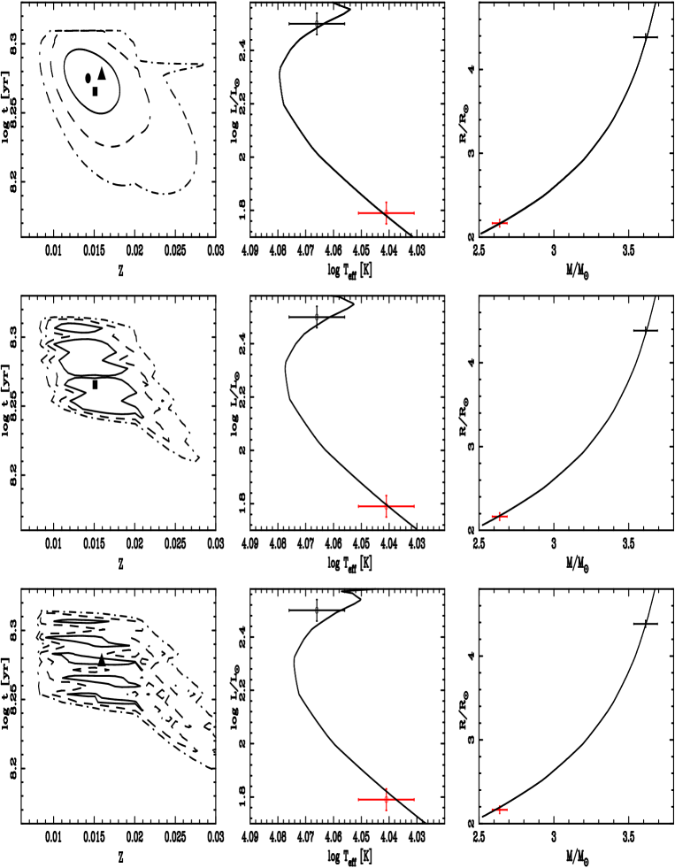
Figure 23: $\chi^{2}$ Hya system [34], Geneva tracks. We use 3 different $\chi^{2}$-estimators to fit both components : (1) a fit matching T${}_{\mathrm{eff}}$ and $L$ (our standard formulation) (upper panels), (2) a simultaneous fit of T${}_{\mathrm{eff}}$, $L$, $M$ and $R$ (middle panels), and (3) a fit involving only $M$ and $R$ (lower panels). For each $\chi^{2}$ estimator the confidence regions in the metallicity-age plane are given (left panels), along with the resulting HR diagrams (middle panels) and Mass-Radius diagrams (right panels). For comparison, the minima obtained from each method (filled circle, square and triangle for methods (1), (2) and (3), respectively) are plotted on the upper left panel.

5.1 Possible systematic trends in age and metallicity

Before attempting to draw general conclusions from these results, it is worth asking whether the inclusion of further information would improve the determinations of age and metallicity. After all, as we showed in Section § 3.3, when fitting a single isochrone to the system, the degeneracy area in the age-metallicity plane was in general reduced, due to the extra information added (two luminosities and two effective temperatures). Would the inclusion of mass and/or radius, into the $\chi^{2}$ functional reduce the uncertainties in the final ages and metallicities? We compare here three different formulations for the $\chi^{2}$ functional : (1) our standard expression, based only on T${}_{\mathrm{eff}}$ and $L$; (2) a functional minimizing the residuals using all the information available, namely the four quantities T${}_{\mathrm{eff}}$, $L$, $M$ and $R$; and (3) a functional using only the most direct quantities $M$ and $R$. This last formulation allows us to check the predictive power of the theory on the other two parameters, T${}_{\mathrm{eff}}$ and $L$. As in §3.3, we will take the system $\chi^{2}$ Hya [34] as an example.

Each formulation is illustrated on Fig. 23 with a $Z$–$\tau$ diagram, a classical HR diagram and a $M-R$ diagram. It is immediately clear that in the ($Z$, $\tau$) plane the confidence areas are roughly similar in shape and extension, although method (2) provides slightly tighter constraints, as expected, at the 3$\sigma$ level. However in this case there are several “islands” at the 1$\sigma$ level, giving rise to multiple, unconnected solutions, which are difficult to understand given Vogt’s theorem. This multimodality also indicates that 1$\sigma$ solutions may be vastly underestimated if a local minimum (and not the absolute one) is found instead. These islands are even narrower when using $M$ and $R$ only (method 3). While method (3) makes a good fit to $R$ and $M$, it fails to provide an excellent isochrone in the HR diagram. Likewise method (2), which has no predictive power in this sense, yields somewhat worse fits in the HR diagram than method (1) which is therefore our preferred one for providing the best possible fit in the HR diagram and for predicting properly masses and radii.

At first sight, these results might be surprising: the extra information added (method 2) does not yield a vast improvement on the solution, nor do the more precise masses and radii (method 3). The addition of more information (method 2) imposes much tighter constraints on the models, and simply reveals their deficiencies in a better way. There are two possible additional reasons for this. First, all these quantities are correlated, and hence bring less information than naively expected. When we added the two components in §3.3 fitting a single isochrone, the correlations between the parameters of one component and the parameters of the other remain, but are in general much smaller than those within a single component, and therefore yield better constraints. Another possible reason is that these systems remain close to the ZAMS, where there are well-defined mass-radius and mass-luminosity relations, implying even stronger correlations, and thus even less information. Systems with components in widely-separated stages of evolution would probably make much larger differences. With the current sample of binaries, however, these different formulations yield somewhat similar results, with method (1) being preferred for yielding the best fits to $L$ and T${}_{\mathrm{eff}}$, and predicting correctly $M$ and $R$.
An important motivation for this choice is that for single stars and less constrained systems such as visual binaries, one does not have $M$ and $R$, whereas $L$ and T${}_{\mathrm{eff}}$ can be determined in many cases.

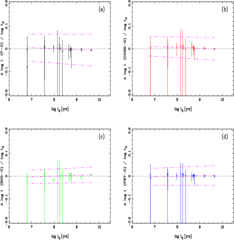
Figure 24: Relative errors in age ($\log t$) derived with Padova models (a), Granada tracks (b), R00 (c) and P97 (d), as a function of the age predicted by the Geneva tracks. The dotted line is $\Delta$$\log t$ $=$ 0 and the dot-dashed lines are linear regressions to the data points.

Another question that arises is whether the solutions found here are compatible with previous analyses, which used not only different sets of tracks, but also different $\chi^{2}$ formulations. By and large, the ($Z$,$\tau$) solutions are very similar and statistically consistent with each other. But are there any systematic trends between the different analyses? We compare here in detail our results with those obtained by Pols et al. (1997) and by Ribas et al. (2000). We do not take into account the results from Young et al. 2001 because they fixed all the metallicities to the solar value. The sub-sample in common includes only 14 systems mainly because we are restricted to $Z$$<$0.03, the upper limit considered in P97 and R00. We plot the relative differences (in the sense results with Padova, Granada, R00 or P97 minus results derived from the Geneva tracks) in age on Fig. 24. Not only the agreement between the 5 different estimations are very good, but there are no systematic effects: the average relative error in age is $-$0.49%, 0.32%, 0.29% and 0.35%, with a dispersion of 2.2%, 1.0%, 1.3% and 0.5% for panels (a), (b), (c) and (d), respectively. This is a very good result for the theoretical models considering the large individual error bars.

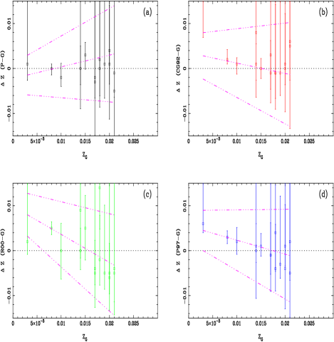
Figure 25: Error in metallicity derived with Padova models (a), Granada tracks (b), R00 (c) and P97 (d), as a function of the metallicity predicted by the Geneva tracks. The dotted line is $\Delta$$Z$ $=$ 0 and the dot-dashed lines are linear regressions to the data points.

The error in metallicity (Fig. 25) is much larger, but results are consistent within 20% for most cases, even though uncertainties remain large. The metallicity provided by the Geneva tracks is compatible with the one given by the Padova tracks (Fig. 25a). There is a slight systematic trend of the Geneva (and hence Padova) tracks with the other ones (Granada, P97 and R00) in the sense that the low metallicity systems are given a smaller metallicity by the Geneva (and Padova tracks). However this trend is produced by two stars only ($\zeta$ Phe [35] and EM Car [45]) and seems hardly significant because the P97 and R00 solutions are extrapolated for such low Z-values.

5.2 Metallicity constraints

Given that all these independent methods seem to predict consistent ages, how do the metallicity values compare to the observed ones? Obviously the most discriminant systems are those, as pointed out by Andersen (1991) and earlier references therein, which have relative errors smaller than 2% in mass, less than 1% in radius, less than 2% for temperature and less than 25% for [Fe/H]. Nearly all the binaries presented in this paper verify the two first criteria, but only 32 individual stars reach the target accuracy on T${}_{\mathrm{eff}}$. In addition, we want both components in a system to be within these limit of a 2% error in T${}_{\mathrm{eff}}$, so we have to exclude 4 systems ([18], [35], [46], [59]). The revision proposed by Ribas et al. (2000) affects some of these stars, so for extra precaution we also exclude the systems revised by more than 2% ([7], [20], [24] and [33]). Among this reduced subsample of 10 systems, we have to further exclude systems showing a bad fit in the HR diagram (see §4.3) or those for which models are unable to predict correctly the mass and/or radius (§3.4). The 7 systems selected ([3], [6], [8], [9], [11], [50], [56]) provide the best possible tests for the comparison of [Fe/H].

Many attempts have been done in the past to measure [Fe/H] in double-lined eclipsing binaries. A summary is presented in Table 3. It is somewhat distressing to note that from all the systems listed in Table 3 only UX Men [6] and DM Vir [8] belong to the sample selected above with strict accuracy criteria.

Table 3: Summary of the observational metallicities from spectroscopic analysis (sp.) or photometric calibrations in the Strömgren (S) or Geneva (G) systems. As in Table LABEL:tab:results, T (col. 7) refers to the tracks used to derive the values $Z_{tracks}$ and [Fe/H]${}_{tracks}$ given in the 2 last columns. The high metallicity results ($Z_{tracks}$) for V1143 Cyg [7] are probably unreliable: applying the revised T${}_{\mathrm{eff}}$ from R00 would give a smaller value ($Z$ in the range 0.02-0.03).

System	[Fe/H] ${}^{a}$	$Z$ ${}^{a}$	Method	Ref.	$Z_{derived}$ ${}^{b}$	T	$Z_{tracks}$ ${}^{c}$	[Fe/H]${}_{tracks}$ ${}^{b,c}$
$\beta$ Aur [27]	+0.00 ${}^{d}$		sp.	T69	0.017	1	$0.014^{+0.006}_{-0.004}$	$-0.08^{+0.16}_{-0.15}$
	$-$0.03 ${}^{d}$		sp.	T69	0.016	3	$0.066^{+0.020}_{-0.051}$	$+0.62^{+0.13}_{-1.00}$
						4	$0.017^{+0.002}_{-0.005}$	$+0.00^{+0.05}_{-0.15}$
RZ Cha [10]	$-$0.02$\pm$0.15	$0.020^{+0.008}_{-0.006}$	S	A75	$0.016^{+0.007}_{-0.004}$	1	$0.015^{+0.004}_{-0.003}$	$-0.05^{+0.10}_{-0.10}$
	$-$0.08$\pm$0.05		S	this work${}^{{\dagger}}$	0.014$\pm$0.002	3	$0.018^{+0.008}_{-0.003}$	$+0.03^{+0.16}_{-0.08}$
						4	$0.017^{+0.002}_{-0.004}$	$+0.00^{+0.05}_{-0.12}$
V1143 Cyg [7]	$+$0.08		S	A87	0.020	1	$0.040^{+0.002}_{-0.004}$	$+0.38^{+0.03}_{-0.05}$
						3	$0.050^{+0.004}_{-0.007}$	$+0.49^{+0.04}_{-0.08}$
						4	$0.030^{+0.000}_{-0.010}$	$+0.25^{+0.00}_{-0.18}$
TZ For [18]	+0.1$\pm$0.2 ${}^{e1}$		sp.	A91b	$0.021^{+0.012}_{-0.007}$	1	$0.015^{+0.004}_{-0.001}$	$-0.05^{+0.10}_{-0.3}$
	+0.14$\pm$0.15 ${}^{e2}$		sp.	A91b	$0.023^{+0.009}_{-0.006}$	3	$0.038^{+0.004}_{-0.017}$	$+0.37^{+0.04}_{-0.27}$
	+0.1$\pm$0.15 ${}^{e3}$	$0.021^{+0.009}_{-0.006}$ ${}^{f}$		A91b	$0.021^{+0.008}_{-0.006}$	4	$0.016^{+0.014}_{-0.002}$	$-0.03^{+0.28}_{-0.06}$
UX Men [6]	$-$0.15		S	CG76	0.012	1	0.031$\pm$0.009	$+0.27^{+0.12}_{-0.15}$
	+0.04$\pm$0.10	0.019$\pm$0.004 ${}^{g}$	sp.	A89	$0.018^{+0.005}_{-0.004}$	2	0.032$\pm$0.008	$+0.29^{+0.10}_{-0.13}$
	$-$0.05$\pm$0.15		S	A89	$0.015^{+0.006}_{-0.004}$	3	$0.034^{+0.010}_{-0.009}$	$+0.31^{+0.12}_{-0.13}$
	$-$0.04		G	KN90	0.015	4	$0.027^{+0.003}_{-0.007}$	$+0.21^{+0.05}_{-0.04}$
	0.1	0.024		T97
AI Phe [5]	+0.17$\pm$0.20		S	VH85	$0.025^{+0.014}_{-0.009}$	1	$0.010^{+0.001}_{-0.002}$	$-0.23^{+0.04}_{-0.10}$
	$-$0.14$\pm$0.1	0.012$\pm$0.003	sp.	A88	$0.012^{+0.003}_{-0.002}$	2	$0.009^{+0.004}_{-0.001}$	$-0.28^{+0.16}_{-0.05}$
	$-$0.1	0.012		T97	0.014	3	$0.008^{+0.003}_{-0.000}$	$-0.33^{+0.14}_{-0.00}$
						4	0.011$\pm$0.001	$-$0.19$\pm$0.04
PV Pup [12]	$-$0.06	0.017	S	VA84	0.015	1	$\geq$ 0.024	$\geq$ 0.16
						3	$0.040^{+0.032}_{-0.012}$	$+0.39^{+0.28}_{-0.16}$
						4	$\geq$ 0.021	$\geq$ 0.10
V1647 Sgr [22]		0.02-0.04	?	AG85	0.07-0.39	1	$0.017^{+0.006}_{-0.003}$	$+0.00^{+0.13}_{-0.09}$
						3	$0.014^{+0.019}_{-0.002}$	$-0.09^{+0.38}_{-0.06}$
						4	$0.016^{+0.004}_{-0.002}$	$-0.03^{+0.10}_{-0.06}$
DM Vir [8]	0.12$\pm$0.12	0.023$\pm$0.006	S	A84b	$0.022^{+0.007}_{-0.005}$	1	$0.034^{+0.021}_{-0.011}$	$+0.31^{+0.22}_{-0.17}$
	0.13$\pm$0.05		S	this work${}^{{\dagger}}$	$0.023^{+0.002}_{-0.003}$	3	$0.041^{+0.022}_{-0.013}$	$+0.40^{+0.16}_{-0.19}$
						4	$0.030^{+0.000}_{-0.011}$	$+0.25^{+0.00}_{-0.20}$

${}^{a}$ Values of $Z$ as given in the papers of column 5 (Ref.). ${}^{b}$ Adopting $Z_{\odot}=$ 0.017 and using Eq. 2. ${}^{c}$ 1 $\sigma$ confidence interval, fitting both components except for TZ For [18]: fitting only TZ For B with the CG92 tracks (T$=$4). ${}^{d}$ [Fe/H] = 0.00 for the binary and [Fe/H] = $-$ 0.03 for the secondary component. ${}^{e1}$ Mc Donald observations (A91b). ${}^{e2}$ ESO observations (A91b). ${}^{e3}$ Adopted mean by A91b. ${}^{f}$ Assuming $Z_{\odot}=$ 0.0169 (VandenBerg 1985). ${}^{g}$ Assuming $Z_{\odot}=$ 0.0189 (Maeder & Meynet 1988, 1989). ${}^{{\dagger}}$ Updade inferred from [Fe/H] $=$ [Fe/H]${}_{\rm Hyades}$ $-$ [Fe/H]${}_{\Delta m_{1}}$, by adopting [Fe/H]${}_{\rm Hyades}$$=$0.14$\pm$0.05 (Perryman et al., 1998).