Reprocessing the Hipparcos Intermediate Astrometric Data of spectroscopic binaries: II. Systems with a giant component

By reanalyzing the Hipparcos Intermediate Astrometric Data of a large sample of spectroscopic binaries containing a giant, we obtain a sample of 29 systems fulfilling a carefully derived set of constraints and hence for which we can derive an accurate orbital solution. Of these, one is a double-lined spectroscopic binary and six were not listed in the DMSA/O section of the catalogue. Using our solutions, we derive the masses of the components in these systems and statistically analyze them. We also briefly discuss each system individually.

1 Introduction

Barium stars and other extrinsic peculiar red giants (PRGs) are now, almost without doubt, believed to result from their binarity (Boffin & Jorissen 1988; Jorissen & Boffin 1992): their companion, presumably a white dwarf (e.g. Böhm-Vitense et al. 2000), transfered through its stellar wind and when on the Asymptotic Giant Branch (AGB), matter enriched in carbon and s-process elements. The level of contamination of the barium star will therefore depend on several factors, some depending on the orbital properties of the system as well as on the stellar wind velocities (Theuns et al. 1996; Mastrodemos & Morris 1998; Nagae et al. 2002). Because a large quantity of matter has been lost by the system when the companion evolved from the AGB phase to its present white dwarf nature, the present orbital properties of barium stars are not the original ones. In particular, for most systems (with the exception of the smallest), the orbital separation must be larger while the eccentricity should remain more or less constant (Theuns et al. 1996; Jorissen & Boffin 1992; Boffin & Začs 1994; Karakas et al. 2000; Liu et al. 2000).

There also exists a class of spectroscopic red giant binaries whose orbits have similar characteristics to those of the barium stars yet they show normal abundances (Jorissen & Boffin 1992; Boffin et al. 1993; Začs et al. 1997). Hence, the binarity is a necessary condition for barium stars but not a sufficient one.

Boffin et al. (1993,  BCP93 in the following) performed a statistical analysis of a sample of spectroscopic binaries containing late-type (spectral type G or K) giants but not showing the chemical anomalies of barium stars. Their sample of 213 systems served as a comparison for the sample of known peculiar red giant stars. They derived the distribution of the orbital elements, studied the eccentricity-period relation and used two different methods to obtain the mass ratio distribution, which they concluded was in good agreement with a uniform mass ratio distribution function and a single-valued giant mass of 1.5 M_⊙ or with a distribution peaked towards small mass ratios for a giant mass of 3 M_⊙.

In this paper, we follow-up on the analysis of Boffin et al. (1993) by taking advantage of the results of the ESA astrometric space mission Hipparcos (ESA 1997). We have thus extended the sample of BCP93 by trying to add all orbits published between 1993 and the end of 2001 of systems containing a G-K giant and not showing the chemical anomalies of PRGs. The resulting sample for which Hipparcos data were available contains in total 215 stars, listed in Table 1. For all these stars, we have reanalyzed the Hipparcos Intermediate Astrometric Data (IAD) and assessed the reliability of the astrometric binary solution following Pourbaix & Arenou (2001). We then applied a statistical test of the periodogram and obtain 29 systems for which we are confident that the astrometric solution based on the IAD is fully consistent with the spectroscopic orbit. This is certainly a very conservative approach but it has the merit of not trying to fit some ”noise” in the data. For these 29 systems, we can make use of the knowledge of the parallax ($\varpi$) and their effective temperature to estimate their location in an Hertzsprung-Russel diagram and by comparison with evolutionary tracks to estimate the mass of the giant primary. With the knowledge of the inclination of the system, we can then estimate the mass ratio and hence the mass of the unseen companion. Apart from gaining useful insight into a few selected spectroscopic systems, this methodology should allow to obtain a more accurate estimate of the masses and mass ratio distribution of spectroscopic binaries containing red giants and compare with the results of BCP93 and other studies.

Section 2 presents our analysis of the astrometric orbits and the selection of the 29 systems. The masses of the primary are then inferred from astrophysical and statistical considerations (Sect. 3). In Sect. 4, the masses of the secondary are derived from the primary masses and the inclinations and their distribution is investigated. The only double-lined system we keep is analyzed in Sect. 6 whereas the results for each individual system are briefly summarized in Sect. 7.

2 Astrometric orbits

The Hipparcos observations of all the known spectroscopic binaries were not fitted with an orbital model. Some of them were processed as single stars (5 parameters) while others were assigned a stochastic solution. Pourbaix & Jorissen (2000) fitted the IAD and derived an astrometric orbit for about eighty spectroscopic binaries processed as single stars in the Hipparcos Catalogue. Some physical assumptions (e.g. mass of the primary) were then used to assess the reliability of these orbits and only 25% of them were finally accepted.

Instead of these physical assumptions, one can also fit the data with two distinct sets of orbital parameters and assess the reliability of the orbit from the agreement between the two solutions (Pourbaix & Arenou 2001). Let us briefly summarize the two approaches keeping in mind that in both cases, the eccentricity, orbital period and periastron time are assumed from the spectroscopic orbit. On the one hand, the four remaining parameters, i.e. the semi-major axis of the photocentric orbit ($a_{0}$), the inclination ($i$), the latitude of the ascending node ($\Omega$) and the argument of the periastron ($\omega$) are fitted through their Thiele-Innes constant combination. On the other hand, two more parameters are assumed from the spectroscopic orbit, namely the amplitude of the radial velocity curve and $\omega$. Here, only two parameters of the photocentric orbit ($i$ and $\Omega$) are thus derived. Although that double-fit approach was designed in the context of the astrometric orbits of extra solar planets, it can be applied to spectroscopic binaries, especially single-lined.

2.1 First screening of the astrometric solutions

Among the 215 spectroscopic binaries investigated (Table 1), the fit of the IAD is significantly improved with an orbital model (Pourbaix 2001, F-test at 5%,) for 152 of them. However, only 100 have fitted orbital parameters (Thiele-Innes’ constants) which are significantly non zero.

Table 1: List of all the 215 stars investigated in this study

HIP	HIP	HIP	HIP	HIP	HIP	HIP	HIP	HIP	HIP	HIP	HIP	HIP
443	664	759	1792	2081	2170	2900	3092	3494	4463	5744	5951	7143
7487	7719	8086	8645	8833	8922	9631	10280	10324	10340	10366	10514	10969
11304	11784	12488	13531	14328	14763	15041	15264	15807	15900	16369	17136	17440
17587	17932	18782	20455	21144	21476	21727	22176	23743	24085	24286	24331	24608
24727	26001	26714	26795	26953	27588	28343	28734	29071	29982	30501	30595	31019
31062	32578	32768	35600	35658	36284	36377	36690	36992	37629	37908	39424	40326
40470	40772	41939	42432	42673	43109	43903	44946	45527	45875	46168	46893	47205
47206	49841	50109	52032	52085	53240	54632	56862	57565	57791	59148	59459	59600
59736	59796	59856	60364	60555	61724	62886	62915	63613	65187	65417	66286	66358
66907	67013	67234	67480	67615	67744	68180	69112	69879	71332	73721	75233	75325
75356	75989	76196	78322	78985	79195	79345	79358	80166	80816	82080	83336	83575
83947	84014	84291	84677	85680	85749	86579	86946	87428	87472	88696	89860	90135
90313	90441	90659	90692	91636	91751	91784	91820	92512	92550	92782	92818	92872
93244	93305	95066	95244	95342	95714	95808	96003	96467	96683	96714	97384	97979
98351	99011	99847	100361	100764	101098	101847	101953	102388	103356	103519	103890	104684
104894	104987	105017	105583	106013	106241	106497	107089	109002	109303	110130	111072	111171
112158	112997	113478	114222	114421	116278	116584

The assessment scheme after Pourbaix & Arenou (2001) is essentially based on the improvement of the fit with the orbital model with respect to the single star one ($Pr_{2}\leq 5\%$), the significance of the Thiele-Innes constants resulting from the fit ($Pr_{3}\leq 5\%$), the consistency of the Thiele-Innes solution and the Campbell/spectroscopic one ($Pr_{4}\geq 5\%$) and the likelihood of the face-on orbit ($Pr_{5}\geq 5\%$). There are still 51 systems that simultaneously fulfill these four criteria, i.e. systems whose astrometric orbit can presumably be trusted.

Figure 1: Periodogram and the orbital period (dashed line) for HIP 69879 and 59600. In the former, there is a peak at the expected period, thus showing that what Hipparcos saw is the system we investigate. In the latter, there is no peak around 10 days. A mistake in the orbital period as well as an additional companion are still possible.

Figure 2: Comparison of the inclinations derived from the Thiele-Innes constant and directly as one of the Campbell elements. The left panel represents the 29 accepted systems whereas the right one gives the 190 rejected ones. Crosses denote DMSA/O objects. Open boxes denote double-lined spectroscopic binaries.

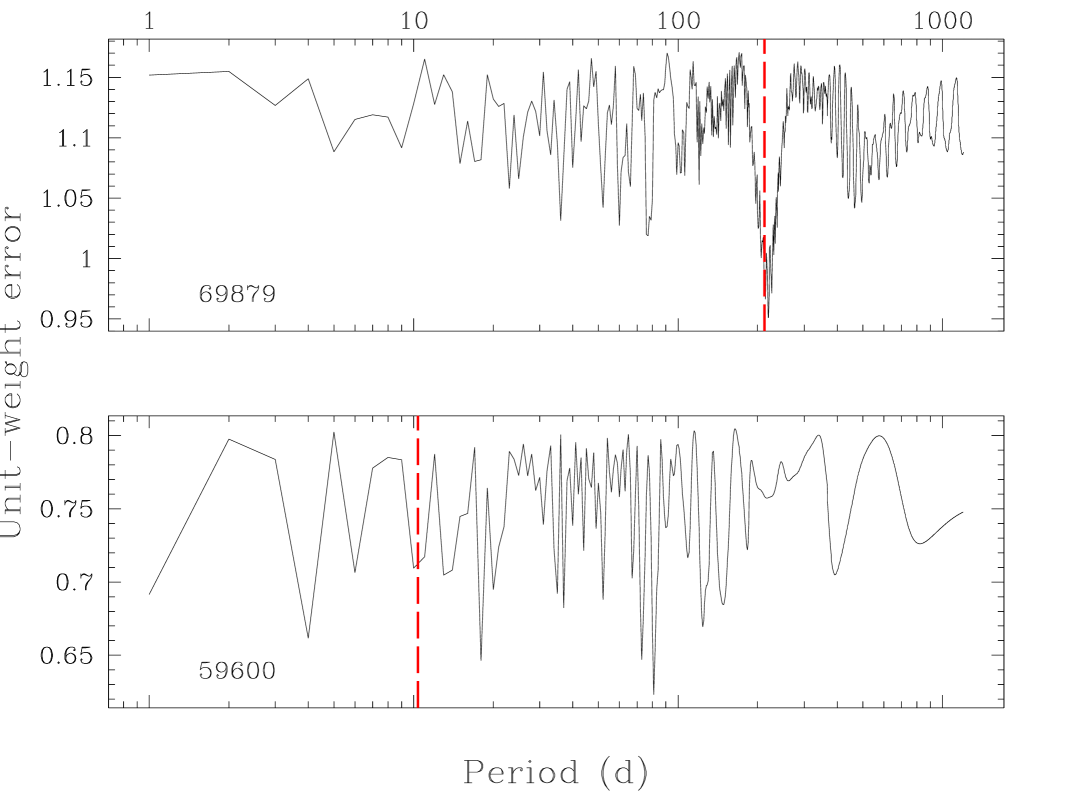
Actually, these tests are based on the fit only and fulfilling them does not mean that what Hipparcos saw is the companion we are interested in and for which we partially adopted an orbital solution. A periodogram can thus be used to see if the IAD do contain a peak at the period corresponding to the spectroscopic one. Two examples are given in Fig. 1. On the one hand, the periodogram of HIP 69879 exhibits a very deep peak at the right location where, on the other hand, the IAD of HIP 59600 do not show any special behavior around 10 days.

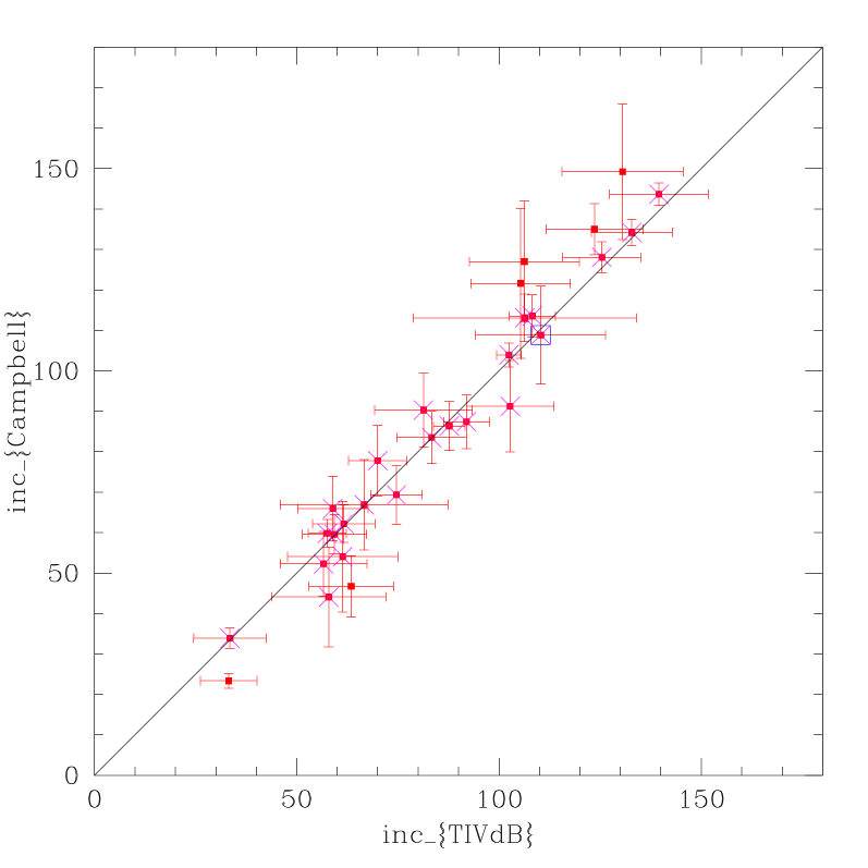
Besides these criteria on the periodicity in the signal and the statistical assessment of the fit, one can also add a criterion based on the correlation among the model parameters (e.g., the efficiency $\epsilon$), say $\epsilon\geq 0.4$ (Eichhorn 1989) and another about a S/N threshold below which no reliable solution is expected, say $a_{0}\sin i\geq 1.5$ mas. Combining all these constraints, one ends up with 29 systems only. The resulting inclinations are plotted in the left panel of Fig. 2. One notices that the systems fulfilling those constraints also have inclinations derived with the two methods in fairly good agreement.

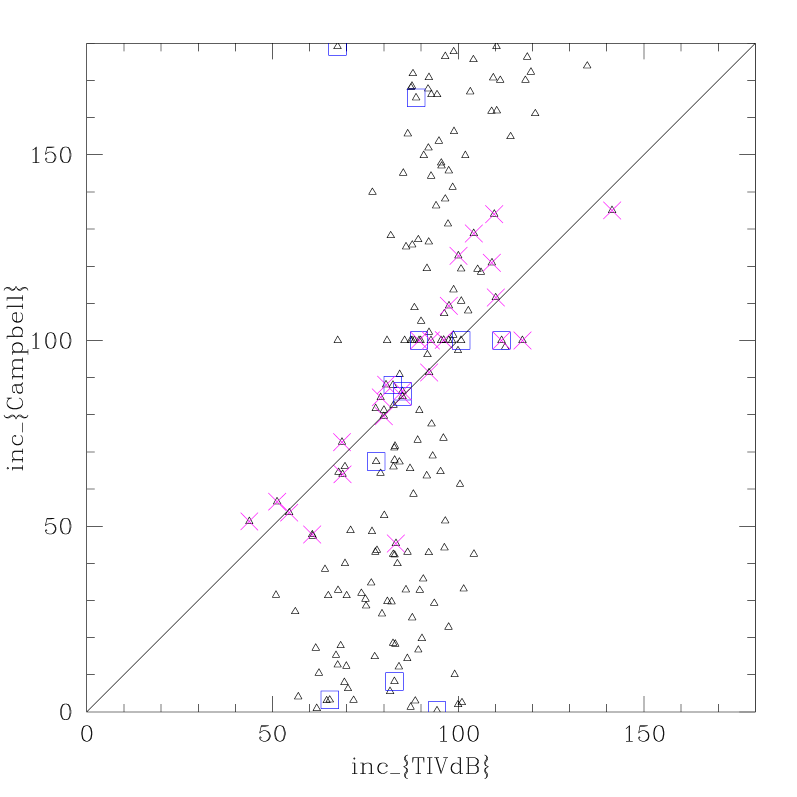
On the other hand, the distribution of the inclinations for the rejected systems is, at first sight, more puzzling. Indeed, the $i$ fitted directly with Campbell’s approach are almost uniformly distributed over $[0,180\degr]$ whereas those resulting from the inversion of the Thiele-Innes constants remain clustered around 90$\degr$. Such clustering is typical of systems where the Thiele-Innes constants are non significantly different from zero as shown by Pourbaix & Arenou (2001) in the context of extra-solar planets. The inclinations derived from Campbell’s method were there always close to 0 or $180\degr$ (whereas they are here uniform over $[0,180\degr]$). However, face-on orbits are not per se the sign of absence of any orbital astrometric signal. Pourbaix (2001) showed that, at low S/N,

$$\sin i\sim\frac{a_{0}\sin i}{\sigma_{\rm IAD}}<a_{0}\sin i$$

the right-hand side of the expression coming from the spectroscopic orbit. In this relation, $a_{0}\sin i$ is the projected angular size of the spectroscopic orbit (the secondary is assumed to be unseen) and $\sigma_{\rm IAD}$ is the standard deviation of the abscissa residuals. Whereas, in case of extra-solar planets, $a_{0}\sin i$ is tiny, it gets very large with spectroscopic binaries (assuming the same units). Therefore, $\sin i$ is no longer constrained to be nearly 0 and $i$ and, thus, can get (uniformly) distributed over $[0,180\degr]$. The right panel of Fig. 2 is thus a perfect illustration of the inclinations derived with the two approaches when there is no astrometric wobble.

Another point worth noting is that a lot of the systems previously processed with an orbital solution (DMSA/O) are no longer kept as such. This is also true for most of the SB2 systems, as all but one had to be discarded. However, these SB2 systems are often rejected because of the small difference of magnitude between the components thus leading to a tiny semi-major axis of the photocentric orbit. On the other hand, about 30% of the systems for which we adopt an orbital solution were initially processed as single stars. It should also be noted that for the majority of the systems we keep and for which an orbital solution (DMSA/O) exists, the orbital elements we derive are generally of much greater accuracy. This makes it useful for the analysis which follows.

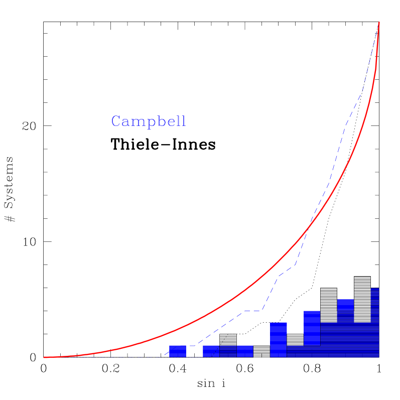
Table 2 gives the inclinations of the 29 accepted orbits and their distribution is given in Fig 3. This distribution is quite consistent with randomly oriented orbits, with just a small excess of nearly edge-on orbits which is an expected observational bias for spectroscopic binaries. Even if the Hipparcos observations are quite precise and accurate, the average precision on these inclination is about 8°. With a behavior in $\sin i$, the consequence of such an uncertainty on the derived mass becomes more important the closer one gets to face-on orbits. For example, even if for the system HIP 8922, the one-sigma error on the inclination is below two degrees, the resulting error on the mass function is larger than 20%. And sometimes, the error on the mass function can become larger than 50%. For a few systems, however, mostly these with an inclination close to 90$\degr$, the error on the mass function can be of the order of 2%. As for these systems, we have generally also a very accurate parallax, the physical parameters we can derive will prove very significant. It is noteworthy that five systems have inclinations close to 90$\degr$, hence which could show eclipses (Table 3). As the companion is supposedly a main sequence star and the separations are rather large, the conditions for eclipses to occur are stringent and the eventual eclipses will be very partial, i.e. very weak. It may in fact be more appropraite to talk of transits. The systems being however very bright, even the small change in luminosity such eclipse would produce should easily be observable by a careful amateur astronomer. Because of the error on the orbital period, it is however not possible to predict with any reliability the time of conjonction.

Table 2: Inclination of the orbits of the 29 kept systems

HIP	$i$ (°)	HIP	$i$ (°)	HIP	$i$ (°)
443	$44\pm 12$	52085	$128\pm 3.8$	87428	$149\pm 17$
2170	$47\pm 7.6$	54632	$122\pm 18$	90659	$144\pm 2.8$
8833	$69\pm 7.2$	57791	$86\pm 6.1$	91751	$60\pm 4.8$
8922	$23\pm 1.8$	59459	$54\pm 14$	92512	$91\pm 11$
10340	$127\pm 15$	59856	$113\pm 5.9$	92818	$52\pm 8.0$
10366	$104\pm 2.9$	61724	$84\pm 6.4$	93244	$87\pm 6.6$
10514	$67\pm 11$	65417	$62\pm 4.6$	95066	$78\pm 8.7$
16369	$66\pm 8.0$	69112	$134\pm 3.2$	103519	$34\pm 2.5$
30501	$109\pm 12$	69879	$90\pm 9.2$	114421	$114\pm 5.3$
46893	$135\pm 6.3$	83575	$60\pm 3.4$

Figure 3: Distribution of the inclinations derived with the two methods. The grey (black) histogram gives the number of inclinations in bins of 0.05 obtained with Campbell’s (Thiele-Innes’) method. The dashed (dotted) line are the corresponding cumulative distributions whereas the solid line represents the distribution if the orbits are randomly oriented. The small excess of nearly edge-on orbits results from a selection effect.

Table 3: Tentative characteristics of the primary eclipses for the systems where $i=90\degr$ is likely. Conjunction times are not given because their uncertainty are of the order of the orbital period.

HIP	Orbital Period	Duration	$\Delta m$
	(d)	(d)	(mmag)
57791	486.7	4.3	11
61724	972.4	5.3	9
69879	212.085	3.7	9
92512	138.42	5.7	4
93244	1270.0	7.0	3

2.2 DMSA/O entries

Table 4: Statistical results (Pourbaix & Arenou 2001) for the rejected DMSA/O entries: Pr₁=Pr($\hat{F_{C}}>F(2,N-7)$), Pr₂=Pr($\hat{F}>F(4,N-9)$); Pr₃=Pr($\chi^{2}_{4S}>\chi^{2}(4)$); Pr₄=Pr($\chi^{2}_{4C}>\chi^{2}(4)$); $\epsilon$ is the efficiency (Eichhorn 1989); The Campbell approach may be accepted when the conditions Pr${}_{1}<5\%$, Pr${}_{2}<5\%$, Pr${}_{3}<5\%$, $|D|<\approx 2$, $\epsilon\geq 0.4$, Pr${}_{4}>5\%$, Pr${}_{5}>5\%$, and $a_{0}\sin i>1.5$ mas are fulfilled.

HIP	Pr1	Pr2	Pr3	$D$	$\epsilon$	Pr4	Pr5	Period	$a_{0}\sin i$	Fitted
HIP								(d)	(mas)	in DMSA/O
10324	15	21	18	-0.42	0.28	74	41	1642.1	7.87	$a_{0},i,\Omega$
13531	59	3	25	+0.47	0.07	16	13	1515.6	22.55	$a_{0}$
14328	34	0	0	-3.51	0.33	0	0	5329.8	47.49	$a_{0}$
17440	0	0	0	-1.98	0.33	0	0	1911.5	29.39	$a_{0},i,\Omega,T$
17932	0	0	0	+3.97	0.68	0	0	962.8	12.29	$a_{0},i,\Omega$
24608	99	53	1	-9.25	0.81	0	0	104.0	19.00	$a_{0}$
24727	0	0	0	+0.25	0.51	0	1	434.8	7.91	$a_{0},i,\Omega,T$
26001	0	0	0	-1.91	0.80	5	1	180.9	4.47	$a_{0},i,\Omega,T$
29982	0	0	0	+0.17	0.29	99	98	1325.0	11.15	$a_{0},i,\Omega$
32578	0	1	5	+0.56	0.19	98	89	1760.9	5.13	$a_{0},i,\Omega$
32768	0	0	0	+5.48	0.75	0	0	1066.0	7.09	$a_{0},i,\Omega,T$
36377	0	0	0	-2.74	0.94	0	0	257.8	7.69	$a_{0},i,\Omega,T$
40326	0	0	0	-0.12	0.82	0	0	930.0	8.31	$a_{0},i,\Omega,T$
45527	99	0	0	+5.88	0.63	0	0	922.0	8.84	$a_{0},i,\Omega,T$
49841	0	0	0	-0.20	0.24	0	0	1585.8	15.18	$a_{0},i,\Omega,T$
53240	0	0	0	-2.00	0.46	4	0	1166.0	5.66	$a_{0},i,\Omega$
57565	27	39	50	-0.87	0.68	91	65	71.7	2.78	$a_{0}$
63613	99	0	0	-12.66	0.73	0	0	847.0	19.17	$a_{0},i,\omega,\Omega,e,P,T$
67234	0	0	0	+1.02	0.84	0	0	437.0	6.31	$a_{0},i,\Omega,T$
80166	1	0	5	-0.86	0.46	83	57	922.8	1.91	$a_{0},i,\Omega$
80816	0	0	0	-0.24	0.57	0	0	410.6	8.65	$a_{0},i,\Omega,T$
85749	0	0	0	+0.59	0.61	1	12	418.2	5.81	$a_{0},i,\Omega$
96683	99	0	5	-0.75	0.71	0	0	434.1	11.59	$a_{0}$
110130	0	0	0	-0.82	0.13	0	0	4197.7	42.38	$a_{0},T$
112158	0	0	0	-3.81	0.81	0	0	818.0	15.55	$a_{0},i,\Omega,T$

As already stated, a lot of the DMSA/O entries (i.e. objects whose observations were initially fitted with an orbital model) get rejected although the inclinations derived with the two methods agree very well (right panel of Fig. 2). Table 2 is therefore likely to be (too) conservative and some further investigation of the DMSA/O entries seems worth undertaking.

The 25 DMSA/O entries rejected (Table 4) can be subdivided into cases where the spectroscopic constraints have to be slightly relaxed on the one hand and those where there is no noticeable and/or reliable improvement with the orbital model on the other hand. For about 50% of these systems, $T$ (the periastron time), though known a priori, was adjusted also. For none of the latter, the orbit is circular. One can therefore wonder how reliable this approach is. Indeed, even if $T$ is not well estimated from the spectroscopic orbit, neither does $\omega$ (the argument of the periastron). It therefore does not make much sense to change $T$ without also fitting $\omega$.

For 19 systems among the rejected ones, either $Pr_{4}$ or $Pr_{5}$ (but usually both) is very close to 0 although the periodogram exhibits a peak at the expected period. $Pr_{4}\approx 0$ indicates that, even if both Campbell’s (14 cases) and Thiele-Innes’ (18 cases) solutions do improve the fit, they do not agree with each other. In order to assess the reliability of the spectroscopic orbit assumed in the fit, that orbit is tested against the CORAVEL radial velocities (S. Udry, private communication) obtained in the framework of the measurement of the whole Hipparcos catalogue with CORAVEL (Fig. 4). Some of the adopted orbits are obviously disproved by those modern radial velocities.

Figure 4: Comparison of the adopted orbits with the CORAVEL data and the quality flag from Batten et al. (1989), ranging from e: ‘very poor and unreliable orbit’ to b: ‘good orbit, but not definitive’. From left to right, the systems are: HIP 24727 (d), 26001 (b), 29982 (b), 49841 (c) (upper panel), 53240 (c), 63613 (e), 67234 (c), and 110130 (c) (lower panel).

2.3 Additional entries

There are six stars for which the orbital model seems appropriate even though they do not belong to the DMSA/O: HIP 2170 (DMSA/C), 8922 (DMSA/X), 10340, 46893 (DMSA/X), 54632, and 87428. The astrometric orbits are given in Table 5.

Table 5: Six new orbital solutions

HIP	2170	8922	10340	46893	54632	87428
$a_{0}$	$6\pm 2.0$	$8.1\pm 0.93$	$3.0\pm 2.6$	$4.8\pm 0.8$	$2\pm 0.55$	$5.3\pm 1.2$
$i$ (°)	$47\pm 7.6$	$24\pm 1.8$	$127\pm 15.0$	$135\pm 6.3$	$122\pm 18$	$149\pm 17$
$\omega_{1}$ (°)	–	–	$358\pm 6$	$261\pm 12$	$332.97\pm 4.23$	–
$\Omega$ (°)	$300\pm 10$	$155\pm 4.0$	$6\pm 17$	$5\pm 11$	$254\pm 22$	$163\pm 15$
$e$	0	0	$0.34\pm 0.03$	$0.149\pm 0.030$	$0.282\pm 0.017$	0
$P$ (d)	$936\pm 4$	$838\pm 4$	$748.2\pm 0.4$	$830.4\pm 2.5$	$18.8922\pm 0.0061$	$467.2\pm 1.2$
$T$ (HJD) (2.4E6+)	$42531.4\pm 2.6$	$43521\pm 5$	$37886\pm 11$	$43119\pm 25$	$23154.071\pm 0.178$	$42484.9\pm 2.7$
Ref	Griffin (1979)	Griffin (1981b)	Griffin & Herbig (1981)	Griffin (1981a)	Sanford (1924)	Griffin (1980)

The case of HIP 2170 is worth mentioning. On the one hand, the companion responsible for the DMSA/C entry was first ever detected by Hipparcos and no ground-based observation has so far confirmed the presence of that companion. On the other hand, the periodogram does exhibit its deepest peak at the spectroscopic orbital period. So it is likely that what Hipparcos saw is actually that spectroscopic companion. With the orbital solution instead of the DMSA/C one, the parallax changes from $1.61\pm 1.24$ mas to $3.65\pm 0.94$ mas, yielding $M_{V}\sim 1$ (instead of -0.76).

2.4 Biases

The BCP93 sample of spectroscopic binaries containing a red giant and its present extension clearly suffer from many observational biases: it is by no means complete in magnitude, it is restricted globally to systems with large enough radial velocity semi-amplitude (i.e. small mass ratios and/or long periods are underrepresented), restricted by definition in the mass range of the primary but not necessarily in the binary population, age, etc. Trying to correct for these biases is a rather challenging task, well beyond the scope of this paper, and one should thus be aware that the results we derive should not be taken as such for the study of binary star formation for example. Already the fact that we are looking only at red giant primaries implies that one should correct everything for the stellar evolution effects. However, as was already the case for BCP93, the idea here is not to obtain directly useful hints on the way stars do form but instead to study the properties of a sample which can be used as a comparison for Peculiar Red Giant stars, and hence which suffers from similar biases. The subsample of 29 orbits that we have selected will clearly suffer at least from the same biases. We have however checked that except for the orbital period, there is statistically no difference between our subsample and the full sample of 215 stars, regarding for example the visual magnitude, mass function or eccentricity distributions. As far as the orbital period is concerned, our subsample is strongly peaked (see Fig. 5) in the period interval between 400 and 1400 days, with the smallest period being about 19 days and the longest 1672 days. There is no obvious reason however why this selection in period should impose a bias on the masses of the two components (but see below) and we may therefore believe that our subsequent analysis is representative of the whole sample of red giant SBs. One should note that the system with the shortest period (19 d) has in fact a main-sequence primary (see below).

Figure 5: Distribution of the logarithm of the orbital period for the full sample and for our selected subsample of 29 systems (shaded area). The subsample shows a strong peak for systems between 400 and 1400 days,

3 Mass function and masses of the primary

With the knowledge of the inclination as given by Table 2, we can estimate for each of the 29 systems, from the mass function $f(m)$, the quantity denoted by $\cal{Q}$ in BCP93, and which is a function of the masses of the two components ($m_{1}$ & $m_{2}$) of the binary system:

$${\cal Q}=\frac{f(m)}{\sin^{3}i}=\frac{m_{2}^{3}}{(m_{1}+m_{2})^{2}}.$$ (1)

Figure 6: Distribution of the logarithm of $\cal{Q}$ for the sample of 28 single-lined systems which we retained. The error bars correspond to a Monte Carlo estimate taking into account the errors on $\cal{Q}$. The dashed curve is a Gaussian fit to the data, with a mean at -1.08 and a half width at half maximum of 0.45.

The resulting distribution of the logarithm of this quantity is shown in Fig. 6. It can be seen that the distribution is compatible with a Gaussian with a mean at -1.08 and a sigma of 0.45. Such a mean value corresponds to a mass of a companion of 0.7, 0.9 and 1.1 M_⊙ for a primary mass of 1.5, 2 and 3 M_⊙, respectively. There is a small excess of systems having $\log$ $\cal{Q}$ around -1.75. This value of $\cal{Q}$ corresponds to a mass of a companion of 0.4, 0.5 and 0.6 M_⊙ for the above quoted value of the primary mass.

We have also performed a comparison between the distribution of $\cal{Q}$ one would obtain assuming a random inclination, both for our subsample of 28 systems and for the full sample of 215 systems. A Kolmogorov-Smirnov test could not distinguish between the two derived distributions. This confirm that our subsample should be statistically representative of the full sample of red giants spectroscopic binaries.

In the case of single-lined spectroscopic binaries, and even when one knows the inclination of the system, there is no immediate way to determine the mass of the components, not even for the primary. In our case, as the systems have red giant primaries, it is also not possible to make use of a simple mass-luminosity relation to estimate the mass as would be the case - as a first approach - for main-sequence stars. If sufficiently accurate information is available, however, on the effective temperature - either through spectroscopy or from the colors - and on the bolometric luminosity - through a good knowledge of their parallax - one can hope to estimate a reasonable mass of the primary by using an Hertzsprung-Russel diagram and compare with stellar evolutionary tracks. As the 29 stars we have selected were, by definition, observed by Hipparcos and reanalyzed by us, a good estimate of the parallax and its associated error is available. The stars being bright, good values of their magnitude and $(B-V)$ color index are available. Moreover, McWilliam (1990) has produced a high-resolution spectroscopic survey of 671 G and K field giants which includes most of them. This allows to have a good determination of the effective temperature as well as of the metallicity of our stars. Most of our stars have solar metallicity, with the most metal-poor star being HIP 90659 with a [Fe/H]=-0.67.

We have thus obtained for the 29 stars in our significant sample the bolometric magnitude ($M_{\rm bol}$) and the effective temperature ($T_{\rm eff}$). For $T_{\rm eff}$, we searched for values in the literature, with most values being obtained from McWilliam (1990). If no value was found, we estimated one from the $(B-V)$ index using the relation (McWilliam 1990) :

$$T_{\rm eff}=8351-4936\leavevmode\nobreak\ (B-V)+1456\leavevmode\nobreak\ (B-V)^{2}-78\leavevmode\nobreak\ (B-V)^{3}.$$ (2)

The bolometric magnitude was obtained from the parallax ($\varpi$, in mas) and bolometric correction ($BC$), through the relations :

$$M_{\rm bol}=m_{V}-5\leavevmode\nobreak\ log\frac{1000}{\varpi}+5-A_{V}+BC,$$ (3)

where $A_{V}$ is the visual extinction given by version 2.0.5 of the EXTINCT subroutine (Hakkila et al. 1997). The value of $BC$ was estimated from $T_{\rm eff}$ using the tables of Lang (1992).

The results are shown in Fig. 7, where for clarity we have separated our sample into 4 arbitrary sub-samples. One sigma errors are also indicated. On these figures, we also show the evolutionary tracks for stars of solar metallicity with masses between 0.8 and 5 M_⊙ as obtained by the Geneva group (Schaller et al. 1992; Charbonel et al. 1996). From the comparison of the positions of these stars and their uncertainties, one can estimate the probable range of mass of the primary of each system. One has to note that because these systems are single-lined spectroscopic binaries, the secondary should not contribute too much light to the whole system, Hence, using the total luminosity of the system and color of the system to derive the mass of the primary should not be a large source of error. This will be checked a posteriori (see Sect. 4). As all the systems for which the metallicity is known have close to solar abundance, we do not need to compare our data with stellar evolutionary tracks corresponding to other value for Z than 0.02. All our results are summarized in Table 6 where we indicate, respectively, the HIP identification number, the effective temperature, the parallax and its sigma deviation, the bolometric magnitude, the mass of the primary, the lower and upper limits on the mass of the primary, the mass of the secondary, and the mass ratio.

Figure 7: Position of the retained 28 single-lined systems in the H-R diagram. For comparison, we show the stellar evolutionary tracks for Z=0.02 stars as obtained by the Geneva group. The curves are labeled with the initial stellar mass on the main sequence, in solar masses.

The distribution of primary masses are shown in Fig. 8. It is strongly peaked around 2 M_⊙ with only 3 out of 28 systems having a primary mass equal or above 3 M_⊙. A value of 2 M_⊙ is consistent with the results of Strassmeier et al. (1988) who obtain the same value for the red giant component of binary systems. More recently, Zhao et al. (2001) also concluded that the majority of red clump giants have masses around 2 M_⊙. BCP93 favored a mass of the red giant primary of 1.5 M_⊙ in their statistical analysis, while Trimble (1990) assumed a mass of 3 M_⊙. From our analysis, this last value seems too large, while the first appears slightly too small.

4 Masses of secondary and mass ratio distribution

With the value of the primary mass deduced from the H-R diagram and the value of the quantity $\cal{Q}$ deduced from the inclination and the mass function, one can now determine for each system the mass ratio and the secondary mass. This is a straightforward exercise which only requires to solve a third degree polynomial. The values for the individual masses will be discussed later (see Sect. 7). Here we will look at the distribution of these quantities so as to compare with the previous analysis of BCP93 and others.

Figure 8: Distribution of the masses of the primary for the 28 single-lined SBs. The solid line shows the distribution taking the face value of the primary masses, while the dashed line shows the distribution with the possible range for each primary mass as derived from the one sigma errors shown in the HR diagram.

Figure 9: Distribution of the masses of the secondary for the 28 single-lined SBs.

Figure 10: Distribution of the mass ratio for the 28 single-lined SBs.

The distribution of the secondary mass ($m_{2}$) is shown in Fig. 9. It appears to be exponentially increasing for smaller masses with a drop-off for secondary masses below 0.5 M_⊙. This drop-off must be related to the absence of systems in our sample with a mass ratio below 0.2 (see below). We have checked that the distribution of $m_{2}$ can be fitted with a Salpeter-like IMF with $\alpha=2.35$ when for each system $m_{2}$ is restricted in the range from 0.55 M_⊙ to $m_{1}$. The upper limit is straighforward as we are dealing with red giant primaries and the companion must be either less evolved and hence less massive, or must be a white dwarf and therefore less massive than the giant whose mass is generally above 1.4 M_⊙. The lower limit can be derived from the fact that our subsample contains mostly systems for which the orbital period is larger than 400 days, the radial velocity semi-amplitude is larger than 10 kms^-1 and the mass of the primary is larger than 1.4 M_⊙. From the definition of the mass function, this provides a lower limit to the mass of the secondary. This is a clear observational bias against low mass secondaries but should not question the validity of the apparent IMF distribution of secondary masses.

The median of the distribution is around 0.8 M_⊙ with the largest peak around 0.75 M_⊙, even though there is also a small clustering around 0.52 M_⊙. There are 4 systems - excluding the double-lined spectroscopic binary (see below) - with a secondary mass above 1.5 M_⊙. One should be careful however that these systems might be masqueraders, as in the largest systems, the secondary might well be itself a close binary. This is a scenario which seems very probable for HIP 65417 which has a secondary mass of 2.5 M_⊙ for a primary mass of 2.7 M_⊙ in a long period system, 1367 days. In fact, given these values, this systems is the one with the largest semi-major axis, 4 AU. In such a system, it is no problem to have a hierarchical triple system with the secondary being itself a close binary system composed of two F or G main sequence stars with an orbital period of a few tens of days. This was in fact already suggested by Griffin (1986a).

For the other systems, we have checked that there is no apparent correlation between the mass of the secondary and the orbital period (or the semi-major axis) so that there is no reason to believe in having a triple system.

We now turn to the distribution of the mass ratio which is shown in Fig. 10. Two facts are easily seen. First, the distribution clearly increases for smaller mass ratios. Second, there are no system with a mass ratio below 0.2. This second effect is clearly a bias related to the need to find an astrometric signal for the stars we have selected. Such a signal becomes weaker for smaller mass ratios, as in the case where the secondary does not contribute to the light of the system, the motion of the photocenter is given by the motion of the primary, hence:

$$a_{0}\equiv a_{1}=\frac{m_{2}}{m_{1}+m_{2}}a=\frac{q}{1+q}a.$$ (4)

For the most close (on the sky) systems, it is not possible to detect the motion if the mass ratio is too small. And indeed, except for one case, there are no systems with a mass ratio below 0.4 with an angular semi-major axis smaller than 15 mas.

The distribution of mass ratios increasing for smaller mass ratios is thus even stronger than we obtain. One should note that there is no obvious reason why there should be a bias against larger mass ratios. Indeed, except for the case of $q$ very close to 1, resulting in a system with two giants, hence a double-lined binary, a larger $q$ makes the astrometric signature more visible. And from the full catalogue, the number of SB2 is rather limited (see also BCP93).

BCP93 had to assume a constant mass for the red giant primary - or an IMF-type distribution - and found that the mass ratio distribution (MRD) is either compatible with a uniform distribution for $m_{1}=1.5$ M_⊙ but more peaked towards smaller mass ratio for $m_{1}=3$ M_⊙. Heacox (1995) performed an analysis of the same sample as BCP93 and found a MRD peaked at values of the mass ratio between 0.3 and 0.5, with a drop off at smaller values. Using a subsample of K giant primaries, Trimble (1990) derived a $q^{-1}$ MRD but BCP93 have shown that this is in fact an artifact of the method used and does not reflect the true MRD of the sample. The MRD we derive here seems to be even more peaked than $q^{-1}$. To better understand this, we have also derived the MRD from our 28 systems, assuming - as BCP93 and Heacox (1995) - a single value of 1.5 M_⊙ for $m_{1}$. In this case, we obtain a similar MRD as the one obtained by Heacox. The fact that the MRD we obtain here is even more peaked in the range 0.3-0.5 must be related to the non-uniqueness of the mass of the primary and the fact that it is more strongly peaked at 2 M_⊙ instead of 1.5 M_⊙.

We have also tried to see if there was any correlation between the masses of the two components and/or with the mass ratio. There is clearly no correlation between the mass of the primary and the mass ratio. Nor is there any significant relation between the masses of the two components. A clear trend is however seen between the mass of the secondary and the mass ratio. This is illustrated in Fig. 11. This might be a consequence of the strongly peaked value for the primary mass.

Figure 11: Mass ratio vs. the secondary’s mass for the 28 single-lined SBs. A clear trend is visible.

Table 6: Parameters of the 28 single-lined systems we retain

HIP	$T_{\rm eff}$	$\varpi\pm\sigma_{\varpi}$	$M_{\rm bol}$	$m_{1}$	$m_{1}^{\tt inf}$	$m_{1}^{\tt sup}$	$m_{2}\pm\sigma_{m2}$	$q\pm\sigma_{q}$
443	4750	24.7 $\pm$0.98	0.99	1.7	1.3	2.1	0.76$\pm$0.11	0.45$\pm$0.05
2170	4660	3.65 $\pm$0.94	0.41	2.	1.7	2.3	1.8 $\pm$0.2	0.9 $\pm$0.05
8833	4930	18.37$\pm$0.76	0.46	2.3	2.	2.6	0.54$\pm$0.04	0.23$\pm$0.01
8922	4270	9.66 $\pm$0.83	0.45	1.	1.	1.2	0.7 $\pm$0.05	0.62$\pm$0.03
10340	3960	6.0 $\pm$0.74	-2.33	2.	1.7	2.7	0.5 $\pm$0.1	0.25$\pm$0.03
10366	4900	16.15$\pm$0.81	0.88	2.	1.6	2.4	1.12$\pm$0.13	0.56$\pm$0.05
10514	4030	3.19 $\pm$0.82	-2.17	2.	1.5	2.5	1.44$\pm$0.2	0.72$\pm$0.08
16369	4710	8.955$\pm$0.88	-1.59	4.	3.3	4.7	1.13$\pm$0.13	0.28$\pm$0.03
46893	4440	7.72 $\pm$0.90	0.07	1.5	1.2	2.	0.54$\pm$0.1	0.36$\pm$0.04
52085	5000	15.61$\pm$0.77	0.47	2.5	2.1	2.9	0.52$\pm$0.06	0.21$\pm$0.01
54632	5910	22.82$\pm$0.58	3.77	1.15	1.0	1.3	0.85$\pm$0.04	0.74$\pm$0.03
57791	4670	12.67$\pm$1.00	0.62	1.7	1.2	2.2	0.90$\pm$0.17	0.53$\pm$0.07
59459	4740	5.37 $\pm$0.84	-0.13	2.5	2.1	2.9	0.72$\pm$0.07	0.29$\pm$0.02
59856	4500	10.45$\pm$0.91	-0.50	2.	1.7	2.6	0.62$\pm$0.11	0.31$\pm$0.03
61724	4840	11.69$\pm$1.00	0.36	2.3	2.0	2.8	0.82$\pm$0.1	0.36$\pm$0.03
65417	4660	5. $\pm$0.85	-0.60	2.7	2.2	3.2	2.5 $\pm$0.25	0.92$\pm$0.07
69112	4120	6.26 $\pm$0.47	-2.07	2.5	2.	3.	1.74$\pm$0.2	0.7 $\pm$0.06
69879	4730	14.63$\pm$0.68	0.11	2.2	1.9	2.5	0.98$\pm$0.08	0.44$\pm$0.03
83575	4600	9.68 $\pm$0.92	0.43	1.7	1.2	2.2	0.87$\pm$0.16	0.5 $\pm$0.08
87428	4530	9.66 $\pm$1.66	0.46	1.5	1.	2.3	0.74$\pm$0.21	0.5 $\pm$0.08
90659	5150	8.43 $\pm$0.87	2.35	1.6	1.2	2.	0.35$\pm$0.06	0.22$\pm$0.02
91751	4800	13.26$\pm$0.08	1.11	1.7	1.6	1.8	0.71$\pm$0.025	0.42$\pm$0.01
92512	4400	10.28$\pm$0.42	-1.02	2.5	2.	2.8	1.3 $\pm$0.16	0.54$\pm$0.05
92818	5160	6.535$\pm$0.63	-1.67	4.	3.6	4.4	1.88$\pm$0.11	0.47$\pm$0.02
93244	4740	21.74$\pm$0.70	0.09	2.1	1.9	2.5	0.47$\pm$0.05	0.22$\pm$0.01
95066	4940	8.92 $\pm$0.48	-0.80	3.2	3.	3.4	1.4 $\pm$0.05	0.44$\pm$0.01
103519	4920	12.29$\pm$0.63	0.52	2.3	2.	2.6	0.87$\pm$0.07	0.38$\pm$0.02
114421	4800	18.25$\pm$0.78	0.69	2.	1.6	2.4	0.75$\pm$0.1	0.38$\pm$0.03

Figure 12: Position of the two components of the SB2 HIP 30501 in the H.-R. diagram. The curves are the Schaller et al. (1992) evolutionary tracks, labeled with the initial stellar mass on the main sequence.

Figure 13: Radius of the primary of the 28 systems plotted as a function of the logarithm of the orbital period (above) and of the eccentricity (below). The shortest system has a main sequence primary.

5 Radius and luminosity ratio

With the value of the luminosity determined and the effective temperature known, we can estimate the radius of the primary of the 28 SB1 of our sample. We plot in Fig. 13 the radius as a function of the orbital period and of the eccentricity. The first plot clearly shows that the smallest system contains a main-sequence primary. The smallest period in our sample is thus 73 days, but even for this system, it can be seen from the analysis presented in the above sections that the primary is most probably still in the sub-giant phase. This diagram thus clearly shows the fingerprint of stellar evolution. It may also show the effect of binary evolution, as the largest radius are only present in the longer system. Three systems have a zero eccentricity and they all have rather large periods. Unless these systems were formed in a circular orbit, it might well be that, as explained by BCP93, they either contain a white dwarf or they are clump giants which went already through their maximum radius on the first ascent giant branch. Note that because of the large secondary mass we deduce for HIP 8922, it is unlikely to contain a white dwarf.

Once the mass of the secondary has been deduced, and assuming it to be on the main-sequence, one can estimate its luminosity, hence the luminosity ratio between the components. This could then be used in principle to determine the motion of the photocenter and compare it to the value derived from the astrometry. This is hardly useful in practice. Indeed, for most systems, the $a_{0}$ deduced from the astrometric solution has too large an error to be used as an additional constraint on the solution. Moreover, in most cases, the luminosity ratio is so high that the photocenter is at the location of the primary. In a few cases, however, this can be used as a check of the correctness of our analysis. For example, for HIP 8922, we can deduce from our solution that the luminosity ratio is 5.5 10^-3. We can also compute that the semi-major axis is 2 AU, or 19.6 mas. Given the mass ratio of 0.7, we predict a motion of the photocenter of 8.1 mas, exactly the value which comes out from our astrometric solution.

As an example of the other extreme, let us consider HIP 2170. From the value of $i,m_{1},m_{2}$ and $P$, we can deduce a separation about 3 AU, or 11 mas. With the $a_{0}$ from the astrometry ($6\pm 2$ mas) and the value of $m_{2}/(m_{1}+m_{2})=0.47$, it appears that the luminosity ratio must be very small. However, from the value of $m_{2}$, one expects a luminosity ratio of about 20%. Thus, either the secondary is itself a close binary or the error on $a_{0}$ preclude from any conclusion. There is however enough place in this system to have a hierarchical triple with the inner binary having an orbital period of 40 days or less.

A few other examples are discussed individually in Sect. 7.

6 HIP 30501: a SB2 with an astrometric solution

HIP 30501 is the only double-lined spectroscopic binary which was kept from our initial full sample. This is hardly surprising as, for an SB2, the luminosity ratio being close to 1, the photocenter’s motion is very much reduced with respect to the one of the binary components and is therefore very difficult to detect. It is thus quite a surprise to nevertheless still believe that in one case Hipparcos detected the astrometric motion of the photocenter.

HIP30501 is a 577 days binary with a mass ratio of 0.97 (Griffin 1986b). It contains two giants in an $e=0.24$ eccentric orbit. The solution we derive for this system is different, but within the errors bars, from the one listed in the DMSA/O : $i=109\pm 12\degr$ (instead of $121\pm 21\degr$); $a_{0}=4.16\pm 1.28$ mas (instead of $2.92\pm 1.13$ mas; $\varpi=3.36\pm 0.94$ mas (instead of $3.92\pm 0.96$ mas.

With our value of $i$ - or the one of Hipparcos for that matter - no eclipse should unfortunately occur in this system. Using $i$, we derive the masses of the two components: $m_{1}=3.10\pm 0.65$ M_⊙ and $m_{2}=3.02\pm 0.64$ M_⊙.

Griffin (1986b) estimates the difference in magnitude as $1.24\pm 0.10$ mag if the two components have the same spectral type. It is this difference in magnitude which explains why Hipparcos could detect the motion of the photocenter. Would the two stars have been closer in their luminosity, the detection would have proven impossible. The relatively large uncertainty on $a_{0}$, $\sin i$ and $\varpi$ makes it unfortunately not possible to use the value of $a_{0}$ to constraint the luminosity ratio.

A note of caution is here required. If the 1.24 mag difference is real then, because the mass of the two stars are very close and because they are on the steep slope of the giant branch in the H-R diagram, they cannot in fact have the same effective temperature! And therefore one cannot believe the 1.24 mag estimate. In reality, there is a range of solution possible, which is limited by the fact that the integrated $(B-V)$ index be equal to 1.21 and by the value of the absolute visual magnitude of the whole system. This allows the primary to be of spectral type K2-K3 III, while the secondary would be of type K0-K1 III. The difference in magnitude ranges from 0 (if both star have the same spectral type, a rather unlikely situation has they have different masses but the same age) to about 1.4 (when the primary would become too cool and too bright to fulfill the constraints). These parameters imply an age of roughly $4.\leavevmode\nobreak\ 10^{8}$ years, based on the Schaller et al. (1992) evolutionary tracks. We show one of the possible solution in Fig. 12.

It has to be noted that 3 of our 28 single-lined spectroscopic binaries might in fact be double-lined as the estimate of their difference in magnitude is about 1.1-1.3 if one assumes the companion is a main-sequence star of mass $m_{2}$. These three stars are HIP 2170, 54632 and 65417. The fact that there were not detected as SB2 yet might be due to observations done at too low resolution (e.g. HIP 54632), with a radial-velocity spectroscopy not sensible enough to A-F type star (e.g. HIP 2170) or that the companion itself is a close binary (e.g. HIP 65417). Further studies of these stars are thus called for.

7 Individual cases

In this section, we now look in turn to each individual cases.

HIP 443: This is a RS CVn star with an orbital period below 73 days. It is rather surprising that Hipparcos could detect the astrometric signature of this system, but this is certainly due to the relatively large value of the parallax. Although the DMSA/O solution quoted a value of $36\pm 37\degr$ (!) for the inclination, our reanalysis shows a more secure value of $44\pm 12\degr$. The secondary is constrained to be a low mass star, in the range 0.5 to 1 M_⊙. Although there were several attempts, this system has never been resolved by (speckle) interferometry (Hartkopf et al. 2001).

HIP 2170: One of the systems with a rather large mass ratio, between 0.8 and 1. The parallax we deduce is sensibly different from the one in the Hipparcos catalogue (3.65 vs. 1.61).

HIP 8833: We obtain a slightly larger value of the parallax than the Hipparcos DMSA/O solution and a more accurate orbital solution. Zhao et al. (2001) quote a value of 2.5 M_⊙ for the mass of the giant, in good agreement with our $2.3\pm 0.3$ M_⊙ value. The mass ratio is well constrained to lie around 0.23, leading to a companion mass of 0.55 M_⊙. No enhancement of s-process elements was detected by McWilliam (1990). Although there were several attempts, this system has never been resolved by (speckle) interferometry (Hartkopf et al. 2001).

HIP 8922: Although this system has an orbital period of 838 days, Hipparcos did not find an orbital solution. Our reanalysis however provides a very precise value for the inclination, $23\pm 2\degr$. With such a large period, a null eccentricity and a very small mass function, this star belongs to the class of stars defined by BCP93 to possibly harbor a white dwarf. The value for the secondary mass, $0.7\pm 0.05$ M_⊙ is certainly not an argument against. Unfortunately, no abundance analysis has been published for this star so that we cannot check if it belongs to the class of PRGs. Although there were several attempts, this system has never been resolved by (speckle) interferometry (Hartkopf et al. 2001).

HIP 10340: Another long period, low mass function system. The range in mass for the secondary does also allow a degenerate companion. For this star, however, stellar abundance show it not to be enriched in s-process elements (Jorissen & Boffin 1992; McWilliam 1990) even though it is sometimes referred as Ba0.5. It might thus represent an example of the fact that binarity is not a sufficient condition for the barium star phenomenon. It has however been claimed that this system was resolved by speckle interferometry (McAlister et al. 1987) even if only two measurements are available (Hartkopf et al. 2001). With the parameters we derive, such a detection is questionable.

HIP 10366: We derive a very accurate solution for this very eccentric orbit ($e=0.8815$) and deduce a 2 M_⊙ mass for the giant and a 1.1 M_⊙ for its companion. This star is among the normal stars in the sample of McWilliam (1990). Our solution leads to a semi-major axis of 3.87 AU or 62.6 mas, and taking the face values of the components masses, a value of $a_{1}=22.5$ mas in perfect agreement with the value obtained from spectroscopy. This is close to the $a_{0}$ value derived from astrometry, even though it is a little too large, especially if one has to take into account the fact that it is photocentric motion and not the motion from the giant that we see. Balega et al. (1984) once resolved this system by speckle interferometry.

HIP 16369: One of the most massive giant in our sample, with a primary mass of $4\pm 0.7$ M_⊙ and a companion with a mass close to 1 M_⊙. Although the DMSA/O solution quotes a value of the inclination of $37\pm 29\degr$, our reanalysis provides a very different but well determined value of $66\pm 8\degr$. Although there were several attempts, this system has never been resolved by (speckle) interferometry (Hartkopf et al. 2001).

HIP 46893: This star was in the DMSA/X annex of the Hipparcos catalogue which could not find an orbital solution. Our analysis provides it with a very similar but more accurate parallax. Although there were several attempts, this system has never been resolved by (speckle) interferometry (Hartkopf et al. 2001).

HIP 52085: The parallax we obtain is slightly larger than the one in the Hipparcos catalogue. Our orbital solution also is different from the one in the DMSA/O with an inclination of $128\pm 4\degr$ instead of $147\pm 12\degr$. McWilliam (1990) does not detect any s-process enhancement in this star. Although there were several attempts, this system has never been resolved by (speckle) interferometry (Hartkopf et al. 2001).

HIP 54632: The shortest orbital period in our sample, 19 days, and identified as single in the Hipparcos catalogue. This is clearly a main-sequence star of spectral type G0 V and a mass of $1.15\pm 0.1$ M_⊙. The mass ratio is in the range 0.5 to 0.9, even though the largest value must not be the correct one as the system would appear as an SB2 in this case.

HIP 57791: One of the few example where our solution is similar to the one given in the DMSA/O annex. With an inclination of $86\pm 6\degr$, this system could be eclipsing. The rather secure mass ratio we derive is $0.53\pm 0.07$. This system is resolved by speckle interferometry (McAlister et al. 1983) but only three measurements have ever been obtained (Hartkopf et al. 2001).

HIP 59459: No luminosity class exist for this object but our analysis shows it to be a giant albeit slightly hotter than the K2 spectral type mentioned in the Simbad database.

HIP 59856: McWilliam (1990) does not detect s-process enhancement in this star for which we obtain a companion mass around 0.6 M_⊙ and a mass ratio close to 0.31. Our solution is more accurate and in better agreement with the spectroscopic one than the Hipparcos DMSA/O one. Although there were several attempts, this system has never been resolved by (speckle) interferometry (Hartkopf et al. 2001).

HIP 61724: Another case of a possible eclipsing system and a solution in agreement with the one quoted in the DMSA/O. Although there were several attempts, this system has never been resolved by (speckle) interferometry (Hartkopf et al. 2001).

HIP 65417: This is the binary with the larger mass ratio we found, $q=0.92\pm 0.07$. Assuming a main sequence companion, the difference in visual magnitude could therefore only be slightly larger than 1 magnitude (but see Sect. 4.). The star was observed by Začs et al. (1997) has having no s-process enrichment, which is no surprise if as we estimate the companion must have a mass above 2 solar masses. Although there were several attempts, this system has never been resolved by (speckle) interferometry (Hartkopf et al. 2001).

HIP 69112: We find a giant mass of $2.5\pm 0.5$ M_⊙ and a mass ratio around 0.7. The companion, with a mass close to 1.7 M_⊙, if on the main-sequence, must be of spectral class A7 V. Unpublished IUE observations of this star (Boffin 1993) show indeed the presence of a late A-early F companion. Richichi & Percheron (2002) quote an angular diameter for the giant of 2.76 mas. With our adopted solution, we found a value of 80 solar radii, or 2.41 mas, close to the above-mentioned value. Bonneau et al. (1986) resolved this system but other attempts remained unsuccessful (Hartkopf et al. 2001).

HIP 69879: This is certainly, with an inclination of $90\pm 9\degr$, one of the best candidate of an eclipsing system. The solution we found is also well constrained with a primary mass of $2.2\pm 0.3$ M_⊙ and a mass ratio of $0.44\pm 0.03$. Taking the parameters of the K0 III giant, i.e. a radius of 12.3 R_⊙ and assuming a one solar mass companion, one obtain an eclipse depth of 9 mmag. In the Hipparcos catalogue, HIP 69879 is classified as a new variable with an amplitude of 17 mmag. However, we have checked that no periodicity appear in the Hipparcos data and the variability detected is therefore not consistent with the assumption of an eclipse. Although there were several attempts, this system has never been resolved by (speckle) interferometry (Hartkopf et al. 2001).

HIP 83575: Our solution for this star is similar, but more accurate, than the one quoted in the DMSA/O. The mass ratio is very close to 0.5. Although there were several attempts, this system has never been resolved by (speckle) interferometry (Hartkopf et al. 2001).

HIP 87428: Noted as single in the DMSA/O, the solution we obtain is not very useful as the uncertainty on the mass function is of 100 %.

HIP 90659: A G8 III-IV which is indeed verified by our solution, not very different from the DMSA/O one. Začs et al. (1997) do not detect any s-process enhancement and our analysis show that the companion is most probably a low mass star, in the range 0.3-0.4 M_⊙. This is too small a value for a white dwarf.

HIP 91751: Here again, our solution is close to the DMSA/O but slightly more accurate. The mass ratio of this system is well constrained in the $0.42\pm 0.03$ range. Although there were several attempts, this system has never been resolved by (speckle) interferometry (Hartkopf et al. 2001).

HIP 92512: Another potential eclipsing system, also quoted as variable in the Hipparcos catalogue with an amplitude of 0.04 mag. With its rather short period of 138.7 days, it is however of the RS CVn type which could be the cause of the variability. Our solution implies a 1.3 M_⊙ companion and a 2.5 M_⊙ primary. An eclipse should have an amplitude of about 3-4 mmag only. Although there were several attempts, this system has never been resolved by (speckle) interferometry (Hartkopf et al. 2001).

HIP 92818: The second 4 solar mass giant in our sample with a mass ratio slightly below 0.5. With our solution, we derive a radius for the G4 III giant of 24 R_⊙ or 0.73 mas. This is in very good agreement with Blackwell et al. (1991) who found an angular diameter of 1.4 mas. Hummel et al. (1995) found a A6V companion with a difference of 2 magnitudes between the components. This is also in very good agreement with the 1.9 M_⊙ we derive for the companion, even though we predict a 3.4 mag difference in V.

HIP 93244: Another possible eclipsing system, with an inclination of $87\pm 7\degr$. Our solution, close to the DMSA/O one, gives a radius of 12 R_⊙ (1.2 mas) for the 2 M_⊙ giant, in perfect agreement with the value obtained by Nordgren et al. (1999). The companion should have a mass between 0.4 and 0.5 M_⊙ and an eclipse would therefore only show a dip of 2-3 mmag. Although this star has been sometimes referred as a Ba0.2 star, McWilliam (1990) found a normal s-process abundance and we guess that the companion is a normal low-mass star. With such a small companion, the difference in magnitude between the two components should be more than 7 magnitudes, and the photocentric motion can therefore very well be approximated by the motion of the giant star. In this case, taking the face value of the masses we derived, we obtain a semi-major axis of 3.14 AU or 68 mas. The value of $a_{1}$ is therefore about 12.5 mas, in very good agreement with the value deduced from the $a_{1}\sin i$ value deduced from spectroscopy and the $a_{0}$ one deduced from the astrometric solution. We are thus confident about the accuracy of our model.

HIP 95066: Although there were several attempts, this system has been resolved only twice by (speckle) interferometry (Hartkopf et al. 2001).

HIP 103519: Our solution is very similar to the DMSA/O one. McWilliam (1990) did not detect any enhancement of s-process elements in this giant. We derive a mass of the companion close to 0.9 M_⊙ for a mass ratio around 0.38. Although there were several attempts, this system has never been resolved by (speckle) interferometry (Hartkopf et al. 2001).

HIP 114421: We obtain a slightly larger value of the parallax than the Hipparcos DMSA/O solution. The mass ratio is here also around 0.38. Although there were several attempts, this system has never been resolved by (speckle) interferometry (Hartkopf et al. 2001).

8 Conclusion

We have updated the catalogue of spectroscopic binaries containing a red giant of Boffin et al. (1993) and cross-identified it with the Hipparcos catalogue. A sample of 215 systems was obtained. For these, we have reanalyzed their Hipparcos Intermediate Astrometric Data and applied new statistical tests which combine the requirement for the consistency between the Thiele-Innes and the Campbell solution as proposed by Pourbaix & Arenou (2001) with the requirement that the most significant peak in the Hipparcos periodogram corresponds to the orbital period. By doing so, we select 29 systems among which one double-lined spectroscopic binary, for which we are confident the newly derived astrometric solution is consistent with the spectroscopic orbit. Among these, 6 are new orbital solutions not present in the DMSA/O catalogue. On the other hand, our procedure has rejected 25 DMSA/O entries. For some of these, new radial velocities are indeed in contradiction with the DMSA/O orbits, confirming our rejection.

Our sample of 29 systems allows to derive the distributions of the masses of the components as well as the mass ratio distribution. We find that the mass of the primary is peaked around 2 M_⊙, that the secondary mass distribution is consistent with a Salpeter-like IMF and that the mass ratio distribution rises for smaller value of the mass ratio.

The only double-lined binary in our sample is HIP 30501 for which we find that the primary must be of spectral type K2-K3 III, while the secondary would be of type K0-K1 III. Three other systems should be more closely studied (HIP 2170, 54632 and 65417) as our solution make them potential double-lined systems.

Finally, we find that five systems might have inclination close to 90 degrees (HIP 57791, 61724, 69879, 92512 and 93244) and could therefore possibly show eclipses. The depth of which will typically be of the order of 0.01 mag or below.