Sub-au imaging of water vapour clouds around four Asymptotic Giant Branch stars

Abstract

We present MERLIN maps of the 22-GHz H₂O masers around four low-mass late-type stars (IK Tau U Ori, RT Vir and U Her), made with an angular resolution of $\sim$15 milliarcsec and a velocity resolution of 0.1 km s^-1. The H₂O masers are found in thick expanding shells with inner radii $\sim$6 to 16 au and outer radii four times larger. The expansion velocity increases radially through the H₂O maser regions, with logarithmic velocity gradients of 0.5–0.9. IK Tau and RT Vir have well-filled H₂O maser shells with a spatial offset between the near and far sides of the shell, which suggests that the masers are distributed in oblate spheroids inclined to the line of sight. U Ori and U Her have elongated poorly-filled shells with indications that the masers at the inner edge have been compressed by shocks; these stars also show OH maser flares. MERLIN resolves individual maser clouds, which have diameters of 2 – 4 au and filling factors of only $\sim$0.01 with respect to the whole H₂O maser shells. The CSE velocity structure gives additional evidence the maser clouds are density bounded. Masing clouds can be identified over a similar timescale to their sound crossing time ($\sim 2$ yr) but not longer. The sizes and observed lifetimes of these clouds are an order of magnitude smaller than those around red supergiants, similar to the ratio of low-mass:high-mass stellar masses and sizes. This suggests that cloud size is determined by stellar properties, not local physical phenomena in the wind.

1 Introduction

Table 1: The properties of the stars and their circumstellar envelopes.

Source	Position (J2000)	$V_{*}$	$P$	$m_{\rm V}$	$d$	$\dot{M}_{\rm CO}$	$V_{\rm max}$	$r_{\rm CO}$
	(hh mm ss.sss+dd mm ss.ss)	(km s-1)	(days)	(magnitude)	(pc)	M⊙ yr-1	(km s-1)	(au)
(1)	(2)	(3)	(4)	(5)	(6)	(7)	(8)	(9)
IK Tau	03 53 28.83  +11 24 20.5	$+34.0$	470	10.8 – 16.5	$265\pm^{5}_{45}$	2.6$\times 10^{-6}$	21.3	6320, 26000
U Ori	05 55 49.169 +20 10 30.69	$-39.5$	368	4.8 – 13.0	$260\pm 50$	2.3$\times 10^{-7}$	7.5	7000
RT Vir	13 02 37.982 +05 11 08.38	$+18.2$	155,	7.4 – 8.7	$133\pm 20$	1.3$\times 10^{-7}$	8.8	($2035\times 1100$)
			$112\pm 11$					$\pm 320$ p.a. 30°
			& $170\pm 7$
U Her	16 25 47.471 +18 53 32.87	$-14.5$	406	6.4 – 13.4	$190\pm 70$,	3.4$\times 10^{-7}$	11.5	5400
					$385\pm 5$
	References
IK Tau	M98	K87	G98	G98	H97	O98, B00		B89, K85
U Ori	H97	C91	G98	G98	C91	K98		Y95
RT Vir	H97	N86	G98, E01	G98	H97	K98, K99		K95
U Her	H97	C94	G98	G98	vL00, C94	Y95		Y95

Stars which start life with a mass $M_{*}$ of one or a few M_⊙ usually end up as 0.6 – 1.0 M_⊙ white dwarves (WDs). Most of their mass loss occurs during and at the end of the Asymptotic Giant Branch (AGB) stage, at rates of $\dot{M}\approx$ ($10^{-8}$ – $10^{-4}$) M_⊙ yr^-1, resulting in dusty, thick circumstellar envelopes (CSEs). Mass loss on the AGB determines the final stages of evolution of low- and intermediate-mass stars and significantly contributes to the chemical evolution of galaxies, in particular providing up to 80 percent of the dust  (?).

AGB stars contain a degenerate WD-like core surrounded by a shell enriched with CNO-cycle elements and other products of high-temperature nucleosynthesis, which are brought to the stellar surface by convection and major dredge-up events known as thermal pulses. As stars enter the AGB their optical pulsation periods $P$ become longer and more regular, of the order of a year. The outer layers are cool (typically 2000 – 2500 K) and very extended (radius $R_{*}\ga 1$ au), with a luminosity $L_{*}$ of a few $10^{3}$ L_⊙. The CSE becomes thicker during the AGB lifetime of a few times $10^{4}-10^{5}$ yr  (?). More massive stars have shorter lifetimes but lose mass at a higher rate (Vassiliadis & Wood 1993, 1994; ?). Finally, the remnants of the stellar shell heat up and are lost in a superwind, leading to a planetary nebula (PN) surrounding a WD.

? located Miras, OH/IR stars and proto-PNe (PPNe) on the IRAS colour-colour diagram along a curve corresponding to increasingly thicker and cooler CSEs. ? suggest Mira periods continue to lengthen on the AGB but ? present evidence that Miras with $P\la 400$ days are a separate population from longer-period objects. Semi-regular variables (SRa,b) are generally reported to have lower mass loss rates than Miras and could be stars entering  (?) or leaving  (?) the AGB.

It is generally agreed that the stellar pulsations levitate the photosphere  (?) until it is cool enough for dust grains to nucleate and grow at a few $R_{*}$, as described by Gail & Sedlmayr (1998a, 1998b, 1999). Radiation pressure on dust then drives the wind away from the star via collisions with the gas.

The CSEs of O-rich stars produce masers including SiO, H₂O 22-GHz, OH mainline and OH 1612-MHz emission  (?). High-resolution mapping of the winds from red supergiants (RSG) of $M_{*}\ga$ 10 M_⊙ shows discrete H₂O vapour clouds $5-15$ au in radius which are $1-2$ orders of magnitude denser than the surrounding wind  (?). No direct measurements of the unbeamed sizes of H₂O maser clouds around Miras have previously been published. The H₂O maser regions of AGB stars at distances of a few 100 pc are $\sim 100$ mas in radius.

We observed four nearby AGB stars, IK Tau, U Ori, RT Vir and U Her, at 22 GHz using MERLIN. Its baselines correspond to angular scales from about 10 to 200 milli-arcseconds (mas), allowing us to image H₂O masers at high resolution and still detect all of the extended flux (Section 3.1). All four stars have 9.7-$\mu$m silicate features in emission  (?) and similar warm IRAS colours, $\log(F_{25}/F_{12})<0$, where $F_{25}$ and $F_{12}$ are the 25 and 12 $\mu$m fluxes respectively. Other properties taken from the literature are given in Table 1. The absolute position of the star is given in column (2) and its velocity $V_{*}$ with respect to the local standard of rest ($V_{\rm LSR}$) is given in column (3). The period $P$ is given in column (4). IK Tau, U Ori and U Her have regular periods and are classed as Mira variables; RT Vir is an SRb with no clear optical period. The optical magnitude range $m_{\rm V}$ is given in column (5) of Table 1. The distance $d$ in column (6) is most reliable for RT Vir. The estimates for IK Tau and U Ori using various methods agree with the results of the period-luminosity relationship within the uncertainties. For U Her this method gives double the distance derived from OH parallax. For all three Miras, the values of $d$ are model dependent and for simplicity in all future calculations we use the Hipparcos distance of 133 pc for RT Vir and 266 pc for the other stars. The values quoted for the mass loss rates $\dot{M}_{\rm CO}$ in column (7) assume a gas-dust ratio of $120-200$ and a fractional CO number density of $(2-5)\times 10^{-4}$. The CO data also provide the maximum expansion velocities and sizes of the CSEs in columns (8) and (9) respectively, see Section 4.3. In Section 2 we describe our observations and in Section 3 we present the observational results. Our analysis of the kinematics and dynamics of the circumstellar envelopes is given in Section 4. We investigate the properties of individual water maser clouds in Section 5. We summarise our findings on maser clouds and the properties of AGB stellar winds in Section 6.

2 Observations and data reduction.

Table 2: Details of MERLIN 22-GHz observations, including the restoring beams and noise levels in quiet channels for datacubes made at full resolution.

Source	Date	Integ	$V_{\rm LSR}$	$\Theta_{\rm B}$	$\sigma_{\rm rms}$
	(yymmdd)	time	(km s-1)	(mas)	(mJy
		(hr)			bm-1)
(1)	(2)	(3)	(4)	(5)	(6)
IK Tau	940415	11.0	$+34$	15	10
U Ori	940417	12.6	$-39$	15	12
RT Vir	940416	11.8	$+18$	20	12
U Her	940413	13.7	$-15$	15	14

The four stars were observed in 1994 April using 5 telescopes of MERLIN: the Mk2 telescope at Jodrell Bank and outstation telescopes at Pickmere, Darnhall, Knockin and Cambridge. The maximum baseline was 217 km, giving a minimum fringe spacing of 13 mas at 22.235 GHz. Table 2 gives further details of the observations, including the date and duration of the observations and the central velocity of the MERLIN spectral band $V_{\rm LSR}$ (columns (2), (3) and (4) respectively). Here and elsewhere radial velocities are given with respect to the Local Standard of Rest (LSR). We used a spectral bandwidth of 2 MHz divided into 256 frequency channels, which gave a velocity resolution of 0.1 km s^-1. The quasar 3C84 was observed for $\sim$1 hr once or twice at the appropriate frequency for each source. It had a flux density of $23\pm 1$ Jy at that time (Teräsranta, priv. comm.) and was used to calibrate the bandpass and set the flux scale for each source, with a final accuracy of $\sim 10$ percent.

We reduced the data as described in ? for 22-GHz observations, using local MERLIN-specific programs and aips. LHC and RHC polarisation data were observed and calibrated separately and simultaneously, but all maps were made in total intensity. About 10 percent of the data were unusable, mainly due to bad weather. We derived corrections for phase and amplitude errors using self-calibration only, so we could not obtain accurate absolute positions. We reweighted the calibrated data to attain the optimum combination of resolution and sensitivity and mapped and cleaned each source using the aips task imagr.

The FWHM (full width half maximum) of the restoring beam ($\Theta_{\rm B}$) is given in column (5). The MERLIN beam at these declinations is moderately elliptical but using a circular restoring beam of equivalent area did not introduce any artefacts and makes the maps easier to interpret. The typical rms noise for quiet channels, $\sigma_{\rm rms}$, is given in column (6). In the presence of bright emission (exceeding 1 Jy beam^-1) the noise can be $\sim 1$ percent of the channel peak due to deconvolution errors arising from the sparse baseline coverage. Note that these parameters refer to the data cubes mapped at full velocity resolution (0.105 km s^-1), which were used for all quantitative analysis of individual maser clouds. Additional maps were made at lower spatial and velocity resolution to study the overall properties of the H₂O envelopes at greater sensitivity. Some of these maps are presented in Figs. 2 to 4.

We fitted 2-D elliptical Gaussian components to each patch of emission in each channel in each datacube in order to measure the peak flux density $I_{\rm c}$, the position relative to the reference feature used for self-calibration, the total area and the total flux density $S_{\rm c}$. The relative position uncertainty $\sigma_{\rm pos}$ is proportional to the (dirty beam size)/(signal to noise ratio), as described analytically in ? and ? and adapted for the MERLIN beam by ? and ?. This is typically 1 mas for an isolated component with $I_{\rm c}\approx 1$ Jy bm^-1 and 0.1 mas for $I_{\rm c}\ga 10$ Jy bm^-1. The FWHM of each component, $s$, was found by deconvolving the restoring beam from the component area, with an uncertainty $\sigma_{\rm s}=\sqrt{2}\sigma_{\rm pos}$.

The fitted components were grouped into features if three or more components with $I_{\rm c}>3\sigma_{\rm rms}$ occurred in adjacent channels with positions overlapping to within the position error or component size. Non-matched components were discarded, as were any others which coincided with the beam sidelobe structure.

3 Observational Results

Table 3: Global properties of the H₂O maser envelopes.

Source	$\Delta\theta_{\rm tot}$	V∗	$V_{\rm LSR}$ range		$\Delta$$V_{\rm LSR}$	$S_{\rm peak}$	$S_{\rm tot}$
	(mas)	(km s-1)	min	max	(km s-1)	(Jy)	(Jy km s-1)
			(km s-1)
(1)	(2)	(3)	(4)	(5)	(6)	(7)	(8)
IK Tau	445	+34.0	$+21.2$	$\geq+46.7$	$\geq 25.5$	25	$\geq$108
U Ori	235	-39.5	$-41.5$	$-34.8$	6.7	26	20
RT Vir	370	+18.2	$+9.5$	$+26.6$	17.1	394	755
U Her	300	-14.5	$-22.4$	$-9.8$	12.6	22	45

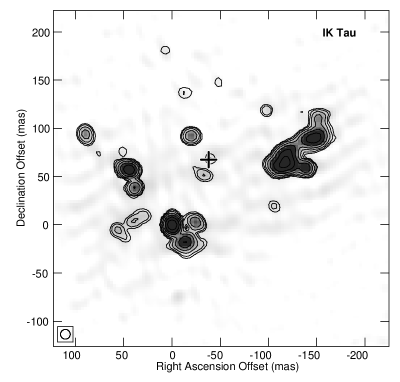
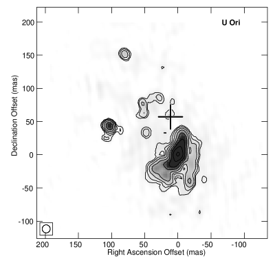
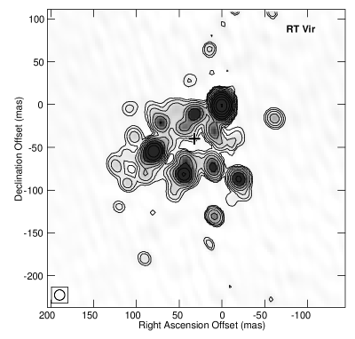
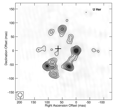
Figure 1: Integrated H₂O maser emission from four AGB stars observed by MERLIN in April 1994. The origin is at the position of the reference feature. The cross shows the estimated stellar position (Section 4.1). The restoring beam is shown in the lower left corner. The grey-scale shows all emission, the contour plots were made after blanking each channel at its $5\sigma_{\rm rms}$ level. The contour levels are at (1, 2, 4…)$\times$ the lowest contour level. This is at 0.1, 0.05, 0.3 and 0.3 Jy km s^-1 beam^-1 for IK Tau, U Ori, RT Vir and U Her respectively.

Figure 2: Top MERLIN spectrum of IK Tau 22-GHz emission. Bottom Maps of emission integrated every 12 channels. The origin is at the position of the reference feature. Each pane is labelled with the central velocity. The contour levels are (1, 2, 4…) $\times$ 0.04 Jy bm^-1. The restoring beam is shown in the first pane. The panes containing the brightest emission (at 46.4, 45.1 and 31.2 km s^-1) contain some artefacts due to dynamic range limitations.

Figure 3: Top MERLIN spectrum of U Ori 22-GHz emission. Bottom Maps of emission integrated every 10 channels. The origin is at the position of the reference feature. Each pane is labelled with the central velocity. The contour levels are (1, 2, 4…) $\times$ 0.04 Jy bm^-1. The restoring beam is shown in the first pane. The pane containing the brightest emission (at –37.4 km s^-1) contains some artefacts due to dynamic range limitations.

Figure 4: Top MERLIN spectrum of RT Vir 22-GHz emission. Bottom Maps of emission integrated every 12 channels. The origin is at the position of the reference feature. Each pane is labelled with the central velocity. The contour levels are (1, 2, 4…) $\times$ 0.07 Jy bm^-1. The restoring beam is shown in the first pane. The panes containing the brightest emission (at 23.2, 13.1 and 11.8 km s^-1) contain some artefacts due to dynamic range limitations.

Figure 5: Top MERLIN spectrum of U Her 22-GHz emission. Bottom Maps of emission integrated every 10 channels. The origin is at the position of the reference feature. Each pane is labelled with the central velocity. The contour levels are (1, 2, 4…) $\times$ 0.07 Jy bm^-1. The restoring beam is shown in the first pane. The panes containing the brightest emission (at –14.6, –15.6 and –16.7 km s^-1) contain some artefacts, mostly near the centre, due to dynamic range limitations.

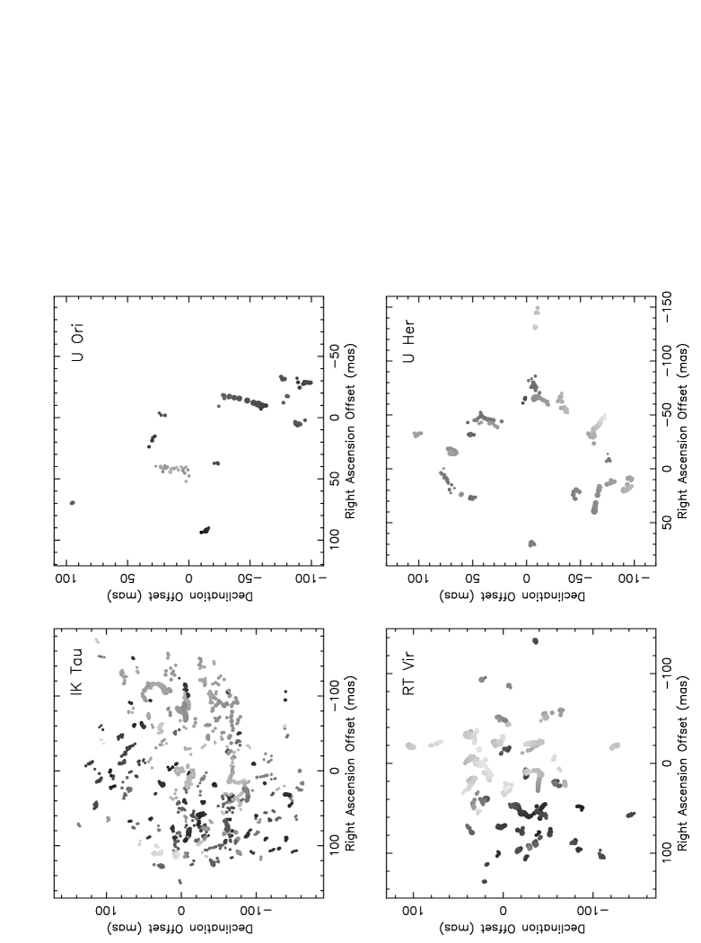
Figure 6: The positions of the H₂O maser components for each source. Each panel is labelled with the source name. The origin is at the estimated stellar position. The diameter of each spot is proportional to the logarithm of its flux density. The paler spots correspond to more blue-shifted emission and the darker spots correspond to more red-shifted emission.

3.1 MERLIN spectra and maps

Maps of the integrated 22-GHz emission from each source are shown in Figure 1. The emission comes in each case from elliptical regions $\sim$0.3 arcsec in extent, in which are embedded hot spots $\sim$20 mas in extent which contribute most of the flux. Table 3 lists for each source the total angular extent of the emission detected, at the 5$\sigma_{\rm rms}$ level $\Delta\theta_{\rm tot}$ (column(2)), together with the stellar velocity (column (3)), the minimum and maximum of Doppler velocity (columns (4) – (5)) and the range $\Delta V_{\rm LSR}$ (column (6)), the peak flux density $S_{\rm peak}$ (column (7)) and the integrated emission $S_{\rm tot}$ (column (8)). Figure 1 also shows estimated stellar positions derived in Section 4.1. It is clear that in each case the brightest emission is mostly found towards the outer parts of the H₂O envelope, with little emission from the direction of the star.

Figs. 2 to 5 show the results in more detail: a MERLIN spectrum for each source, together with maps of the emission integrated over velocity ranges of $\sim$1.2 km s^-1. Individual channel maps contain mostly well-separated, slightly resolved patches of emission. Comparison with single dish data (autocorrelations and independent monitoring e.g. ?) shows that MERLIN detected all the flux to within the errors ($\leq 10$ percent). Note however that the extreme red-shifted emission from IK Tau extends right up to (and possibly beyond) the edge of our observing band. Henceforth red- and blue-shifted are used to denote emission with $V_{\rm LSR}>V_{*}$ and $V_{\rm LSR}<V_{*}$ respectively.

Fig. 6 shows the positions of the fitted maser components in each channel, with grey-scale used to indicate velocity. In Section 5 we analyse the properties of the individual maser components. Here we concentrate on the global aspects of the maser distributions around each star. Results for each source are given in the following four Sections.

3.2 IK Tau

IK Tau has the most complex spectrum and the widest velocity range of the four sources we studied. There are two bright spectral peaks asymmetrically distributed on either side of the stellar velocity: the blue-shifted peak by 6 km s^-1 and the red-shifted peak by 12 km s^-1. The channel maps of IK Tau show that these bright emission peaks are due to multiple bright clumps spread over an elliptical region $\sim 200$ mas E-W and $\sim 100$ mas N-S. Fainter clumps of emission are found in all channels, from an almost spherical region. Moderately blue-shifted emission to the west tends to be brighter than that to the east; the opposite is true for red-shifted emission. At velocities close to $V_{*}$ a clump to the south dominates the emission. The extreme red- and blue-shifted emission features are offset towards the east.

Previous MERLIN observations by ? in 1985 detected only the bright elliptical region of emission but not the fainter spherical envelope. No individual maser features from the earlier MERLIN maps can be matched to features in the new maps. On the other hand, ? found a close correspondence between MERLIN and VLA maps made 16 months apart (?; ?). Many maser features had survived over that time period and ? were able to measure expansion of the H₂O maser envelope.

Although the overall appearance of the envelope in 1994 is of a spherically symmetric shell, nevertheless there is a clear offset between the near and far sides of the shell, with red-shifted emission mainly to the east and blue-shifted emission mainly to the west. This is particularly noticeable in Figure 6. The E-W velocity segregation can be explained if the shell has an equatorial density enhancement so that the brightest masers lie in an oblate spheroid. The plane of the equator is at an angle of inclination $i$ to the line of sight, with the eastern end of the polar axis approaching us. ? report that 3.1 $\mu$m speckle interferometry shows an approximately circular disc of warm dust 140 mas in diameter with a resolution of 40 mas. If this is the projection of the inner regions of the H₂O maser shell, with a minimum axial ratio within the uncertainty, this constrains $i\ga 45\degr$. ? fig. 2 shows model maps for an oblate spheroid at $i=45\degr$ producing an asymmetric appearance at velocities around midway between $V_{*}$ and the extreme velocities. This model does not include acceleration, which produces brighter tangential beaming. ? found that the OH mainline masers trace a biconical outflow with a wide opening angle, surrounded by OH-1612 MHz masers in the equatorial region, with $i\approx 60\degr$.

3.3 U Ori

U Ori has the narrowest velocity range of the four sources, with a single dominant spectral peak at a red-shift of 2 km s^-1 and mainly red-shifted emission. The brightest emission, at $-37.4$ km s^-1, comes from an extended region to the south west, while the remainder of the emission is to the north and east. The distribution as a whole is elongated NE-SW, at a position angle of $\sim$30°. The maser envelope is the most sparsely filled of the four we studied (Figure 6).

U Ori has been monitored at 22 GHz by ? since 1980 using the Pushchino single dish radio telescope. They observed H₂O maser flares, which they propose arise due to shocks propagating radially out from the star. Spectacular OH maser flares have also been observed (?; ? and references therein).

? mapped U Ori in 1988 using the VLA and found a similar elongated distribution at position angle $\sim$60°. The major difference between our maps and theirs is that they detected weak blue-shifted emission out to –49  km s^-1 near the centre of the distribution, close to our estimated stellar position. The position angle of the H₂O envelope observed by ? in 1988 is identical to the position angle of the OH 1612-MHz maser flare measured by Chapman & Cohen (1985) in 1983.

3.4 RT Vir

RT Vir has the greatest 22-GHz peak flux density and total flux of the four sources, with two bright spectral peaks $\sim$5 km s^-1 each side of the stellar velocity.

The emission has an angular extent $\leq 370$ mas, containing an inner ring of bright masers $\sim 150$ mas in diameter. As in IK Tau the emission contributing to the strongest spectral peaks is due to many compact maser regions spread over a large region. The total extent of the emission region is greatest near the stellar velocity and least near the extreme velocities, as expected for an expanding spherical shell, but again as in IK Tau the extreme red- and blue-shifted features are displaced from each other. Extreme blue-shifted emission from RT Vir comes from near the centre of the channel maps, but the extreme red-shifted emission is to the south east. The most extended emission consists of faint patches to the N (slightly blue-shifted) and to the south (slightly red- and blue-shifted).

The integrated emission shown in Figure 1 gives the impression of a well-filled spherically symmetrical shell, but in fact there is a systematic displacement between the near and far sides of the envelope, with most red-shifted masers to the east and blue-shifted masers to the west (Figure 6 This E-W velocity segregation can be explained if the shell has an equatorial density enhancement so that the brightest masers lie in an oblate spheroid.

Previous maps of RT Vir show a similar displacement between the near and far sides of the H₂O envelope (Imai et al. 1997, ?, ?, Bowers, Claussen & Johnston 1993). Despite this similarity, individual maser features cannot be matched.

RT Vir has been monitored at 22 GHz at Pushchino since 1985 (?; ?). It is extremely rapidly variable, with individual flares lasting less than 3 months. The MERLIN spectrum has a peak 150 Jy brighter than measured at Pushchino a month earlier.

RT Vir appears to have an equatorial density enhancement in its 22-GHz maser distribution such that the brightest emission comes from an oblate spheroid tilted in the plane of the sky so that the western side is approaching us. This structure persists much longer than the lifetime of identifiable individual maser clouds. The model maps of ? fig. 2 qualitatively illustrate the appearance of the brightest emission (as for IK Tau). The polar axis is likely to be at a projected angle similar to the direction of the red-blue velocity offset.

3.5 U Her

The emission from U Her is strongest near the stellar velocity and mainly blue-shifted. The emission comes from an elliptical ring-like region centred on our estimated stellar position, and elongated roughly north-south. The brightest emission lies to the south and west. The emission from each channel map is likewise ring-like, with no systematic change of radius with velocity. The most complete rings are seen near the stellar velocity, whereas at the extreme velocities just a single emission region is seen, offset from the stellar position by $\sim$80 mas in each case. The most red-shifted emission occurs near the inner edge of the ring towards the west. The extreme blue-shifted emission lies to the south south west. The only emission clearly outside the ring is a moderately blue-shifted spur $\sim 100$ mas to the west.

A similar ring-like distribution was observed by ? in 1988 with the VLA, when the source was an order of magnitude brighter. However there is no detailed correspondence of individual maser features between the two epochs. The extreme blue-shifted emission which formed the north-eastern part of the ring in 1988 has now faded. The radius of the ring may appear to have increased by $\sim$20 mas in the 5 years between the two set of observations, but this result is only marginally significant given the 70-mas beam of the VLA and the lack of detailed agreement at the level of individual components. ? also found a ring distribution using the VLA in 1990, but again with no detailed correspondence between individual maser features at the different epochs.

Previous MERLIN measurements by ? in 1985 detected only a single extended region of emission near the stellar velocity.

The strong differences in appearance at different epochs show that individual clouds in the envelope of U Her cannot be followed for more than $\sim$2 stellar periods. This is consistent with the shock model discussed later in Section 5.4. U Her, like U Ori, has also undergone OH maser flares  (?), which may be another result of shocks.

4 The dynamics of the circumstellar envelopes

4.1 Stellar position

Much of our further analysis requires an estimate of the stellar position. We used two methods to estimate the centre of expansion ($X$, $Y$), assumed to be the stellar position. Both methods assume that $V_{*}$ is accurately known and use least-squares minimisation routines.

The shell-fitting method of ? finds the point which is most nearly equidistant from all components in angular separation and in velocity. This assumes the maser components have a point-symmetric distribution about the centre of a spherical shell. However for non-spherical shells it is more reliable to use a method based on the quenching radius (Section 5.3). Values of ($X$, $Y$) are found which maximise the angular separation from all components with velocities within the range $V_{*}\pm(\Delta V_{\rm LSR}/n)$, where $n$ is between 4 and 8 (see Table 3).

In practice, similar results were obtained using both methods for IK Tau, RT Vir and U Her. For U Ori the shell-fitting method did not converge, but the quenching radius method gave consistent results for different values of $n$. Table 4 gives ($X$, $Y$) found by the quenching radius method. The error quoted is the difference between this position and the mean position found by all methods.

Figs. 2 to  5 (bottom) show that in all four CSEs either or both of the extreme blue- and red-shifted features are offset from the assumed stellar position by 20 – 115 mas. We did not consider the mid-point of the extreme blue- and red-shifted features as the stellar position as in every case this would be very asymmetric with respect to most of the masers. The offsets could be explained by turbulence of 1.1 – 1.6 km s^-1 (?; ?), by clumpiness, or by more systematic causes discussed in Sections 3.1 and 5.4.

Table 4: Estimated stellar positions ($X$, $Y$) with respect to the reference feature for each source.

Source	($X$, $Y$)	Error in $X$ and $Y$
	(mas)	(mas)
IK Tau	($-38$, $67$)	4
U Ori	($11$, $57$)	9
RT Vir	($32$, $-40$)	3
U Her	($65$, $7$)	5

4.2 Kinematics of the H₂O shells

Figure 7: Radius-velocity plots of the 22-GHz masers around IK Tau, U Ori, RT Vir and U Her, showing the angular separation $a$ from the assumed stellar position, as a function of $V_{\rm LSR}$. The diameter of each spot shown proportional to the logarithm of its flux density. The dashed lines show ellipses centred on $V_{*}$ which were fitted by eye to the inner and outer limits of the maser distribution. The dotted line shows an alternative inner limit for IK Tau (see Section 5.3).

Previous MERLIN observations of circumstellar H₂O masers have suggested a thick-shell model, in which the masers are distributed irregularly but the velocity field is regular and spherically symmetric, increasing steadily with radius through the H₂O maser region (?, ? and references therein). That model also describes the present observations well. In Fig. 7 we show the radius-velocity plots for the four sources. The inner and outer edges of the H₂O envelope were estimated by fitting the dashed ellipses by eye to the data. From these we obtain the inner and outer radii of the H₂O maser zone, which we denote by $r_{\rm i}$ and $r_{\rm o}$, together with the corresponding expansion velocities $v_{\rm i}$ and $v_{\rm o}$. These parameters are listed in columns (2) – (7) of Table 5. The error in the estimated stellar position (Section 4.1) is applicable to the estimates of $r_{\rm i}$ and $r_{\rm o}$ and is given in column (8) of the Table.

Two alternative inner limits are shown for IK Tau, since the limit (a) with the larger value of $r_{\rm i}$ is well defined but a few features lie within this giving a smaller value (b). The limits for U Ori and U Her are more uncertain but have been informed by the appearance of these stars at other epochs (e.g. ?, Murakawa priv. comm.) when emission appeared at different position angles and/or velocities.

In all cases the expansion velocity is less than the escape velocity at the inner edge of the H₂O maser zone, but easily exceeds the escape velocity at the outer edge of the H₂O maser envelope. This was already established by ? for IK Tau and RT Vir, and seems to be a characteristic of circumstellar H₂O envelopes in general.

The shell limits were used to derive the logarithmic velocity gradient $\epsilon=d(\ln v)/d(\ln r)$ in each circumstellar envelope. These are listed in column (9) of Table 5, along with the error $\sigma_{\epsilon}$, the linear velocity gradient $K_{\rm v}$ and its uncertainty $\sigma_{\rm K_{\rm v}}$ (in columns (10) to (12) respectively). These are average values for the H₂O maser shells as there are local variations in each CSE. Acceleration is strongest nearer the star in each case.

The values of $\epsilon$ are similar in the four stars: they range from 0.5 to 0.9, and are very similar to the values derived from MERLIN observations of supergiants (? and references therein). These are the first direct measurements of $\epsilon$ for low-mass AGB stars, since ours are the first measurements to resolve the thickness of the H₂O shells. Previous MERLIN measurements by ? made at lower angular resolution (without the Cambridge telescope) could only set upper limits on $\epsilon$ for IK Tau and RT Vir.

The total H₂O maser luminosity $\Phi$ (equivalent isotropic luminosity) is given in column (13) of Table 5 for completeness. Although the three Miras all have peaks of similar intensity (Table 3) and are at a similar distance, U Ori has only about a quarter of the luminosity of IK Tau, U Her being at an intermediate value. RT Vir is almost twice as luminous as the brightest of the Miras.

The present measurements are sufficiently detailed to allow us to investigate the variation of maser emissivity with radius in the CSEs. Figs. 7 and the spectra in Figs 2 – UHER show that more and brighter masers were detected in the inner parts of the shells. This is broadly consistent with the models of ? who predict a sharp increase in maser brightness near $r_{\rm i}$ and a gradual decline towards $r_{\rm o}$.

The 22-GHz maser shells around IK Tau and RT Vir are well-filled enough for us to estimate the photon luminosity as a function of distance from the star. We used the model of a spherically symmetric velocity field within the shell limits given in Table 5 to assign each maser component a full set of vectors to describe its position and velocity in all 3 spatial dimensions, as described in Murakawa et al. (2002, MNRAS, submitted). We then calculated the flux density in sub-shells with a cross-section in the plane of the sky of 10 mas, and used this to find the 22-GHz photon rate per unit radius $d\Phi/d{r}$. This is shown in Fig. 8. The results are robust at the 10 percent level to departures from spherical symmetry by up to a factor 2 in $\epsilon$  (?).

The results shown in Fig. 8 were compared with the model results of ?. Initially we used the mass loss rates $\dot{M}_{\rm CO}$ given in Table 1. For IK Tau $d\Phi/d{r}$ reaches a maximum value of $\sim 2\times 10^{33}$ photons s^-1 m^-1 at a radius of $6\times 10^{12}$ m. This distance is within the range predicted by the models of ? for the given $\dot{M}_{\rm CO}$. However, for RT Vir, the maximum $d\Phi/d{r}\sim 4\times 10^{33}$ photons s^-1 m^-1 occurs at a radius of $3\times 10^{12}$ m, which is $\sim 3$ times the radius predicted by ? for the given $\dot{M}_{\rm CO}$.

We return to this comparison later in Section 5.4, when we discuss the over-density of the H₂O maser clouds with respect to their surroundings.

Figure 8: The 22-GHz photon rate per unit radius for IK Tau and RT Vir, as a function of radial distance from the assumed stellar position. The bold numbers above the abscissa are estimates of the time taken for material in the stellar wind to reach that distance, see Section 5.3.

Table 5: Parameters of the H₂O maser envelopes (see Sections 4.2 and 4.3 for details).

Source	$r_{\rm i}$		$v_{\rm i}$	$r_{\rm o}$		$v_{\rm o}$	$\sigma{\rm r}$	$\epsilon$	$\sigma_{\epsilon}$	$K_{\rm v}$	$\sigma_{\rm K_{\rm v}}$	$\Phi$
	(mas)	(au)	(km s-1)	(mas)	(au)	(km s-1)	(au)			($10^{-12}$		($10^{42}$
										km s-1 m-1)		photons s-1)
(1)	(2)	(3)	(4)	(5)	(6)	(7)	(8)	(9)	(10)	(11)	(12)	(13)
IK Tau(a)	60	16.0	4.5	250	66.5	16.0	1.0	0.89	0.08	1.52	0.06	4.63
IK Tau(b)	25	6.7	5.5	250	66.5	16.0	1.0	0.46	0.09	1.17	0.04	4.63
U Ori	37	9.8	2.5	120	32.5	7.5	2.4	0.92	0.24	1.48	0.23	0.85
RT Vir	45	6.0	4.0	185	25.6	10.0	0.4	0.65	0.05	2.15	0.08	7.88
U Her	48	12.8	5.0	175	46.6	9.5	1.1	0.50	0.04	0.89	0.05	1.92

4.3 The velocity fields of the stellar winds

Fig. 9 shows plots of expansion velocity vs. radial distance for the four stars, compiled using our H₂O data together with data on other molecular species taken from the literature. All four stars have bright OH mainline masers which have been mapped (?; ?; ?; ?; ?), while IK Tau was mapped at 1612 MHz by ?. The OH 1612-MHz maser flares in U Ori were imaged by ? but as there was no clear shell structure there was no obvious way to assign a radial distance to the emission. CO data were taken from the references in Table 1. Only RT Vir is well resolved in CO  (?). The values given for the Miras are based on different models used by the various authors, but they also observed some of the same stars as ?. Comparison of the results for objects in common suggests a CO diameter of 10000 au for IK Tau, and sizes a factor of $3-5\times$ smaller than those given for U Her and U Ori. The error bars for CO data in Fig. 9 reflect this. The distances were taken as 133 pc for RT Vir and 266 pc for the other stars.

Fig. 9 show several striking features:

• There is a general increase of expansion velocity with distance from the star, with some scatter. The strongest acceleration is in the region out to 30 au in the smallest CSE, RT Vir, and 70 au in the largest, IK Tau.

• IK Tau and U Her also show evidence for gentler acceleration continuing further outwards to $\sim$500 au, and perhaps as far as the CO region at $\sim$3000 au.

• The best filled 22-GHz maser shells, around IK Tau and RT Vir, attain the greatest H₂O velocities and contain faster emission at a given radius than do the shells of U Ori and U Her.

• In U Ori, U Her and RT Vir, the OH mainline masers overlap the H₂O shells in angular separations and velocities. However the H₂O masers appear to have greater velocities than OH masers at a similar radius.

? observed acceleration of the wind from VX Sgr out to at least 100 $R_{*}$ and showed that could be explained by an increase in the dust absorption efficiency $\kappa_{\rm D}$ during the outflow. A similar kinematic pattern has been observed in other RSG e.g. S Per  (?) but hitherto it has been hard to confirm similar behaviour in the smaller CSEs of Miras. Fig. 9 and Table 5 show that acceleration occurs out to many tens of $R_{*}$ in these stars, and much further for two of the stars: IK Tau and U Her.

If dust properties are assumed to be constant ? predict that some acceleration does occur due to optical depth effects but terminal velocity is attained at $\la 10R_{*}$ and wind speed increases monotonically with $\dot{M}$ for silicate dust  (?). Monnier, Geballe & Danchi (1998, 1999) found periodic and long-term fluctuations in the shape and intensity of the 9.7$\mu$m silicate feature towards IK Tau, U Ori and U Her. This suggests changes in the dust optical constants; possible mechanisms include annealing or solid diffusion (? and references therin), which could improve the absorption efficiency at greater $r$.

Multi-epoch monitoring is continuing to investigate the effects of stellar variability on the velocity field in CSEs. ? found strong variability (“mode-switching”) in the 22-GHz line shape and velocity width towards OH 39.7+1.5, with no evidence for velocity gradients at large radial distances. However, unlike the stars in our sample, this object has cool IRAS colours and a 9.7-$\mu$m silicate feature in absorption. ? and ? also found that H₂O masers attain terminal velocity in objects with high $\dot{M}$, whereas H₂O masers in thinner-shelled CSEs do not. This is consistent with our results and suggests that stronger acceleration is favoured when starlight can more easily penetrate the CSE.

Figure 9: Expansion velocity as a function of radial distance from the four stars IK Tau, U Ori, RT Vir and U Her. The H₂O data are from Table 5. The OH data are from references given in Section 4.3. The CO values are outer limits from references given in Table 1.

5 The properties of maser clouds

Figure 10: The labelled points show the measured values of $r_{\rm i}$ as a function of $(\dot{M}_{\rm CO})^{2/3}/v_{\rm i}$. The solid line is the predicted $r_{\rm q}$ for a similar range of $\dot{M}_{\rm CO}$ at a typical $v_{\rm i}=5$ km s^-1 and $f=4\times 10^{-4}$.

5.1 Maser component sizes and temperatures

We now analyse the properties of individual water vapour maser clouds. We begin by considering the Gaussian components fitted to each channel map. In the following sections we will deal with the maser clouds themselves. Fig. 6 shows the positions of the fitted components in each channel relative to the estimated stellar position (Section 4.1) for each source. A complete list of the fitted components and their fitted parameters is available electronically via CDS.

In each source, the majority of components are resolved. Table 6 summarises component properties. The apparent size of an individual maser component $s$ (measured as described in Section 2) is the FWHM of beamed maser emission from molecules with velocities within the 0.105 km s^-1 channel width, and is smaller than the physical size of the emitting region. The greater the maser amplification factor, the smaller the beaming angle  (?), and so under comparable conditions brighter maser components appear smaller. Column (2) gives the total number $N_{\rm c}$ of 22-GHz maser components in each source and column (3) gives the fraction of components $F_{\rm c}$ for which $s>\sigma_{\rm s}$, where $\sigma_{\rm s}$ is the uncertainty in $s$. The error-weighted mean and scatter of $s$, $\overline{s}$ and $\sigma_{\overline{\rm s}}$ are given in columns (4) and (5). The scatter is intrinsic to the data, not simply due to measurement uncertainties. Note that if RT Vir is at half the distance of the other sources, $\overline{s}$ represents a similar actual size in all sources apart from U Ori, whose components appear significantly larger. ? resolved out well over half the flux from RT Vir using VLBI, but established that the brighter spots detected (mostly $>100$ Jy in the total power spectrum) had a spatial FWHM of 0.3–1.2 mas, which is consistent with our results.

The brightness temperature $T_{\rm Bc}$ of each component was calculated from its total flux density $S_{\rm c}$ and its size $s$. The minimum $T_{\rm Bc}$ measured for each source was $10^{5}$ K; the maxima are given in column (6) of Table 6. For a spherical masing region, the relationship between beamed component size and brightness temperature can be approximated by

$$s\propto\alpha\log T_{\rm Bc}.$$ (1)

? develops a more complete model giving $-1\la\alpha\la-2$ for spherical clouds, explaining how lower values correspond to more saturated maser emission if the other relevant factors are unchanged.

Figure 11: Maser component FWHM $s$ as a function of brightness temperature $T_{\rm Bc}$. The lines show error-weighted fits with slope $\alpha$ as defined in Equation 1.

Fig. 11 shows $s$ as a function of $\log T_{\rm Bc}$. We used error-weighted least-squares fits to find the slope $\alpha$, which is given in column (7) of Table 6. For IK Tau, U Her and RT Vir, the results are broadly consistent with our simplified model and imply that the masers are saturated. The formal errors in $\alpha$ are $\leq 0.2$ and values of $\alpha<-2$ may be due to the intrinsic scatter in $s$ and to deviations from our assumptions. However, for U Ori $\alpha>0$ showing more drastic revision is needed, and this is discussed in Section 5.4.

Table 6: The error-weighted statistics of maser components and their brightness temperatures, see text for details.

Source	$N_{\rm c}$	$F_{\rm c}$	$\overline{s}$	$\sigma_{\rm\overline{s}}$	Max. $T_{\rm Bc}$	$\alpha$
			(mas)	(mas)	(K)
(1)	(2)	(3)	(4)	(5)	(6)	(7)
IK Tau	1490	0.60	3	2	$5\times 10^{9}$	$-4$
U Ori	95	0.82	9	3	$2\times 10^{8}$	$+7$
RT Vir	847	0.73	6	2	$1\times 10^{11}$	$-2$
U Her	282	0.55	3	2	$1\times 10^{8}$	$-3$

5.2 Measurements of maser clouds

Fig. 6 shows the grouping of components into necklace-like strings, with similar velocities and positions. Each string is thought to be produced by a single maser cloud, with the emission in each frequency channel picking out the line of greatest amplification within the velocity range of that channel. IK Tau contains a few clouds with distinct velocity-position gradients, but most have an apparently random distribution of components with velocity. In U Ori, only two clouds have any clear structure. However, in U Her much of the blue-shifted emission is less random and in RT Vir the majority of clouds have smooth (not necessarily linear) gradients, which are also seen in Fig 7.

The measurements of each maser cloud derived from its constituent components are given in Tables available electronically from CDS. Columns (1) and (2) give the flux-weighted mean $V_{\rm LSR}$ of the cloud ($\overline{V_{\rm LSR}}$) and its total velocity width ($\Delta{V}$). Columns (3) and (4) respectively give the FWHM ($\Delta{V_{1/2}}$) of a Gaussian curve fitted to the cloud velocity profile and the uncertainty in this ($\sigma_{\rm\Delta{V}_{1/2}}$). Columns (5)–(12) give the position of the error-weighted centroid of the cloud with respect to the assumed stellar position (Section 4.1): $x$, $\sigma_{x}$, $y$ and $\sigma_{y}$ are the offsets and uncertainties in Cartesian coordinates and $a$, $\sigma_{\rm a}$, $\theta$ and $\sigma_{\theta}$ are in polar coordinates. Columns (13) and (14) respectively give the total angular extent of the cloud ($L$) and its uncertainty ($\sigma_{\rm L}$); column (15) gives the peak flux density ($I$), column (16) gives the total flux in the cloud ($S$) and column (17) gives the peak brightness temperature ($T_{\rm B}$).

Using a distance of 133 pc for RT Vir and 266 pc for the other sources, cloud angular size $L$ was converted to the cloud diameter $l$, which is likely to represent at least 85 per cent of the true unbeamed size  (?).

Figs. 12 and 13 show the distribution of $l$, $\Delta{V_{1/2}}$ and $\Delta{V}$ for each source. Individual cloud measurements of accuracy $\leq 1.5\sigma$ (mostly for clouds comprising only 3 components) are not included. Table 7 gives the properties of an average cloud around each star derived from error-weighted means of the individual cloud measurements above the threshold of $1.5\sigma$. Column (2) gives the total number $N$ of clouds in the source. Column (3) gives the number of clouds $N(l,1.5)$ with $l/\sigma_{\rm l}>1.5$, where $\sigma_{\rm l}$ is the uncertainty in $l$. The mean ($\overline{l}$) and dispersion ($\sigma_{\rm\overline{l}}$) of their diameters are given in columns (4) and (5) respectively. Columns (6) gives the number of clouds $N(\Delta{V_{1/2}}1.5)$ with $\Delta{V_{1/2}}>1.5\sigma_{\rm\Delta{V_{1/2}}}$. These were used to find the mean ($\overline{\Delta{V_{1/2}}}$) and dispersion ($\sigma_{\rm\overline{\Delta{V_{1/2}}}}$) of the velocity FWHM and of the total velocity width ($\overline{\Delta{V}}$) and the uncertainty in this ($\sigma_{\rm\overline{\Delta{V}}}$), given in columns (7) – (10).

Table 7 shows that the clouds around IK Tau have a significantly larger $\overline{l}$ and a smaller $\overline{\Delta{V}}$ than those around RT Vir. U Ori and U Her have intermediate values. The IK Tau clouds also have the smallest $\overline{\Delta{V_{1/2}}}$. Fig. 12 shows that IK Tau contains a greater number of larger clouds than the other sources. Fig. 13 shows that RT Vir and U Her have more clouds with $\Delta{V_{1/2}}>0.7$ km s^-1 than the other sources although RT Vir has almost as many with $0.4<\Delta{V_{1/2}}<0.5$ km s^-1, which is the peak range for IK Tau. The peak of the distribution of $\Delta{V}$ is at $1.6-2.0$ km s^-1 for RT Vir, three times the value for the other sources. RT Vir and IK Tau have a few clouds with $\Delta{V}\approx 3\Delta V_{\rm th}$ where $\Delta V_{\rm th}$ is the thermal line-width of H₂O at 1000 K, $\sim 1.4$ km s^-1.

Figure 12: The distribution of diameters $l$ of maser clouds in each source, for clouds with $l>1.5\sigma_{\rm l}$.

Figure 13: The distribution of the total velocity extent $\Delta{V}$ (dotted lines) and FWHM $\Delta{V_{1/2}}$ (solid lines) of maser clouds in each source for clouds with $\Delta{V_{1/2}}>1.5\sigma_{\rm\Delta{V_{1/2}}}$.

The necklace-like series of components in Fig. 6 appear to be in random directions. We searched for systematic velocity gradients within maser clouds as follows. For each cloud we attempted to fit a straight line to $u=V_{\rm LSR}-V_{*}$ as a function of position to find the gradient $u^{\prime}$, taking the goodness of fit as well as measurement errors into consideration in finding the uncertainty $\sigma_{\rm u^{\prime}}$. Columns (11), (12) and (13) of Table 7 give the number of clouds $N(u^{\prime})$ with $u^{\prime}>2\sigma_{\rm u^{\prime}}$ used to find the mean ($\overline{u^{\prime}}$) and the maximum (Max. $u^{\prime}$) of $u^{\prime}$. The minimum measurable $\overline{u^{\prime}}$ was $3\times 10^{-12}$ km s^-1 m^-1. The typical velocity gradient $u^{\prime}$ was $\sim$$20\times 10^{-12}$ km s^-1 m^-1. This is at least an order of magnitude larger than the systematic velocity gradient $K_{\rm v}$ (Table 5) within each expanding H₂O envelope. The most likely cause of this is local turbulence, which could be thermal, as $\Delta{V}$ is of the same order as $\Delta{V_{\rm th}}$, or due to shocks or differential acceleration between regions of different density or dust:gas ratio (see Section 5.3).

RT Vir has the strongest velocity gradients, with $\overline{u^{\prime}}$ more than double the $u^{\prime}$ seen for the other stars.

Table 7: The average properties of clouds around each source. See Section 5.2 for details.

Source	$N$	$N(\rm l1.5)$	$\overline{l}$	$\sigma_{\rm\overline{l}}$	$N(\Delta{V_{1/2}}1.5)$	$\overline{\Delta{V_{1/2}}}$	$\sigma_{\rm\overline{\Delta{V_{1/2}}}}$	$\overline{\Delta{V}}$	$\sigma_{\rm\overline{\Delta{V}}}$	$N(u^{\prime})$	$\overline{u^{\prime}}$	Max. $u^{\prime}$
			(au)			(km s-1)		(km s-1)			($10^{-12}$ km s-1 m-1   )
(1)	(2)	(3)	(4)	(5)	(6)	(7)	(8)	(9)	(10)	(11)	(12)	(13)
IK Tau	256	49	3.8	0.2	120	0.46	0.02	0.84	0.06	31	11	68
U Ori	14	10	3.0	0.8	7	0.68	0.12	1.07	0.24	3	17	45
RT Vir	55	26	2.2	0.2	52	0.67	0.04	1.67	0.11	18	43	190
U Her	34	24	2.6	0.3	24	0.78	0.05	1.03	0.12	9	11	23

We also decomposed $u^{\prime}$ into d$u$/d$a$ and d$u$/d$\theta$, but found no statistically significant preferred direction for the individual cloud velocity gradients.

Figure 14: The distribution of the peak brightness temperatures of maser clouds in each source.

Fig. 14 shows that the distribution of peak $T_{\rm B}$ for clouds around RT Vir reaches a maximum in a range $10\times$ hotter than for the other stars, as well as extending to values $100\times$ higher. For unsaturated masers, $\Delta{V_{1/2}}$ narrows as the maser gets brighter and then rebroadens as the maser saturates (?). Although Figs. 13 and 14 suggest a correlation between greater $\Delta{V_{1/2}}$ and $T_{\rm B}$, there is no clear relationship within the cloud measurements for each source.

5.3 Cloud densities and survival

The inner radius $r_{\rm i}$ of 22-GHz H₂O maser emission is determined by the quenching number density $n_{\rm q}$, above which the collision rate exceeds the radiative decay rate of the upper level of the maser transition. At 1200 K, for a fractional H₂O number density $f=4\times 10^{-4}n_{\rm H_{2}}$ (where $n_{\rm H_{2}}$ is the H₂ number density), $n_{\rm q}=5\times 10^{15}$  (?). ? predicted that $r_{\rm i}\propto\dot{M}^{2/3}/v_{\rm i}$. This relation is plotted in Fig. 10, using the relevant values given in Tables 1 and 5. Fig. 10 shows that the observed $r_{\rm i}$ of the four sources lie well above the inner radii inferred from $\dot{M}_{\rm CO}$. This suggests the maser clouds are denser than average for a homogenous wind, as if they were produced by localised episodes of mass loss at a higher rate.

The required mass loss rates ($\dot{M}_{\rm H_{2}O}$, uncertainty $\sigma_{\rm{\dot{M}_{\rm H2O}}}$) are derived as described in ?. These are given in column (2) and (3) of Table 8. The CO mass loss rates $\dot{M}_{\rm CO}$ are given in Table 1 and the ratio of the cloud density to the average density at a given radius is $\dot{M}_{\rm H_{2}O}/\dot{M}_{\rm CO}=f_{\rho}$, given in column (4) of Table 8. The quenching density also implies that all maser clouds at a given temperature have the same density, regardless of the mass loss rate. $\overline{l}$ is used to find the volume filling factor for the clouds $f_{\rm V}$ given in column (5) of Table 8.

We adopt $r_{\rm p}=r_{\rm i}+(r_{\rm o}-r_{\rm i})/4$ as a typical radius for the best-filled and brighest part of the shell, where the true cloud diameter is probably closest to the average measured cloud size $\overline{l}$. Following ?, we estimated the cloud density at $r_{\rm p}$ by extrapolation from $n_{\rm q}$ and used this to find the typical mass of a cloud of diameter $\overline{l}$, $M_{\rm H_{2}O}$, given in column (6).

The cloud sound crossing time $t_{\rm cs}$ is given for $\overline{l}$ in column (7). The time $t_{\rm s}$ taken for a cloud to travel from $r_{\rm i}$ to $r_{\rm o}$ is given in column (8) and used to find the apparent number of clouds formed per stellar period $N_{\rm P}$, given in column (9). Fig. 8 shows the time since the clouds left the star as a function of radius, where the time at $r_{\rm o}$ is time taken to reach $r_{\rm i}$ (assuming a constant velocity of $v_{\rm i}$ from $R_{*}$ to $r_{\rm i}$) plus $t_{\rm s}$. IK Tau appears to form more clouds per period than the other stars although the value for RT Vir is uncertain due to its irregular period.

With $t_{\rm cs}$ of about 1.5–3 yr, all of the sources have $t_{\rm cs}\sim 1/10t_{\rm s}$ making them vulnerable to turbulent disruption. Indeed, observations at other epochs (see references in Sections 3.2 – 3.5) show that individual clouds can be identified at intervals of up to 18 months but not after 2–5 yr, depending on the source. There is only indirect evidence at present as to whether this indicates that the clouds dissipate, or whether their maser emission in our direction simply decreases. The small volume of the shell occupied by clouds ($f_{\rm V}<0.01$), see Table 8, together with the long transit time for gas through the H₂O maser zone compared with the sound-crossing time for a cloud ($t_{\rm s}$ and $t_{\rm cs}$ typically 20 yr and 2 yr respectively) suggest that a change in the maser output towards us is the most likely explanation. Such a change could easily come about due to the large internal velocity gradients $u^{\prime}$ that we observe in random directions within individual maser clouds (Table 7 and Section 5.2). A direct proof of this hypothesis would be to observe clouds reappear at a later date.

The ratio $\overline{l}/r_{\rm p}$ is remarkably similar for all four stars, between 0.12 – 0.20, where the scatter is as expected from the measurement uncertainties. If the clouds originate from the star their birth radius is a fraction of the stellar radius given by $\overline{l}(R_{*}/r_{\rm p})/2R_{*}=0.08\pm 0.02R_{*}$.

Returning to Table 8, the total mass in the clouds we observe in each CSE is given in column (10) by $M_{\rm tot\;H_{2}O}=M_{\rm H_{2}O}N$ ($N$ is given in Table 7). The total mass injected at $r_{\rm i}$ during $t_{\rm s}$ is $M_{\rm tot\;inj}=t_{\rm s}\dot{M}_{\rm CO}$, given in column (11). The uncertainty in quantities derived from our measurements are $\la 50$ per cent, and comparisons with $\dot{M}_{\rm CO}$ may be less accurate.

Even allowing for such uncertainties, some trends observed in all four CSE are strongly significant.

• The maser clouds are one or two orders of magnitude denser than the surrounding gas, showing that in all these stars, mass is lost in the form of density-bounded discrete clumps.

• $M_{\rm tot\;inj}/M_{\rm tot\;H_{2}O}$ is between 1 and 5 (to within our accuracy of 50 per cent), consistent with the filling factor and overdensity of the H₂O maser clumps.

• For each star the radius of the clouds, extrapolated back to the stellar surface, is $\sim 0.1R_{*}$.

Prior to this work, the size of Mira clouds had not been measured. However, we (e.g. ?; Murakawa et al. 2002, MNRAS, submitted) have previously shown that RSG H₂O maser clouds are overdense by a similar amount, and are a similar relative size ($\sim 10$ per cent) when extrapolated back to $R_{*}$, although the absolute values of $l$, $R_{*}$, $r_{\rm i}$ and $\dot{M}$ are an order of magnitude greater for RSG. However, as befits their larger size, RSG cloud diameters are greater than the velocity resonance length and they survive for at least 9 years (Richards Yates & Cohen 1996, 1998).

These results suggest that the cloud size is not primarily determined by local physical or molecular processes in the wind such as shocks or cooling, as these would operate on the same scales around RSG as around AGB stars. It could be that clumps somehow grow between the star and $r_{\rm i}$, so the larger $\dot{M}$ and $r_{\rm q}$ of RSG means the clouds reach a larger mass. Alternatively, the cloud size could be directly determined at the stellar surface, related to convection cells (possibly producing local chemical enrichment), pulsation irregularities producing ejections, or cooling above starspots  (?).

Table 8: The estimates of mass loss rate from H₂O maser measurements compared with those using CO observations, the maser cloud filling factor and other properties. See Section 5.3 for details.

Source	$\dot{M}_{\rm H_{2}O}$	$\sigma_{\rm{\dot{M}_{\rm H2O}}}$	$f_{\rho}$	$f_{\rm V}$	$M_{\rm H_{2}O}$	$t_{\rm cs}$	$t_{\rm s}$	$N_{\rm P}$	$M_{\rm tot\;H_{2}O}$	$M_{\rm tot\;inj}$
	($10^{-6}$M⊙ yr-1)				($10^{-9}$ M⊙)	(yr)	(yr)		($10^{-6}$M⊙)	($10^{-6}$M⊙)
(1)	(2)	(3)	(4)	(5)	(6)	(7)	(8)	(9)	(10)	(11)
IK Tau(a)	$117$	$19$	50	0.0043	257	3.0	26	11	66	68
IK Tau(b)	$25$	$10$	10	0.0043	62	3.0	29	10	16	75
U Ori	$25$	$12$	110	0.0014	141	2.4	24	1	2	6
RT Vir	$15$	$2$	115	0.0044	44	1.7	14	2	2	2
U Her	$83$	$14$	240	0.0008	104	2.0	23	1	4	8

5.4 Maser amplification

Maser amplification occurs over a velocity resonance length $\delta l$ where $V_{\rm LSR}$ changes by $\Delta V_{\rm th}$. Inspection of the individual channel maps (Figs. 2–4) shows that there is only occasional blending, and the low filling factors imply there is $<1$ per cent chance of extra amplification due to one cloud overlapping another along the line of sight unless their distribution is very non-random. The actual clouds could be any shape, but for simplicity we assume they are spherical (however see Section 5.4). Using the method applied to the RSG S Per by ? and the shell parameters in Table 5, we estimate $\delta l$ for each source at $r_{\rm p}$ in the limiting cases of a cloud along the line of sight to the star (radial beaming) and in the plane of the sky with the star (tangential beaming). We find for IK Tau $6\ga\delta l\ga 5$, for U Ori $\delta l\approx 6$, for U Her $10\ga\delta l\ga 5$ and for RT Vir $4\ga\delta l\ga 3$ au. The radially-beamed $\delta l$ exceeds the tangentially-beamed value by a larger amount for smaller values of the logarithmic velocity gradient $\epsilon$. In all cases $\delta l>\overline{l}$ (Table 7), so the velocity coherence depth is not limiting the amplification path, unless there is some systematic asymmetry in the distribution of cloud shapes.

If the only force on clouds is due to radiation pressure on dust, their diameter in the tangential and radial directions will increase proportional to $r/r_{\rm i}$ and $(r/r_{\rm i})^{\epsilon}$ respectively. If the clouds are on average initially spherical, they will retain their shape where $\epsilon$ is not much less than 1. However, the clouds near $r_{\rm i}$ could be flattened by shocks due to the stellar pulsations. This favours tangential 22-GHz emission, perpendicular to the direction of the shock, not only due to the longer path length for maser amplifcation, but also because the pump IR photons escape along the short axis (?). In this geometry, the beaming angle is independent of $T_{\rm B}$ and the observed component angular size is equivalent to the projected width of the flattened cloud (?).

Thus, shock compression would explain the large scale of emission inferred from the visibilities in the brightest channel of U Ori (Section 3.3) and its large values of $\alpha$ and $\overline{s}$ in Table 6. The ring-like appearance of the masers around U Her is also consistent with shocked clouds. For unsaturated masers, $T_{\rm B}$ is roughly exponentially proportional to a linear function of the path length. The brightest masers around U Her have $T_{\rm B}\approx 10^{8}$ K. If this arises from clouds with an axial ratio of 2:1 viewed along the long axis, clouds viewed along the short axis will have $T_{\rm B}\approx 10^{4}$ K, so clouds lying close to the line of sight to the star are well below the detection threshold. The average cloud diameter $\overline{l}$ was calculated on the basis of spherical clouds. If we only detect flattened clouds, $l$ becomes the long axis, leading to an overestimate of $\overline{l}$. However, if the clouds around the front and back caps are present but not detected, then $N$ and $N_{\rm P}$ are underestimated but the accuracy of other quantities given in Table 8 is not greatly affected.

The 22-GHz photon luminosity rate from the whole of each shell, $\Phi$, is shown in column (13) of Table 5. For the Miras, the average $d\Phi/dr$ is $(0.3-0.6)\times 10^{30}$ photons s^-1 m^-1 but for RT Vir it is $3\times 10^{30}$ photons s^-1 m^-1, i.e. $\la 10\times$ higher. The individual masers around RT Vir also reach the highest $T_{\rm B}$, although this object has the lowest $\dot{M}$, the smallest shell and the smallest clouds. It also has the smallest, most irregular, stellar pulsations. It shows the largest velocity gradients ($u^{\prime}$ and $K_{\rm v}$) and it is the only source with $\overline{\Delta{V}}>\Delta{V_{\rm th}}$ (Table 7). The masers are very rapidly variable, suggesting highly efficient but unsaturated amplification. Small clouds with a steep velocity gradient could allow the clouds to remain optically thin at the IR pump photon frequencies (?, ?) and achieve very efficient 22-GHz maser pumping. This is analogous to the suggested enhanced masing from shock-compressed clouds in U Her and U Ori. Shock compression alone is a less likely explanation in the case of RT Vir as its bright masers extend well beyond $r_{\rm i}$ and its optical period and amplitude are poorly defined and small (Table 1), suggesting the stellar pulsations are either weak or very complex.

Another possiblity is that the wind from RT Vir is richer in H₂O. The latter could be due to a higher O:C ratio, suggesting RT Vir had a higher progenitor mass and/or is more highly evolved than the Miras (since all 4 stars are so nearby that the overall Galactic metallicity gradient has little effect although local fluctuations are possible). ? showed that, for unsaturated masers, $d\Phi/dr$ increases by up to an order of magnitude if the fractional abundance of H₂O, $f$=[H₂O]/[H₂], increases by a factor of 2. $n_{\rm q}$ is weakly dependent on $f$, so the clouds around RT Vir could be even denser by a factor of a few tenths. This could increase the acceleration of the gas, but only slightly, as the momentum coupling with the dust is already good for most of the density range in the H₂O maser clouds (?).

For IK Tau and RT Vir we were able to estimate the photon luminosity as a function of distance from the star (Section 4.2). This is shown in Fig. 8. Comparing our results with the models by ? we found that the emissivity was 100-1000 times greater than predicted for the mass-loss rates based on CO, $\dot{M}_{\rm CO}$. This difference can be explained in terms of the clumping of the mass-loss into the discrete clouds we observe. The collision rate (and hence the maser pump rate) is proportional to $\rho^{2}$, where $\rho$ is the local density. Thus, the postulated over-density of the maser clouds should increase the maser luminosity at the same radius.

From Table 8, the IK Tau maser clouds are over-dense by a factor $f_{\rho}\sim 10-50$, suggesting that the emission at an equivalent distance from the star should be $\geq 100$ times brighter than the value deduced from $\dot{M}_{\rm CO}$. This is consistent with the models of ? for a fractional H₂O density of $f\leq 2\times 10^{-4}$. However, other factors may be involved as the profile of $d\Phi/d{r}$ as a function of $r$ is very irregular, which implies changes in the rate or composition of mass loss from IK Tau as well as possible axisymmetry of the CSE.

For RT Vir, the clouds are over-dense by a factor of $f_{\rho}\sim 115$. This suggests that $d\Phi/d{r}$ should exceed the value deduced from $\dot{M}_{\rm CO}$ by a factor of roughly $115^{2}/(3^{2})^{2}$, i.e. 1–200. In fact, RT Vir is brighter than the models of ? by 3 orders of magnitude, even for the highest fractional H₂O density considered, $f=6\times 10^{-4}$.

6 Summary and conclusions

MERLIN 22-GHz observations of the 4 low-mass AGB stars IK Tau, U Ori, RT Vir and U Her show that the H₂O masers surrounding each star are found in thick expanding shells of a few hundred mas in diameter. The inner and outer limits to the maser distributions were derived, under the assumption of spherically symmetric expansion. The inner radii $r_{\rm i}$ are at 6–16 au, with outer limits $\sim$4 times greater. The maser velocity increases two- or three-fold over this distance, giving a logarithmic velocity gradient $\epsilon$ in the range $0.5\leq\epsilon\leq 1$.

For the first time, the individual 22-GHz masers in each CSE have been resolved. The unbeamed H₂O vapour cloud diameter $l$ is about 2–4 au at a distance of 10–25 au from the star. If the clouds are formed close to the stellar surface, assuming linear expansion, this corresponds to an original cloud radius of $\sim 0.1R_{*}$. We find that $l$ is less than the velocity resonance length for spherical clouds. The average cloud velocity span is 0.8–1.7 km s^-1, with a FWHM between 0.5–0.8 km s^-1.

The water vapour cloud density at $r_{\rm i}$ is one or two orders of magnitude greater than the mean density derived from the mass loss rates inferred from CO and other observations. The volume filling factor of the shells is $<0.5$ per cent. In addition, we find that the clouds are vulnerable to disruption by shocks during the passage through the shell, as the sound crossing time ($t_{\rm cs}$) of the clouds and the time the cloud takes to travel through the maser shell ($t_{\rm s}$) are related by $t_{\rm cs}\sim(1/10)t_{\rm s}$. These facts suggest that the masers are density bounded. We find that the maser survival times and sizes of clouds around these AGB stars are $\sim 10$ times smaller than those around RSG, approximately the same ratio as the stellar masses and sizes. This implies that it is the properties of the central star that determine maser cloud sizes, rather than behaviour intrinsic to the wind.

U Ori and U Her have poorly-filled H₂O maser shells and both have shown OH maser flares. Some individual 22-GHz maser components in U Ori have a large beamed size which does not decrease with increasing $T_{\rm B}$, indicative of masing from a slab rather than a sphere. In U Her, the masers form a hollow ring. The appearance of the 22-GHz masers in both of these sources suggests that they emanate from shock-compressed shells, producing strong tangential amplification; such shocks could be the cause of the OH flares.

IK Tau and RT Vir have well-filled H₂O maser shells. Observations of both of these sources made $\la$ 10 years apart show a persistent E-W offset between moderately red- and blue-shifted emission, although individual masers do not survive more than $\sim 1.5$ yr. This can be explained by an equatorial density enhancement in a spherical shell, so that the brightest masers lie in an oblate spheroid and the equatorial plane is at an angle $i$ to the line of sight, such that $\pi/2>i>\pi/4$. At any one epoch, the shells of U Her and U Ori appear asymmetric, but after comparing our maps with those published at different epochs (see Section 4 for references), we cannot distinguish any systematic deviations from poorly-filled spherical shells.

We are obtaining multi-epoch maps of H₂O and OH masers using MERLIN and the EVN to provide similar resolution for all species. This will allow us to study the evolution of individual maser clouds. We will measure their proper motions and distinguish between acceleration and any latitude dependence of expansion velocity e.g. a bipolar outflow. We will thus examine the stability of the velocity field in the CSE as a whole and maser amplification within individual clouds. We will measure changes in maser size and brightness with time and so constrain the degree of maser saturation and the local overdensity of maser clouds as a function of radius. We will develop a fuller model of the velocity fields to compare with predictions based on dust properties and distribution.

7 Acknowledgements

MERLIN is the Multi Element Radio Linked Interfermometer Network, a national facility operated by the University of Manchester at Jodrell Bank Observatory on behalf of PPARC. We thank the MERLIN staff for performing the observations. In this research we have used, and acknowledge with thanks, data from the AAVSO database submitted to the AAVSO by variable star observers worldwide. DRG gratefully acknowledges a research grant from CONACYT, the Mexican Research Council, and an EC Marie Curie studentship at the IoA Cambridge.

References

- [Bieging et al.¡2000¿] Bieging J. H., Shaked S., Gensheimer P. D., 2000, ApJ, 543, 897
- [Blöcker¡1995¿] Blöcker T., 1995, A&A, 297, 727
- [Bowen¡1988¿] Bowen G. H., 1988, ApJ, 329, 299
- [Bowers & Johnston¡1988¿] Bowers P. F., Johnston K. J., 1988, ApJ, 330, 339
- [Bowers & Johnston¡1994¿] Bowers P. F., Johnston K. J., 1994, ApJS, 92, 189
- [Bowers et al.¡1993¿] Bowers P. F., Claussen M. J., Johnston K. J., 1993, AJ, 105, 284
- [Bowers¡1991¿] Bowers P. F., 1991, ApJS, 76, 1099
- [Bujarrabal et al.¡1989¿] Bujarrabal V., Gómez-González J., Planesas P., 1989, A&A, 219, 256
- [Chapman & Cohen¡1985¿] Chapman J. M., Cohen R. J., 1985, MNRAS, 212, 375
- [Chapman & Cohen¡1986¿] Chapman J. M., Cohen R. J., 1986, MNRAS, 220, 513
- [Chapman et al.¡1991¿] Chapman J. S., Cohen R. J., Saikia D. J., 1991, MNRAS, 249, 227
- [Chapman et al.¡1994¿] Chapman J. S., Sivagnanam P., Cohen R. J., LeSqueren A. M., 1994, MNRAS, 268, 475
- [Chapman¡1985¿] Chapman J. M., 1985, PhD thesis, University of Manchester
- [Cohen¡1989¿] Cohen R. J., 1989, Reports on Progress in Physics, 52, 881
- [Colomer et al.¡2000¿] Colomer F., Reid M. J., Menten K. M., Bujarrabal V., 2000, A&A, 355, 979
- [Condon et al.¡1998¿] Condon J. J., Cotton W. D., Greisen E. W., Yin Q. F., Perley R. A., Taylor G. B., Broderick J. J., 1998, AJ, 115, 1693
- [Condon¡1997¿] Condon J. J., 1997, PASP, 109, 166
- [Cooke & Elitzur¡1985¿] Cooke B., Elitzur M., 1985, ApJ, 295, 175
- [Elitzur & Ivezić¡2001¿] Elitzur M., Ivezić Ž., 2001, MNRAS, 327, 403
- [Elitzur et al.¡1992¿] Elitzur M., Hollenbach D. J., McKee C. F., 1992, ApJ, 394, 221
- [Elitzur¡1992¿] Elitzur M., 1992, Astronomical Masers. Kluwer
- [Engels et al.¡1988¿] Engels D., Schmid-Burgk J., Walmsley C. M., 1988, A&A, 191, 283
- [Engels et al.¡1997¿] Engels D., Winnberg A., Walmsley C. M., Brand J., 1997, A&A, 322, 291
- [Etoka & Le Squeren¡1997¿] Etoka S., Le Squeren A. M., 1997, A&A, 321, 877
- [Etoka et al.¡2001¿] Etoka S., Blaskiewicz L., Szymczak M., Le Squeren A. M., 2001, A&A, 378, 522
- [Frank¡1995¿] Frank A., 1995, AJ, 110, 2457
- [Gail & Sedlmayr¡1994¿] Gail H. P., Sedlmayr E., 1994, in Hartquist T. W., A W. D., eds, The Molecular Astrophysics of Stars and Galaxies. Oxford University Press, p. 285
- [Gail & Sedlmayr¡1998¿] Gail H. P., Sedlmayr E., 1998, in Sarre P., ed, Chemistry and Physics of Molecules and Grains in Space. Faraday Discussion 109. RSC, London, p. 303
- [Gail & Sedlmayr¡1999¿] Gail H. P., Sedlmayr E., 1999, A&A, 347, 594
- [Groenewegen et al.¡1999¿] Groenewegen M. A. T., Baas F., Blommaert J. A. D. L., Stehle R., Josselin E., Tilanus R. P. J., 1999, A&AS, 140, 197
- [Hale et al.¡1997¿] Hale D. D. S. et al., 1997, ApJ, 490, 407
- [Hipparcos Catalogue, The¡1997¿] Hipparcos Catalogue, The, 1997. ESA SP-1200, CDS-VizieR
- [Imai et al.¡1997¿] Imai H. et al., 1997, A&A, 317, L67
- [Jura¡1993¿] Jura M., 1993, in Cassinelli J. P., Churchwell E. B., eds, Massive Stars: Their Lives in the Interstellar Medium. p. 307
- [Kerschbaum & Hron¡1992¿] Kerschbaum F., Hron J., 1992, A&A, 263, 97
- [Kerschbaum & Olofsson¡1999¿] Kerschbaum F., Olofsson H., 1999, A&AS, 138, 299
- [Kholopov et al.¡1998¿] Kholopov P. N. et al., 1998, in Combined General Catalogue of Variable Stars, 4.1 Ed (II/214A). (1998)
- [Kirrane¡1987¿] Kirrane T.-M., 1987, PhD thesis, University of Manchester
- [Knapp & Morris¡1985¿] Knapp G. R., Morris M., 1985, ApJ, 292, 640
- [Knapp et al.¡1998¿] Knapp G. R., Young K., Lee E., Jorissen A., 1998, ApJS, 117, 209
- [Lane et al.¡1987¿] Lane A. P., Johnston K. J., Bowers P. F., Spencer J. H., Diamond P. J., 1987, ApJ, 323, 756
- [Lekht et al.¡1999¿] Lekht E. E., Mendoza-Torres J. E., Pashchenko M. I., Berulis I. I., 1999, A&A, 343, 241
- [Mendoza-Torres et al.¡1997¿] Mendoza-Torres J. E., Lekht E. E., Pashchenko M. I., Berulis I. I., 1997, A&AS, 126, 257
- [Monet et al.¡1998¿] Monet D. et al., 1998. USNO-A V2.0, A Catalog of Astrometric Standards, CDS-VizieR
- [Monnier et al.¡1998¿] Monnier J. D., Geballe T. R., Danchi W. C., 1998, ApJ, 502, 833
- [Monnier et al.¡1999¿] Monnier J. D., Geballe T. R., Danchi W. C., 1999, ApJ, 521, 261
- [Netzer & Elitzur¡1993¿] Netzer N., Elitzur M., 1993, ApJ, 410, 701
- [Neufeld & Melnick¡1991¿] Neufeld D. A., Melnick G. J., 1991, ApJ, 368, 215
- [Nyman et al.¡1986¿] Nyman L.-A., Johansson L. E. B., Booth R. S., 1986, A&A, 160, 352
- [Olnon et al.¡1986¿] Olnon F. M. et al., 1986, A&AS, 65, 607
- [Olofsson et al.¡1998¿] Olofsson H., Lindqvist M., Nyman L.-A., Winnberg A., 1998, A&A, 329, 1059
- [Pataki & Kolena¡1974¿] Pataki L., Kolena J., 1974, Bull. Am. astr. Soc., 6, 340
- [Richards et al.¡1996¿] Richards A. M. S., Yates J. A., Cohen R. J., 1996, MNRAS, 282, 665
- [Richards et al.¡1998¿] Richards A. M. S., Yates J. A., Cohen R. J., 1998, MNRAS, 299, 319
- [Richards et al.¡1999¿] Richards A. M. S., Yates J. A., Cohen R. J., 1999, MNRAS, 306, 954
- [Richards et al.¡2000¿] Richards A. M. S., Cohen R. J., Murakawa K., Yates J. A., van Langevelde H. J., Gray M. D., Masheder M. R. W., Szymczak M. D., 2000, in J.E. Conway A.G. Polatidis R. B., Pihlström Y., eds, Prodeecings of the 5th EVN Symp. Onsala Space Observatory, Gothenburg, p. 185
- [Richards¡1997¿] Richards A. M. S., 1997, PhD thesis, University of Manchester
- [Rudnitskij et al.¡2000¿] Rudnitskij G. M., Mendoza-Torres J. E., Pashchenko M. I., Berulis I. I., 2000, A&AS, 146, 385
- [Stanek et al.¡1995¿] Stanek K. Z., Knapp G. R., Young K., Phillips T. G., 1995, ApJS, 100, 169
- [Szymczak & Engels¡1995¿] Szymczak M., Engels D., 1995, A&A, 296, 727
- [van der Veen & Habing¡1988¿] van der Veen W. E. C. J., Habing H. J., 1988, A&A, 184, 125
- [van Langevelde et al.¡2000¿] van Langevelde H. J., Vlemmings W., Diamond P. J., Baudry A., Beasley A. J., 2000, A&A, 357, 945
- [Vassiliadis & Wood¡1993¿] Vassiliadis E., Wood P. R., 1993, ApJ, 413, 641
- [Vassiliadis & Wood¡1994¿] Vassiliadis E., Wood P. R., 1994, ApJS, 92, 125
- [Whitelock et al.¡1994¿] Whitelock P. A., Menzies J. W., Feast M. W., Marang F., Carter B. S., Roberts G., Catchpole R. M., Chapman J. M., 1994, MNRAS, 267, 711
- [Whittet¡1992¿] Whittet D. C. B., 1992, Dust in the Galactic Environment. IOP
- [Yates & Cohen¡1994¿] Yates J. A., Cohen R. J., 1994, MNRAS, 270, 958
- [Yates et al.¡1997¿] Yates J. A., Field D., Gray M. D., 1997, MNRAS, 285, 383
- [Yates¡1993¿] Yates J. A., 1993, PhD thesis, University of Manchester
- [Young et al.¡1993¿] Young K., Phillips T. G., Knapp G. R., 1993, ApJ, 409, 725
- [Young¡1995¿] Young K., 1995, ApJ, 445, 872