The Hubble Diagram of Type Ia Supernovae as a Function of Host Galaxy Morphology

Abstract

We present new results on the Hubble diagram of distant type Ia supernovae (SNe Ia) segregated according to the type of host galaxy. This makes it possible to check earlier evidence for a cosmological constant by explicitly comparing SNe residing in galaxies likely to contain negligible dust with the larger sample. The cosmological parameters derived from these SNe Ia hosted by presumed dust-free early-type galaxies supports earlier claims for a cosmological constant, which we demonstrate at $\simeq 5\sigma$ significance, and the internal extinction implied is small even for late-type systems ($A_{B}<0.2$). Thus, our data demonstrate that host galaxy extinction is unlikely to systematically dim distant SNe Ia in a manner that would produce a spurious cosmological constant. We classify the host galaxies of 39 distant SNe discovered by the Supernova Cosmology Project (SCP) using the combination of Hubble Space Telescope STIS imaging, Keck-II ESI spectroscopy and ground-based broad-band photometry. The distant data are analysed in comparison with a low-redshift sample of 25 SNe Ia re-calibrated according to the precepts of the SCP. The scatter observed in the SNe Ia Hubble diagrams correlates closely with host galaxy morphology. We find, as expected, this scatter is smallest for SNe Ia occurring in early-type hosts and largest for those occurring in late-type galaxies. Moreover, SNe residing in early-type hosts appear only $\simeq 0.14\pm 0.09$ mag brighter in their light-curve-width-corrected luminosity than those in late-type hosts, implying only a modest amount of dust extinction even in the late-type systems. As in previous studies, these results are broadly independent of whether corrections based upon SN light-curve shapes are performed. We also use our high-redshift dataset to search for morphological dependencies in the SNe light-curves, as are sometimes seen in low-redshift samples. No significant trends are found, possibly because the range of light-curve widths is too limited.

1 Introduction

Type Ia supernovae (SNe Ia) have emerged as important probes of the cosmological world-model. Although their physical properties are still not fully understood, by exploiting an empirical relationship between the peak intrinsic luminosity and the light-curve decay time (Phillips, 1993; Riess et al., 1995, 1996; Hamuy et al., 1996b; Perlmutter et al., 1997), the dispersion in their photometric properties can be reduced to $\simeq 0.17\,\mathrm{mag}$, making them valuable ‘calibrated candles’ over a wide range in redshift (e.g. Hamuy et al., 1996c).

Although numerous alternative probes of the cosmological parameters are now available (Jaffe et al., 2001; Peacock et al., 2001; de Bernardis et al., 2002; Efstathiou et al., 2002), in principle the SN Ia Hubble diagram provides the only direct measure of the cosmic expansion history free from any model assumptions. The systematic detection (Perlmutter, 1997) and photometric calibration of high redshift SNe Ia has led to two independent SN Ia Hubble diagrams, published by the Supernova Cosmology Project (hereafter SCP; Perlmutter et al., 1997, 1998, 1999) and the High-Redshift Supernova Search Team (hereafter HZT; Schmidt et al., 1998; Riess et al., 1998). Data from both teams convincingly reject the deceleration expected from an Einstein–de Sitter (EdS) Universe, and provide new evidence for a cosmic acceleration in a low mass-density Universe consistent with a non-zero vacuum energy density. Evidence for spatial flatness from microwave background experiments (de Bernardis et al., 2000; Balbi et al., 2000; Jaffe et al., 2001) further strengthens these conclusions (see e.g. Bahcall et al., 1999).

Such important results demand excellent supporting evidence. In particular, it is necessary to examine the homogeneity, environmental trends and evolutionary behaviour of SNe Ia. It must be remembered that it is not yet clear whether these events are produced by a single mechanism in a unique physical environment. Systematic differences in the peak magnitudes between high and low-redshift SNe, arising either from evolutionary effects in the SNe progenitors or via subtle differences in the environments of the low and high-redshift galaxies in which SNe are produced, could mimic the cosmic acceleration without necessarily destroying the small dispersion seen in existing Hubble diagrams.

Differences between low and high-redshift SNe Ia might arise via differing progenitor compositions (Umeda et al., 1999; Höflich et al., 2000; Domínguez et al., 2001), different progenitor ages (Ruiz-Lapuente, Canal, & Burkert, 1997), greater amounts of dust in high-redshift environments, either in the host galaxy (Hatano, Branch, & Deaton, 1998; Totani & Kobayashi, 1999; Rowan-Robinson, 2002) or in the intergalactic medium (Aguirre, 1999; Aguirre & Haiman, 2000), or a dependence of the SNe properties on host galaxy environments. Tests for analysing SNe by the type of their host galaxy were discussed by Perlmutter et al. (1997, hereafter P97), and continued by Perlmutter et al. (1999, hereafter P99). This initial classification based on host galaxy spectra revealed no changes in the properties of SNe located in E/S0 and spiral hosts, though only 17 hosts could be classified and little morphological information was available.

Continuing these studies, via an examination of the dependence of SN properties on host galaxy morphology via Hubble Space Telescope (HST) imaging and Keck spectroscopy, forms the basis of the present analysis. Although SNe Ia can occur in all types of galaxies, disc and spheroidal stellar populations will represent different star-formation histories, metallicities and dust content. Thus we might expect that SNe Ia progenitor composition and peak magnitudes or light-curve properties could be affected accordingly.

Much of the previous work examining the environments of SNe Ia has been conducted using low-redshift samples, with only limited work at high-redshift. However, in these low-redshift studies, two interesting trends have already been claimed, both of which are relevant for this present paper. The first correlates the form of the SN light-curve with the host-galaxy properties. Filippenko & Sargent (1989) originally found that the initial post-maximum decline rate in the light-curve in the $B$-band may have a smaller dispersion among SNe located in elliptical galaxies. Using SNe Ia discovered via the Calan-Tololo (C-T) SN survey (Hamuy et al., 1996a), Hamuy et al. (1996b) also note that the post-maximum decline rate correlates with morphology, in the sense that SNe with more rapidly declining light-curves (i.e. intrinsically dimmer SNe) occur in earlier-type galaxies. In an independent study of the CfA SN sample, Riess et al. (1999) find a similar result. The various low-redshift SN samples were later combined in a single analysis by Hamuy et al. (2000). They confirm the findings of the C-T and CfA studies, and also note that intrinsically brighter SNe tend to occur in bluer stellar environments (see also Branch, Romanishin, & Baron, 1996), and suggest that the intrinsically brightest SNe occur in the least luminous galaxies. These effects were further investigated by Howell (2001), who find that in the local Universe over-luminous SNe arise in spiral and other late-type systems, whilst spectroscopically under-luminous SNe tend to occur in older (E/S0) systems.

The second suggested correlation relates the photometric properties of a SN to its physical location in the host galaxy. Wang, Hoeflich, & Wheeler (1997), using SNe from the C-T survey as well as 11 other well-studied nearby SNe, found that SNe properties apparently vary with projected distance from the centre of the host galaxy. They find that SNe located more than 7.5 kpc from the centre show around 3 – 4 times less scatter in maximum brightness than those within that projected radius, with E/S0 galaxies dominating the sample at high separations. Monte-Carlo simulations exploring the effects of dust on radial distributions of SNe Ia (Hatano, Branch, & Deaton, 1998) similarly predict that SNe at large projected radial distances should be practically unextinguished, whilst those at small projected distances could suffer significant amounts of extinction. The conclusion is that SNe at higher projected distance are a more homogeneous group and should be better distance indicators.

In a combined C-T/CfA sample, Riess et al. (1999) find that SNe Ia with faster decline rates (i.e. intrinsically fainter SNe) occur at larger projected distances from the host galaxy centre. The Hamuy et al. (2000) sample has also been used by Ivanov, Hamuy, & Pinto (2000) for a similar purpose, though importantly using de-projected galactocentric distances rather than simple projected distances. This refinement suggests that the earlier Riess et al. (1999) trend may partly be due to the mix of E/S0 and spiral galaxies, with (intrinsically fainter) SNe hosted by E/S0 galaxies being discovered at larger galactic distances when compared to SNe located in spiral galaxies. No significant trend is seen in SN parameters with galactocentric distance for the E/S0 subset of the SN host population. As elliptical galaxies show radial gradients in their stellar properties arising mostly from trends in metallicity rather than age, it is concluded that the intrinsic diversity in SN parameters more likely arises from stellar population differences rather than progenitor metallicity alone (Ivanov et al., 2000). The only relevant study for high-redshift samples is that of Howell, Wang, & Wheeler (2000), based on SCP IAU circulars and finding charts. These authors examine the radial distribution of the SCP SNe from their host galaxies, and find that they are distributed similarly to those from low-redshift CCD-based samples.

The major difficulty in interpreting these trends lies in disentangling all of the numerous variables (morphology, radial position, luminosity, metallicity, dust content and star-formation history) which define the stellar populations of galaxies. Though no complete physical picture has yet emerged as to how the underlying stellar population might influence SN properties in the manner proposed, one possible hypothesis is as follows (Umeda et al., 1999).

SNe Ia most likely originate via the thermonuclear explosion of a carbon-oxygen (CO) white dwarf (WD) in a binary system, with the light-curve powered by the decay of ⁵⁶Ni. Hence, WDs with a larger ¹²C mass fraction will generate more ⁵⁶Ni and consequently brighter SNe. As the oldest progenitors are likely to have the lowest mass companions, less mass can be transferred to the primary WD, and the resultant reduced final ¹²C abundance leads to a smaller ⁵⁶Ni mass, and therefore fainter events. In this simple picture, one expects firstly to see more variation in SN properties in disc-based systems (where the age of the stellar population is more diverse) than in spheroidal galaxies, and secondly to see fewer over-luminous events in (presumably) older E/S0 systems.

So far as the implications for the use of SNe Ia as cosmological probes are concerned, we are, of course, interested in possible trends in the above correlations with redshift. Our aim is to include SNe located at high redshift which are used in existing Hubble diagrams to constrain the cosmological parameters. Environmental effects on the determination of the cosmological parameters can then be more easily explored. An outline of the paper follows. In $\S$2 we discuss the low and high-redshift SN samples used in our analysis and describe the method utilised to align them on to the same calibration system. $\S$3 introduces our new dataset, based primarily on HST imaging and Keck spectroscopy, used to investigate the properties of the host galaxies of the high-redshift sample. We discuss the classification system for the hosts in $\S$4, and present our analyses in $\S$5 and discussion in $\S$6. We present our conclusions in $\S$7.

2 The Supernova Samples

In order for us to explore the cosmological consequences of possible correlations between the SN properties and those of the host galaxies, we need samples of SNe Ia spanning the full range in redshift in the Hubble diagram analyses.

For the distant SNe Ia, we perform the analysis on the published sample of 42 SNe discovered by the Supernova Cosmology Project (SCP; see P99). All SNe were discovered by the SCP and details of the various procedures and analysis techniques, as well as spectroscopic verification, can be found in P97 and P99.

The bulk of our sample overlaps with the P99 set but this overlap is not complete by virtue of the random manner in which HST snapshot observations are selected. For example, only 30 of the 42 have HST imaging providing host galaxy morphologies. P99 further restrict this sample of 42 SNe to one of 38 high-redshift objects in the primary cosmological fit (‘fit-C’ in P99) by excluding those SNe considered ‘likely reddened’ or which are ‘outliers’ in terms of their stretch of the light-curve time-scale values. Where appropriate in this current analysis we also note the effect of excluding these 4 objects.

At lower redshifts, we use the Hamuy et al. (1996a) SNe sample and add selected SNe from the Riess et al. (1999) local sample. Our principal criteria in selecting SNe from these local samples remains as in P99, namely (i) each SN must have been observed prior to 5 days after maximum light so as to reduce any extrapolations necessary to fit peak luminosities, and (ii) that each SN has $cz>3000\,\mathrm{km\,s^{-1}}$ to control the impact of peculiar velocities. These requirements mean that 18 of the 29 C-T SNe (see P99 for details) and 12 of the 22 Riess et al. (1999) CfA SNe are included in our low-redshift sample of 30 objects. As in P99, the two large stretch/residual outliers in the C-T sample (1992bo and 1992br, both located in E/S0 systems) are excluded in the analysis, as well as two from the CfA sample (1994t and 1995e). One further SNe whose light-curve fit results in a unreasonably high stretch value is also excluded (1996ab from the CfA sample). This leaves 25 low-redshift SNe in our primary analysis sample (16 from the C-T survey, and 9 from CfA).

It is important to ensure that the corrected peak magnitudes of the SNe drawn from the different samples are derived in a consistent manner. Raw observed SN peak magnitudes have an r.m.s. dispersion of $\la 0.30\,\mathrm{mag}$ (e.g. Hamuy et al., 1996b), but this dispersion can be significantly reduced by using an empirical relationship between the light-curve shape and the raw observed (intrinsic) peak magnitude. Different methods have been used to perform this correction and we are now concerned with selecting a single methodology for our combined sample.

Phillips (1993) showed that the absolute magnitudes of SNe Ia are tightly correlated with the initial decline rate of the light-curve in the rest-frame $B$-band. They used a linear relationship to correct the observed SN peak magnitudes, parameterized via $\Delta m_{15}(B)$, the decline in $B$-band magnitudes over the first 15 days after maximum light – intrinsically brighter SNe have wider, more slowly declining light-curves. Further refinements by Hamuy et al. (1995, 1996b) can reduce the observed scatter to $\la 0.17\,\mathrm{mag}$, and to 0.11 mag if reddening corrections based on the SNe colours are made (Phillips et al., 1999).

An alternative technique, the Multi-color Light Curve Shape (MLCS), introduced by Riess et al. (1995, 1996), adds or subtracts a scaled ‘correction template’ to a standard light-curve template which creates a family of broader and narrower light-curves. A simple linear (or non-linear) relationship between the amount of the correction template added and the absolute magnitude of the SN can be used to correct the SN magnitude, and results in a similar smaller dispersion in the final peak magnitudes, particularly if multi-colour light-curves are utilised in the fitting procedure.

A third approach, and the one used in this paper, is to parameterize the SN light-curve time-scale via a simple stretch factor, $s$, which linearly stretches or contracts the time axis of a template SN light curve around the time of maximum light to best-fit the observed light curves of every SN (Perlmutter et al. 1996, 97, 99). A SN’s ‘corrected’ peak magnitude ($m^{\mathrm{corr}}_{B}$) is then related to its ‘raw’ peak magnitude ($m^{\mathrm{raw}}_{B}$) via

$$m^{\mathrm{corr}}_{B}=m^{\mathrm{raw}}_{B}+\alpha(s-1)$$ (1)

where $s$ is the stretch of the light-curve time-scale and $\alpha$ relates $s$ to the size of the magnitude correction. As discussed in Goldhaber et al. (2001), the stretch-correction technique is at least as good at fitting existing data as any other single parameter method can be. It is important to note that, as we will show in later sections, not applying any correction to the peak magnitudes makes no significant difference to our conclusions.

Each SN (at both high and low redshift) was fitted to determine the stretch factor $s$, using the published light-curves of the low-redshift samples (Hamuy et al., 1996a; Riess et al., 1999) and the ‘exponential’ SCP light-curve template used in P99. The new fits for the CfA SNe are very similar to those of the C-T SNe. Each SN peak magnitude is corrected to the value appropriate for a fiducial light-curve corresponding to that of the template SN with $s=1$. Finally, every stretch-corrected SN $B$-band peak magnitude is also corrected for galactic extinction using the colour excess at the Galactic coordinates of each SN (Schlegel, Finkbeiner, & Davis, 1998).

3 New Data

In this section we introduce the new dataset we have assembled for the host galaxies of previously-discovered SCP high redshift SNe Ia. Comparable data on the lower redshift SNe are taken from the articles referenced in Section 2.

The new data have been gathered through three observational programs: (i) HST observations which provide spatially-resolved imaging data for morphologies, (ii) high-resolution ground-based spectroscopy which characterises the star-formation properties, and (iii) a variety of ground-based imaging and low-resolution spectroscopic data which serves to add to our capabilities of classifying the host galaxies. A component of the latter survey includes the original SCP ground-based photometry of the host galaxies drawn from the reference frames (Aldering et al., in prep.).

3.1 HST Imaging

Our HST imaging data comes from two sources. The primary source is a dedicated Space Telescope Imaging Spectrograph (STIS) snapshot program (ID: 8313, 9131; PI: Ellis) of the host galaxies obtained during cycles 8 and 10. The second source of HST data arises via several (some serendipitous) Wide Field Planetary Camera 2 (WFPC-2) observations of a small number of the galaxies. A complete listing of the host galaxies observed with HST is given in Table 1. Examples of the STIS images can be found in Fig. 1.

Table 1: HST observing log for the host galaxies of the P99 high-redshift SNe discovered via the SCP collaboration.

SN Name	Program ID	Configuration	Exposure time (s)	Typea	Notes
1992bi	8313	STIS/50CCD	$3\times 434$	2	Sm/Irr
1994al	8313	STIS/50CCD	$3\times 434$	0	S0+comp
1994h	7786	WFPC-2/606W	$1\times 100,1\times 40$	1	S/comp (see P97)
1994an	8313	STIS/50CCD	$3\times 434$	2	Scd
1994am	5378	WFPC-2/814W	$3\times 2100$	0	E (see P97)
(1994am	9131	STIS/50CCD	$3\times 434$	0	E)
1994g	8313	STIS/50CCD	$3\times 434$	2	Pec/Irr
1994f	9131	STIS/50CCD	-	-	Guide star acquisition failed
1995aq	9131	STIS/50CCD	-	-	No observations
1995ar	8313	STIS/50CCD	$3\times 434$	1	Sa
1995az	8313	STIS/50CCD	$3\times 434$	1	Sc
1995ay	9131	STIS/50CCD	-	-	No observations
1995at	8313	STIS/50CCD	$3\times 434$	1	Sa
1995ba	9131	STIS/50CCD	$3\times 434$	0	E/S0
1995ax	8313	STIS/50CCD	$3\times 434$	0	E/S0
1995aw	8313	STIS/50CCD	$3\times 434$	-	Low S/N
1995as	8313	STIS/50CCD	$3\times 434$	2	S/Irr
1996cg	8313	STIS/50CCD	$3\times 434$	1	Sab
1996cf	8313	STIS/50CCD	$3\times 434$	2	Scd
1996ci	9131	STIS/50CCD	$3\times 434$	2	Scd
1996cm	9131	STIS/50CCD	$3\times 434$	-	Low S/N
1996cl	5987	WFPC-2/814W	$6\times 2600$	0	S0 (see P99)
(1996cl)b	(7372)	(WFPC-2/814W)	($6\times 1100$)	(0)	(S0)
1996ck	8313	STIS/50CCD	$3\times 434$	0	E/S0
1996cn	8313	STIS/50CCD	$3\times 434$	0	S0
1997i	8313	STIS/50CCD	$3\times 434$	1	Sbc
1997h	8313	STIS/50CCD	$3\times 434$	0	E
1997gc	9131	STIS/50CCD	$3\times 434$	2	Merging pair
1997f	8313	STIS/50CCD	$3\times 434$	1	SBb
1997j	9131	STIS/50CCD	$1\times 434$	0	E/S0;Interrupted exposure
1997l	8313	STIS/50CCD	$3\times 434$	2	Irr
1997o	9131	STIS/50CCD	-	-	Guide star acquisition failed
1997p	9131	STIS/50CCD	-	-	No observations
1997s	9131	STIS/50CCD	-	-	No observations
1997n	9131	STIS/50CCD	$3\times 434$	2	Irr; poss. merger
1997q	9131	STIS/50CCD	$3\times 434$	0	S0
1997k	8313	STIS/50CCD	$3\times 434$	2	Irr
1997r	9131	STIS/50CCD	$3\times 434$	1	Sab
1997ac	8313	STIS/50CCD	$3\times 434$	0	E/comp;low S/N
1997aj	8313	STIS/50CCD	$3\times 434$	1	Spec
1997ai	9131	STIS/50CCD	$3\times 434$	-	Low S/N
1997af	8313	STIS/50CCD	$3\times 434$	2	Irr
1997am	9131	STIS/50CCD	$3\times 434$	2	Spec/Irr
1997ap	7590	WFPC-2/814W	$3\times 700$	-	Host not visible (see Perlmutter et al., 1998)

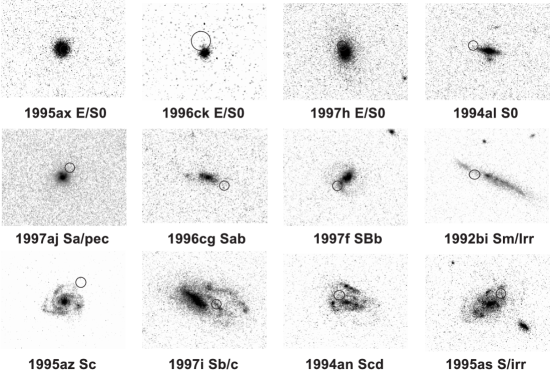
Figure 1: A selection of the SNe Ia host galaxies imaged using STIS on the HST, demonstrating the range of galaxy types and the quality of data produced by the program. In each image, the circle indicates the location of the (faded) SN derived via comparisons with existing ground-based data.

In the case of the STIS data, each targeted galaxy was imaged in the 50CCD (clear aperture) mode, which approximates a broad $V+R+I$ band-pass, in a $3\times 434\,\mathrm{s}$ dithered series. Basic image processing (bias subtraction, dark subtraction and flat-fielding) was performed using the standard STIS reduction pipeline from within iraf. Cosmic ray removal and final image construction was then performed using a ‘variable pixel linear-reconstruction’ technique using the dither-ii and drizzle packages (Fruchter & Hook, 1997). The output pixel size from this process was $0.025$ arcsec across, and a value $\mathrm{pixfrac}=0.6$ was used.

As well as this dedicated STIS snapshot program, we use WFPC-2 data for one host from another SCP HST program (ID:7590, PI: Perlmutter), and also searched the HST archive for additional HST observations of the hosts, finding three cases independently observed by HST/WFPC-2 (see Table 1 and references in P97 and P99). The WFPC-2 data sets were again combined using the dither-ii package used to reduce the STIS data.

The location of the faded SNe cannot be predicted with certainty on the HST (in particular STIS) images due to the pointing uncertainties generic in snapshot observations. In some cases where more than one galaxy is located near the centre of the HST pointing, this could confuse the correct assignment of the host galaxy. To accurately locate the position of the SNe on the HST (STIS or WFPC-2) images therefore requires careful comparisons with existing ground-based data taken in good seeing conditions. We performed a cross-correlation between the HST images and the existing calibrated ground-based images (cf. Aldering et al., in prep.). In these images, the SNe are visible, and hence the exact position can be determined in relation to surrounding objects. For the STIS field-of-view of approximately $52\arcsec\times 52\arcsec$, typically $6-8$ compact stellar-like objects were common to both the deep ground-based and the STIS data. We calculate the relationship between the HST and ground-based pixel coordinate systems using geomap and related tasks within iraf, and are then able to transform the pixel position of the SNe from the ground-based coordinate systems to the HST frame of reference.

We estimate the uncertainties in the derived positions using a simple ‘bootstrap’ technique. We calculate the location of the SN using all the common objects, and then perform the same calculation but omitting one common object each time. The resultant variation in the calculated location of the SN gives approximate uncertainties in the derived location using all the common objects. The process typically provides SN positions which are accurate to $\simeq 0.15$ – $0.4$ arcsec; the uncertainty is dependent on the number of objects in common between the two images and the seeing of the ground-based data. This accuracy is, in all cases, sufficiently precise to unambiguously identify the host galaxy.

This identification technique also enables us to derive projected radial distances from the SNe locations to the centre of their host galaxies for a sub-sample of the SNe. The use of spatially resolved HST images has the advantage of being able to precisely locate the centre of each galaxy reliably, something which is more difficult when using ground-based images. The uncertainty therefore derives entirely from the accuracy to which we can locate the SN position. In 20 of the 36 SNe with morphological information from HST images, we are able to calculate the SN location to an accuracy of $<0.3$ arcsec; these data will be discussed further in a later article.

We convert these distances in arcseconds to projected distances in kpc using the angular diameter–distance relation; where necessary in these calculations we assume a $\Omega_{\mathrm{M}}=0.28,\Omega_{\Lambda}=0.72$ and $H_{0}=70\,\mathrm{km\,s^{-1}\,Mpc^{-1}}$ cosmology.

3.2 Keck spectroscopy

The pre-existing ‘discovery’ host galaxy spectra were taken during the period when the SN light dominated that of the host galaxy. The principal goal of those spectroscopic campaigns was to determine a precise type and redshift for the SN candidate. As galaxies typically have narrow emission and absorption line features, their presence can often be detected even at maximum SN light; however, the contamination by the SN usually makes any detailed study of the host galaxy properties very difficult. We have therefore performed a second round of optical spectroscopy for a sub-sample of the host galaxies imaged by HST using the Echellette Spectrograph and Imager (ESI) on the Keck-II 10 m telescope (details on ESI can be found in Sheinis et al., 2002). The goal of this component is to considerably improve the diagnostic spectroscopy for the host galaxies.

ESI can operate in three observing modes (imaging, low dispersion and echellette); each galaxy was observed in the echellette and imaging configurations. The echellette mode has a continuous wavelength coverage of $\simeq 4000$ – 11000 Å, spread across ten orders with a constant $11.4\,\mathrm{km}\,\mathrm{s}^{-1}\,\mathrm{pixel}^{-1}$ dispersion. All spectroscopic observations were performed using a slit of width 1 arcsec. The position angle was calculated from the HST images to ensure the slit passes through both the location of the (now faded) SN and the host galaxy centre. Table 2 contains a log of the observations.

Table 2: The ground-based observing log for the new data on the host galaxies of the SCP high-redshift SNe.

SN Name	Spectroscopic	Spectroscopic	Imaging	Imaging data
	observation date	exposure time (s)	observation date	source
1992bi	2001 May 21	$2\times 1200$	2001 May 21	ESI
1994g	2000 Feb 10	$3\times 1200$	2000 Feb 10	ESI
1994al	2000 Nov 24	$2\times 1800$	2000 Oct 31	COSMIC
1994an	2000 Nov 24	$2\times 1800$	…	…
1995ar	2001 Nov 13	$2\times 1800$	…	…
1995az	2001 Oct 20	$2\times 1500$	2000 Oct 31	COSMIC
1995ax	2000 Nov 22	$2\times 1800$	2000 Oct 31	COSMIC
1996cg	2000 Feb 10	$3\times 1200$	2000 Feb 11	ESI
1997i	2000 Feb 10	$2\times 1200$	2000 Feb 10	ESI
1997h	2001 Oct 23	$2\times 1500$	…	…
1997f	2000 Feb 11	$3\times 1200$	2000 Feb 10	ESI
1997aj	2001 May 22	$2\times 1200$	2001 May 22	ESI
1997g	…	…	2000 Feb 10	ESI

The primary data reduction steps were performed using the makee data reduction software package written by T. Barlow. This package produces a bias subtracted, flat-fielded, wavelength calibrated and sky subtracted, but not order-combined, spectrum of each object by using a master trace of a bright star and shifting this trace to the position of the object to be extracted. A master bias frame and internal (quartz lamp) flat-field were created on every night of observation and used for that nights data; the wavelength calibrations were performed using HgNeXe and CuAr lamps bracketing each science observation.

On occasion, the automatic profile locating routine in makee failed for some orders or for those host galaxies which were spatially resolved. In these cases, the object profile location on the slit and the profile width were determined by hand and the spectrum extracted with these parameters.

In order to combine the ten orders into a single continuous spectrum, we performed flux calibration of the makee-extracted spectra using standard iraf routines using a flux standard observed on the night of observation at a similar airmass to the science target; suitable standards were drawn from the lists of Massey et al. (1988) and Massey & Gronwall (1990). We also correct for the extinction properties of the Mauna Kea summit atmosphere (e.g. Krisciunas et al., 1987; Krisciunas, 1990). Though an absolute flux calibration is not possible with a slit of finite width, a relative flux calibration between spectral regions is more reliable. The primary uncertainty here arises from variations in the seeing as a function of wavelength, where the FWHM of an image varies as $\lambda^{-1/5}$. We estimate the effect to be at the $\sim 5$ per cent level between H$\alpha$ and H$\beta$, the primary emission lines that interest us in this analysis.

After flux calibration, each order was examined and the wavelength range offering the best signal-to-noise (S/N) determined. These wavelength ranges were then median combined to form a final flux-calibrated spectrum from each individual exposure, and finally the individual exposures median combined to form a final output spectrum for each object.

Figure 2: Example spectra taken from the ESI spectroscopic campaign demonstrating the range of spectral types and the quality of the ESI data obtained.

The spectra were examined using the splot facility in iraf. For each output spectrum a redshift was measured via visual inspection, typically using Ca ii H,K absorption or [O ii]/Balmer emission-line features. We find excellent agreement with the earlier redshifts reported in P97/P99 in all cases. Fig. 2 demonstrates a range of the host galaxy spectra observed; comments on each spectrum can be found in Table 3. For the emission line spectra, we also attempt to measure the strength of the H$\alpha$ and H$\beta$ emission lines, where they are present and are not contaminated by poor residual sky subtraction from strong sky lines. These measures were also made using splot.

The H$\alpha$ and H$\beta$ lines give an indication of the extinction in a host galaxy, as the reddening nature of the dust makes the observed ratio of the fluxes of two emission lines ($R_{\mathrm{obs}}$) differ from the intrinsic ratio ($R_{\mathrm{int}}$). The colour excess of the ionised gas, $E(B-V)_{\mathrm{g}}$, can then be estimated via

$$E(B-V)_{\mathrm{g}}=\frac{\log(R_{\mathrm{obs}}/R_{\mathrm{int}})}{0.4[k(\lambda_{\mathrm{H}{\beta}})-k(\lambda_{\mathrm{H}{\alpha}})]}$$ (2)

where $k(\lambda)$ is the form of the total-to-selective extinction of the gas for a particular extinction law, and $\lambda_{\mathrm{H}{\beta}}$ and $\lambda_{\mathrm{H}{\alpha}}$ are the rest-frame emission wavelengths of H$\beta$ and H$\alpha$ respectively. Assuming case-B recombination, $R_{\mathrm{int}}=2.87$ for $\mathrm{H}{\alpha}/\mathrm{H}{\beta}$ (e.g. Osterbrock, 1989). The reddening parameter $A_{V}$ can be calculated via $A_{V}=E(B-V)_{g}R_{V}$, where $R_{V}\simeq 3.1$ for a Milky Way-type extinction law (e.g. Cardelli et al., 1989; Pei, 1992). Where available, these $A_{V}$ parameters are also listed in Table 3; also listed are values where the extinction due to the Milky-Way has been removed. These $A_{V}$ parameters have been corrected for stellar absorption affecting the H$\alpha$ and H$\beta$ lines assuming stellar absorption equivalent widths of 2Å in absorption on each. We make no corrections for the seeing variations between the two wavelengths of interest, but note that as seeing typically improves with wavelength (and hence slit losses will be smaller), our measured H$\alpha$ to H$\beta$ ratios will effectively be upper limits on the intrinsic ratios.

One further subtlety is that these values of $A_{V}$ are measured for the extinction on the nebular emission lines originating in star-forming H ii regions. This may not, and indeed probably will not, be representative for regions of the galaxy containing older stellar populations where SN Ia may originate; indeed, it has been shown that the continuum emission from stars in starburst galaxies is often less obscured than the line emission from the gas (e.g. Fanelli et al., 1988; Calzetti et al., 1994; Mas-Hesse & Kunth, 1999). An estimate of this extinction can be derived using the prescription of Calzetti et al. (2000), who relate the colour excess of the stellar continuum, $E(B-V)_{\mathrm{s}}$, to $E(B-V)_{\mathrm{g}}$ using $E(B-V)_{\mathrm{s}}=0.44\,E(B-V)_{\mathrm{g}}$.

We discuss the utility of the spectroscopic data further in Sections 4 and 6.

3.3 Ground-based Imaging

Many of the original SN search images detect the host galaxy, and photometric measures of these hosts are described and analysed in a companion paper which includes the reference and late-time images free from SN contamination (Aldering et al., in prep). As ESI offers an direct imaging capability, we took the opportunity to gather additional photometric measures when undertaking the spectroscopic component described above. Additional photometry was obtained with the COSMIC instrument at the Hale 200-in telescope at the Palomar Observatory. An observing log of all the new imaging observations obtained in addition to that described in Aldering et al. is given in Table 2.

The galaxies were observed in filters which most closely matched those filters used in the original SNe search program and in Aldering et al., the standard Cousins $R$ and $I$ band filters (corresponding to rest-frame bands $B$ and $V$ for most of our sample). In the case of ESI we used standard $R$ and Gunn $i$ filters (Thuan & Gunn, 1976), and for COSMIC we used Gunn $r$ and $i$. The new imaging data were reduced using standard techniques: overscan subtraction, bias subtraction and flat-fielding were performed using calibration data taken on the night of observation. The target host galaxy was identified using the original SN detection images, and raw magnitudes measured using the sextractor program version 2.21 (Bertin & Arnouts, 1996). We used the automatic aperture magnitudes determined by sextractor, which are similar to Kron’s ‘first moment’ algorithm (Kron, 1980). As the $R$ and $I$ images were taken consecutively on each night of observation, variations in the seeing between the $R$ and $I$ band data are negligible.

All the imaging data were taken on photometric nights and standard star fields (Landolt, 1992; Jorgensen, 1994) were observed at various airmasses to derive the CCD zeropoints and variation of extinction with airmass in order to calibrate the observed raw magnitudes on to the $\alpha$-Lyrae system. Finally, each integrated magnitude was corrected for galactic extinction using the colour excess maps of Schlegel et al. (1998).

Seven of the 11 host galaxies imaged with ESI $R$-band filter overlapped with the sample of Aldering et al., enabling us to determine the photometric precision of the joint dataset. We directly compare the $R$-band magnitudes derived from the two datasets, and find an excellent agreement; the mean absolute difference between the two datasets is only 0.06 mag (in the sense that the ESI magnitudes are fainter), with the largest discrepancy 0.12 mag. This discrepancy arises principally from the different magnitudes measured: Aldering et al. define their magnitudes to include all the light from within two Petrosian radii of a galaxy, whilst the definition of the magnitudes in sextractor leads to a slightly smaller aperture. These differing definitions will not affect the calculated colours unless the galaxies under study have marked colour gradients in their outermost regions. In the future analyses in this paper where we use these colours to help classify the hosts galaxies, we use data in the preference: i) Keck-ESI $R$,$i$, ii) Cousins $R$,$I$ (Aldering et al, in prep.), and iii) COSMIC $r$,$i$.

4 Host Galaxy Classification

We now turn to the question of characterising each host galaxy according to the data presented above. In the case of the high redshift SNe, we classified each host galaxy according to one of three broad categories: spheroidal (E/S0, type 0), early-type spiral (Sa through Sbc, type 1) and late-type spiral (Scd through to irregular types, type 2), based on a combination of the three diagnostics available to us.

In order of preference in the classification scheme, these are:

• HST morphology. The morphologies of the galaxies were visually classified by two of the authors (RSE and MS). The morphology of each HST-observed host is given in Table 1; examples of each classification can be found in Fig. 1.

• Ground-based spectrum. The ESI spectrum (or if not available a pre-existing SN discovery spectrum with sufficient S/N) was classified according to the presence or absence of nebular emission lines and the prominence of the discontinuity around Ca ii H and K. Our scheme runs from 0 (no emission lines, strong break) to 2 (clear strong H ii-like spectrum, no break). Comments on each object can be found in Table 3; example spectra are shown in Fig. 2.

• Ground-based integrated colour. We use a set of template SEDs (taken from Poggianti, 1997) to estimate the approximate galaxy class based on the observed $R$-$I$ colour and known redshift. The appropriate $R$ (or $r$) and $I$ (or $i$) filter response curves are convolved with each SED template at the host redshift, with the galaxy assigned a ‘colour–type’ based on the nearest matching galaxy SED. We do not account for redshift evolution in the galaxy SEDs in this process.

Table 3: ESI ground-based spectral classification

SN Host	Spectral type	$A_{V}$(raw)b	$A_{V}$(corrected)c	Commentsa
1992bi	2	0.11	0.06 (0.03)	Broad [O ii], H$\beta$, [O iii]
1994g	2	0.64	0.62 (0.27)	s. [O ii], H$\beta$, [O iii]
1994al	0	-	-	s. H,K, B4000
1994an	2	1.08	0.87 (0.38)	[O ii], H$\beta$, [O iii], H$\alpha$
1995ar	1	-	-	H,K, B4000, [O ii], H$\beta$
1995az	1	3.71	3.16 (1.39)	[O ii], H$\beta$, H$\alpha$
1995ax	0	-	-	Flat; w. H,K, B4000
1996cg	1	-	-	w. [O ii]
1997i	1	1.15	1.01 (0.44)	s. [O ii], H$\beta$, [O iii], H$\alpha$
1997h	0	-	-	s. H,K, B4000
1997f	1	-	-	w. [O ii], H$\beta$, [O iii]
1997aj	1	-	-	[O ii], H$\beta$, [O iii]

The question now arises as to how to combine these classifications, recalling that not all diagnostics are available for each host galaxy. We assigned a confidence of either 0 (probable) or 1 (secure), based on the agreement and availability of the various measures. This leads to two different samples of data – a ‘securely’ classified sample (our primary analysis dataset) and a slightly enlarged, but less securely classified, sample. Note that even in the less secure sample, the discrimination between spheroidal and disc based systems is usually robust, even if the precise class in the case of spiral systems is not clear. The following scheme is used:

• The HST imaging and ESI spectra; in all available cases these agree (Confidence ‘1’),

• Clear HST morphology; no ESI spectrum (Confidence ‘1’),

• Ambiguous HST morphology; supporting evidence from pre-existing (SN discovery run) spectral type or colour (Confidence ‘1’),

36 host galaxies (86 per cent of the total of 42 SNe in the P99 high-redshift sample) meet the above criteria. Three additional galaxies have been less securely classified according to:

• No HST image; class taken from good quality ground-based imaging and spectroscopic data (Confidence ‘0’).

• No HST image; class taken from good quality ground-based imaging or spectroscopic data (Confidence ‘0’).

In total we therefore have 39 classified galaxies in the enlarged sample (93 per cent of the total P99 high-redshift objects). The classification statistics can be found in Table 5 and the agreement between the different assigned types for the hosts can be examined in Fig. 3 in the context of the adopted ($R-I$) colour-redshift relation for those galaxies for which $R$ and $I$-band measures are available. The classifications are colour coded from red (E/S0) through green (early spiral) to blue (late spiral/irregular); black denotes those galaxies with no assigned class; these data can also be found in Table 4.

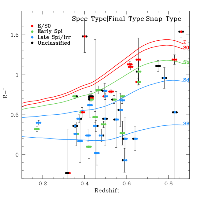
Figure 3: The colour-redshift relation for the subset of SN host galaxies with both $R$ and $I$ measures, together with the classification of the SN host galaxies from the three diagnostics available (the colour type, HST-type and spectral type). The colour shown is Galactic extinction corrected $R$-$I$; galaxies with colours measured based on Gunn filters are not shown (though similar diagrams exist for these smaller subsets). The final adopted classification is also shown. Overlaid SEDs are from Poggianti (1997), ranging from elliptical (E) to starburst (SB) galaxies. In the classification process, no redshift evolution in the galaxy properties is assumed to occur. Internal extinction in the host galaxies is not accounted for on this plot.

Table 4: The classification of the P99 42 high-redshift SN host galaxies

SN namea		Redshift	ESI STb	Other STb	Colour	HST	Final	Classification
					Type	Type	Type	security
1992bi		0.458	2	1	2	2	2	1
1994al		0.420	0	0	-	0	0	1
1994h	$\ast$	0.374	-	0	-	1	1	1
1994an		0.378	2	2	2	2	2	1
1994am		0.372	-	0	-	0	0	1
1994g		0.425	2	2	1	2	2	1
1994f		0.354	-	1	1	-	1	1
1995aq		0.453	-	2	2	-	2	1
1995ar		0.465	1	-	1	1	1	1
1995az		0.450	1	1	2	1	1	1
1995ay		0.480	-	2	2	-	2	1
1995at		0.655	-	0	1	1	1	1
1995ba		0.388	-	1	2	0	0	1
1995ax		0.615	0	0	1	0	0	1
1995aw		0.400	-	-	0	-	0	0
1995as		0.498	-	0	1	2	2	1
1996cg	$\ast$	0.490	1	-	2	1	1	1
1996cf		0.570	-	-	2	2	2	1
1996ci		0.495	-	-	1	2	2	1
1996cm		0.450	-	-	2	-	2	0
1996cl		0.828	-	0	1	0	0	1
1996ck		0.656	-	0	1	0	0	1
1996cn	$\ast$	0.430	-	-	1	1	1	1
1997i		0.172	1	1	2	1	1	1
1997h		0.526	0	0	1	0	0	1
1997g		0.763	-	-	2	2	2	1
1997f		0.580	1	1	2	1	1	1
1997j		0.619	-	0	1	0	0	1
1997l		0.550	-	-	2	2	2	1
1997o	$\ast$	0.374	-	2	2	-	2	1
1997p		0.472	-	1	1	-	1	1
1997s		0.612	-	2	-	-	-	-
1997n		0.180	-	2	2	2	2	1
1997q		0.430	-	-	1	0	0	1
1997k		0.592	-	-	2	2	2	1
1997r		0.657	-	-	1	1	1	1
1997ac		0.320	-	-	2	0	-	-
1997aj		0.581	1	1	2	1	1	1
1997ai		0.450	-	-	-	-	-	-
1997af		0.579	-	2	2	2	2	1
1997am		0.416	-	2	2	2	2	1
1997ap		0.830	-	-	2	-	2	0

Table 5: Statistics on the classification of the P99 42 high-redshift plus the extended low-redshift sample SN host galaxies

Host type	Low redshifta	High redshifta		Totala
		Secure	All	Secure	All
E/S0	3 ( 5)	9 ( 9)	10 (10)	12 (14)	13 (15)
Early Spi	14 (14)	9 (12)	9 (12)	23 (26)	23 (26)
Late types	8 ( 8)	14 (15)	16 (17)	22 (23)	24 (25)
Small Distances	14 (14)	- -	19 (19)	- -	33 (33)
Large Distances	10 (12)	- -	7 ( 7)	- -	17 (19)
All	25 (27)	32 (36)	35 (39)	57 (63)	60 (66)

As noted, the classifications of each object using the different techniques agree well; in particular, there are no red objects with emission line spectra or spiral morphology and no blue objects without emission lines which have a spheroidal HST-type. The greatest difficulty is in distinguishing between type 1 and type 2 objects, where the $R-I$ colour is of only limited value, possibly due to the increased presence of dust or evolutionary effects in these spiral systems when compared to E/S0 objects; in these objects we mostly rely on the other two diagnostics. Thus it is important to recognise the most robust distinction in our survey lies between type 0 and the remainder.

Classifications for the low-redshift SN host galaxy sample are taken from Hamuy et al. (2000). These authors give more than adequate morphological classes for all of the SNe in the low-redshift sample, and we simplify their system into the same three broader classes that we use for the higher redshift sample. Additional data on the projected distance (in arcsec) from the host galaxy is taken from Ivanov et al. (2000), which we convert into a projected distance in kpc.

One potential concern with the consistency of the morphological typing might be a mismatch between the filters used for the imaging at low and high redshifts – a morphological $k$-correction. However, the breadth of the STIS filter in use should minimize this effect. The low-redshift sample is typically typed using $B$ or $V$-band images (see Hamuy et al., 2000), which at the mean redshift of our high-redshift sample would correspond to a $R$ or $I$ passband, which falls within the $V+R+I$ response of the STIS 50CCD; indeed this was one of the motivations for selecting the broad 50CCD observing mode.

5 Results

With each galaxy classified according to its morphological or spectral type, we now search for any environmental effects that may be present in the combined sample of high and low redshift SNe. This section presents our results in two broad categories. Firstly, we examine the Hubble diagram and its associated statistics as a function of the environment of the SN, both in terms of the host galaxy morphology and galactocentric distance. Secondly, we investigate possible correlations between the light curve parameters of the SNe and its environment similarly characterised. We discuss the broader implications of our findings in Section 6.

5.1 Hubble diagrams as a function of SN environment

We first examine the updated P99 Hubble diagram (fig. 2 in P99), labelling each SN according to its host galaxy type. The upper panel of Fig. 4 shows this Hubble diagram in terms of the effective rest-frame $B$ magnitude, i.e. corrected for the light-curve stretch-luminosity relationship of equation (1), as a function of redshift for the 42 SCP high-redshift SNe, together with the 25 SNe from the low-z C-T/CfA samples. A zoom to the high redshift sample is also shown. Those SNe excluded from the primary fit of P99 are marked.

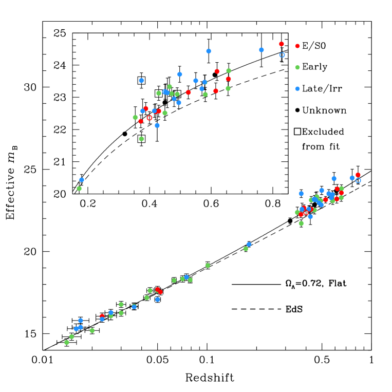
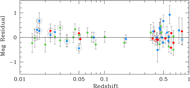
Figure 4: UPPER PANEL: The stretch-corrected SNe Ia Hubble diagram plotted according to the class of the host galaxy. The inset shows the high-redshift SNe, the main panel the Hubble diagram for the entire sample. Boxed points show high-redshift SNe excluded from the P99 solution. LOWER PANEL: The residuals from the adopted cosmology (‘fit-C’ of P99) for both high and low-redshift SNe. Excluded SNe are not plotted. Dotted-circled points discriminate between CfA SNe and C-T SNe. In both panels unfilled circles denote galaxies with a less secure type-classification.

The SNe are colour-coded according to the host galaxy class. Less-securely classified hosts are also marked. Those SNe with no classes are marked unknown and ignored in the subsequent analyses. The overlaid lines correspond to the apparent magnitude as a function of redshift for a standard $s=1$ SN Ia expected in an EdS Universe ($\Omega_{\mathrm{M}}=1$, $\Omega_{\Lambda}=0$) and a flat, $\Lambda$-dominated Universe with the best-fitting cosmology of P99 ($\Omega_{\mathrm{M}}=0.28$, $\Omega_{\Lambda}=0.72$; see P99, also Riess et al., 1998). The lower panel in Fig. 4 shows the residuals from this best-fitting line for each SN.

We also perform additional fitting procedures for the SNe residing in each galaxy class using a technique similar to that used in P99. We consider two cases – fitting for both $\Omega_{\mathrm{M}}$ and $\Omega_{\Lambda}$ independently, and fitting for the case of a flat Universe (i.e. fitting only for $\Omega_{\mathrm{M}}$ or $\Omega_{\Lambda}$ and assuming $\Omega_{\mathrm{M}}+\Omega_{\Lambda}=1$). This involves solving the equation

$$m_{B}^{\mathrm{corr}}=m_{B}^{\mathrm{raw}}+\alpha(s-1)={\cal M}_{B}+5\log D_{L}(z;\Omega_{\mathrm{M}},\Omega_{\Lambda}),$$ (3)

where ${\cal D}_{L}\equiv H_{0}\,d_{\mathrm{l}}$ is the ‘Hubble-constant free’ luminosity distance, and ${\cal M}_{B}\equiv M_{B}-5\log H_{0}+25$ is the ‘Hubble-constant-free’ $B$-band absolute peak magnitude of a SN Ia with $s=1$ (see e.g. Goobar & Perlmutter, 1995, and P99). This equation is solved for the parameters $\alpha$, ${\cal M}_{B}$, $\Omega_{\mathrm{M}}$ and, for non-flat geometries, $\Omega_{\Lambda}$, by least-squares i.e. minimizing

$$\chi^{2}\left(\Omega_{\mathrm{M}},\Omega_{\Lambda},\alpha,{\cal M}_{B}\right)=$$ (4)

$$\sum^{N}_{i=1}\frac{\left(m_{Bi}^{\mathrm{raw}}-\left[{\cal M}_{B}+5\log D_{L}\left(z_{i}\right)-\alpha\left(s_{i}-1\right)\right]\right)^{2}}{\sigma_{i}^{2}}.$$

As in P97 and P99, the small correlations between the high-redshift SNe (due to shared calibration data) are accounted for using a correlation matrix of the various uncertainties. We compare two numerical minimization techniques: a simple Levenberg-Marquardt technique, and a more complex Gauss-Newton method, and find an excellent agreement between the derived parameters in both cases.

Details of the best-fitting parameters are given in Table 6. The table also includes the fit obtained for all of the SNe with a host galaxy type (regardless of class) which provides a valuable consistency check that our ‘typed’ sample is representative of the larger one studied by P99. The parameters $\alpha$ and ${\cal M}_{B}$ are determined only for the P99 SNe sample and for the new enlarged sample, and the parameters from the latter fit adopted as fixed in the smaller sub-samples. (We study variations in ${\cal M}_{B}$ in detail in Section 6, whilst the $\alpha$ parameter has only a small impact at high-redshift due to the narrow stretch distribution seen, e.g. fig. 4 in P99). For these fits, the errors in the best-fitting $\alpha$ and ${\cal M}_{B}$ parameters are carried through in the analysis. For a flat $\Omega_{\mathrm{k}}=0$ Universe, Table 6 also lists the mean dispersions from the best-fitting cosmologies for each sample, as well as formal 1-$\sigma$ errors in $\Omega_{\mathrm{M}}$ derived from the co-variance matrices of the various fits, assuming normally distributed errors. The fitting procedure also generates two-dimensional confidence regions, ${\cal P}(\Omega_{\mathrm{M}},\Omega_{\Lambda})\propto\exp(-\chi^{2}/2)$, shown in Fig. 5 for a selection of the SN sub-samples. The plot shows the 68% and 90% confidence ellipses in the ($\Omega_{\mathrm{M}}$, $\Omega_{\Lambda}$) plane together with the best-fitting parameters for general and flat cosmologies. For those datasets where $\alpha$ and ${\cal M}_{B}$ are fit, as in P99 we calculate two-dimensional confidence regions by integrating over these parameters, i.e., ${\cal P}(\Omega_{\mathrm{M}},\Omega_{\Lambda})=\int\int{\cal P}(\Omega_{\mathrm{M}},\Omega_{\Lambda},{\cal M}_{B},\alpha)\,\mathrm{d}{\cal M_{B}}\,\mathrm{d}\alpha$. This probability space also allows us to estimate upper and lower error bounds on $\Omega_{\mathrm{M}}$ separately, which we also report in Table 6.

Figure 5: Confidence regions in ($\Omega_{\mathrm{M}}$, $\Omega_{\Lambda}$) for the fitting procedures in the different sub-samples listed in Table 6. The ellipses correspond to 68 and 90% confidence regions, and the best-fitting cosmologies are denoted by a filled diamond (general cosmology) and a filled circle (flat cosmology). The diagonal line corresponds to a flat Universe, the dotted line shows the boundary between ‘no big-bang’ models, the dashed line denotes the infinite expansion boundary, and the dot-dashed line denotes those Universes which are currently undergoing acceleration. For those fits where $\alpha$ and ${\cal M}_{B}$ were fit (panels A and B), the confidence regions are obtained by integrating over these parameters (see text for details).

The probability distributions also allow us to calculate the probability that $\Omega_{\Lambda}>0$ and the probability that the Universe is currently accelerating in its expansion for each SN sub-sample. The latter can be expressed via the current, $z=0$, deceleration parameter, $q_{0}$, where $q_{0}=\frac{\Omega_{\mathrm{M}}}{2}-\Omega_{\Lambda}$. As negative values of $q_{0}$ indicate deceleration at the current epoch, the condition for current acceleration in the expansion of the Universe is given by

$$\Omega_{\Lambda}>\frac{\Omega_{\mathrm{M}}}{2}.$$ (5)

The probabilities for these two classes of cosmological model are also listed in Table 6.

We also investigated potential environmental dependencies in the SN properties by plotting the Hubble diagram with each SN labelled according to its projected galactocentric distance (Fig. 7). SNe located at less then 7.5 kpc (the approximate mean of the sample, as well as the value used in the analysis of Wang et al., 1997) from the galaxy centre are shown in red, those at larger distances are in blue. We also fit these two additional subsets of SNe using the same procedure as above; the results of these fits are again in Table 6.

Table 6: The best-fitting cosmologies for SNe residing in each of the host galaxy types.

SNe Subset	Median	Best ($\Omega_{\mathrm{M}}$,$\Omega_{\Lambda}$)	Best $\Omega_{\Lambda}$b	Monte-Carlo	Mean	DOFd	$\chi^{2}$	$\chi^{2}$	Probability that:
	redshifta			‘error’	dispersionc			/DOFd	$\Omega_{\Lambda}>0$	$\Omega_{\Lambda}\geq\frac{\Omega_{\mathrm{M}}}{2}$
Fits with all parameters free:
P99 ‘fit-C’	0.476	0.73, 1.32	$0.72^{+0.09}_{-0.08}$	$\pm 0.07$	0.199 (0.199)	51	57	1.121	99.79	99.59
P99 + CfA	0.476	0.37, 0.67	$0.65^{+0.11}_{-0.09}$	$\pm 0.06$	0.216 (0.214)	60	82	1.376	98.24	97.30
Typed SNe	0.480	0.46, 0.77	$0.64\,(0.64)^{+0.11}_{-0.10}$	$\pm 0.07$	0.223 (0.221)	59	81	1.388	97.96	96.84
Fits with $\alpha$ and ${\cal M}_{B}$ fixed:
E/S0	0.478	0.83, 1.02	$0.57\,(0.58)^{+0.12}_{-0.11}$	$\pm 0.09$	0.159 (0.173)	12	8	0.680	97.09	94.80
Spirals	0.480	0.44, 0.81	$0.67\,(0.66)^{+0.07}_{-0.06}$	$\pm 0.09$	0.235 (0.234)	46	73	1.590	99.85	99.75
Early	0.472	0.62, 0.65	$0.50\,(0.50)^{+0.12}_{-0.11}$	$\pm 0.14$	0.200 (0.193)	22	28	1.309	92.46	86.83
Late	0.487	0.45, 1.03	$0.77\,(0.78)^{+0.08}_{-0.07}$	$\pm 0.09$	0.272 (0.274)	23	40	1.761	99.98	99.97
Large Distance	0.458	0.72, 0.80	$0.53^{+0.16}_{-0.14}$	$\pm 0.14$	0.196 (0.204)	15	19	1.276	94.38	89.46
Small Distance	0.498	0.77, 1.13	$0.65^{+0.08}_{-0.08}$	$\pm 0.11$	0.256 (0.251)	32	56	1.777	99.57	99.27

We checked the reliability of our quoted uncertainties in $\Omega_{\Lambda}$ (derived from the co-variance matrices of the various fits) by performing detailed Monte-Carlo simulations of each SN data sub-set. We created 10000 artificial datasets for each of the 9 sub-samples (see Table 6) by drawing $N$ SNe at a time (with replacement) from the relevant sample, where $N$ is the number of SNe in each set. We then fit these $N$ SNe in the same way as for the original sample. The mean of the resulting distribution in each fitted parameter is satisfactorily close to the final fitted parameter of the original dataset, with the standard deviation of the distribution representing approximate 1-$\sigma$ uncertainties in the various fits. These Monte-Carlo estimated uncertainties are also listed in Table 6.

We now turn to examining the significance of the various correlations in the above plots. Fig. 4 and Table 6 reveal some interesting trends.

Firstly, each of the various samples and sub-samples strongly supports the SCP/HZT conclusions for the presence of a cosmological constant; indeed all sub-samples exclude an EdS Universe at greater than the 99 per cent confidence level and favour cosmological models with $\Omega_{\Lambda}>0$ with $>97$ per cent confidence. If we restrict ourselves to flat $\Omega_{\mathrm{k}}=0$ models, this confidence increases to $>99$ per cent for all SN sub-samples. Most noticeably, the scatter about the best-fitting line for SNe arising in spiral or irregular hosts is greater than that for SNe arising in spheroidal host galaxies (see also the $\chi^{2}$/DOF in Table 6). This trend of increased scatter with class is particularly striking and can be seen more clearly by examining the dispersions from the best-fitting cosmology (Fig. 6).

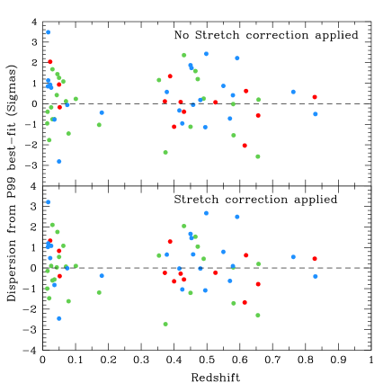
Figure 6: The dispersions (in sigmas) from the best-fitting cosmology of P99 (‘fit-C’) as a function of host galaxy type, for both peak magnitudes corrected for the light-curve-width-luminosity relation (bottom) and uncorrected magnitudes (top). The colour coding is as in Fig. 4.

If patchy dust extinction were the origin of the increased scatter in the later type hosts, we would expect, on average, the SNe in these systems to appear fainter. Such a trend is indeed seen; SNe occurring in spiral galaxies appear fainter, with or without the application of a stretch-correction. These conclusions are not affected if we only consider the securely classified sample of host galaxies (see Table 6). We will return to the significance of this conclusion in the next section.

The reduced scatter we observe for the E/S0 sample is an important result. Accordingly, we are interested in understanding whether it is a robust result. To verify this, we have performed simulations to determine how likely we would be to obtain similar sub-samples to the E/S0 sample by chance. We draw $N_{\mathrm{ell}}$ high-redshift SNe from the full sample (where $N_{\mathrm{ell}}$ is the number of high-redshift SNe in E/S0 galaxies) and perform the same best-fitting procedure to these SNe. By repeating the test a large number (10000) of times, we investigated how frequently the derived cosmological parameters produce a $\Omega_{\Lambda}$ smaller than the actual E/S0 sample and a smaller mean dispersion about the best-fitting cosmology.

Figure 7: As Fig. 4, but with the SNe plotted according to the projected location from the centre of the host galaxy. Stretch corrections are applied. Filled circles show SNe lying at $<7.5\,\mathrm{kpc}$, whilst empty circles show SNe at larger projected distances.

We find that less than 3 per cent of the random samples possess a $\Omega_{\Lambda}$ smaller than that found for E/S0 galaxies, and a mean dispersion about the best-fitting cosmology smaller than that for the E/S0 SNe. Thus it seems the E/S0 sample is unlikely to be simply a sub-sample selected randomly from the larger sample of SNe, and that there is a significant difference in the photometric properties of the E/S0 SNe that differs from the mean of the full SNe sample.

Finally, we can see no clear trends in the Hubble diagram plotted according to the projected distance of the SN from the host galaxy (Fig. 7), again regardless of whether stretch corrections are applied.

5.2 Correlations between light-curve parameters and environment

In studies of the environments of local SNe Ia, many authors (e.g. Riess et al., 1999; Hamuy et al., 2000) find that intrinsically brighter SNe (SNe with larger stretch values) occurred in late-type galaxies, and intrinsically fainter (small stretch) SNe were preferentially located in spheroidal hosts. It is important to ensure that the effects we see in Fig. 4 are not systematic effects simply related to the application stretch corrections which vary according to the type of the host galaxy (e.g. Hamuy et al., 2000).

We have considered this issue in two ways. First, we have repeated the cosmological fits of Section 5.1, comparing the dispersions from the best-fitting cosmology with and without applying the stretch corrections to each peak luminosity (Fig. 6). We find that the trends in Fig. 4 remain even if stretch corrections are not applied, with very similar derived cosmological parameters within the uncertainties quoted in Table 6.

More directly, we can examine the distribution of the stretch parameter for each SN located in each galaxy type. Fig. 8 shows this comparison for the high and low redshift samples. The trend noted by Riess et al. (1999) and Hamuy et al. (2000) is apparent in the low-redshift sample: an absence of small-stretch SNe in late-type galaxies and of large-stretch SNe in early-type galaxies . However, this same trend is not seen in the SCP high-redshift SNe sample. This is due to the fact that, as shown in P99 (their fig. 4), the stretch distribution of the high-redshift SNe is narrower than that seen in the low redshift samples. We return to this in Section 6.

Finally, Fig. 9 shows the SN stretch plotted as a function of projected distance from the host galaxy. Here a weak trend is found possibly suggesting that SNe at greater projected distances may be fainter, similar to that seen in the local sample of Riess et al. (1999). This could possibly arise if, within a distribution of luminosities, fainter SNe were systematically missed close to the galaxy core (e.g. Shaw, 1979), though sensitivity calculations on the high-redshift sample suggest this is unlikely to be the case (Pain et al., 1996, 2002).

Figure 8: The distribution of SN stretch with host galaxy type. The low-redshift SNe are taken from the Hamuy et al. (1996a) and Riess et al. (1999) samples; see text for further details. All SNe (including those rejected as stretch outliers from the cosmological fits) are shown in this figure.

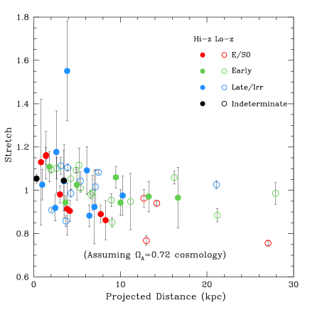
Figure 9: The SN stretch plotted as a function of projected distance from the centre of the host galaxy. The colour coding is as in Fig. 4.

6 Discussion

Of the various results presented in Section 5, the most robust and significant trend we have found is that SNe found in spiral and irregular galaxies present a larger scatter around the best-fitting cosmological model than those located in E/S0 galaxies. However, SNe in all galaxy types provide evidence for a significant cosmological constant (at $\simeq 5\sigma$). Additionally, SNe in late-type galaxies also appear fainter than those found in E/S0s, regardless of whether stretch-corrections are applied.

An obvious explanation of these main results, which do not depend on whether stretch corrections are made, is that there is increased extinction in later type galaxies and of an amount which varies somewhat from galaxy to galaxy. Though the SNe magnitudes are corrected for Galactic extinction, no account is taken of dust residing either in the host galaxy or along the line of sight.

P99 investigated the effect of differential reddening on the high-redshift SNe as compared to their local counterpart by contrasting the mean $B-V$ colour of high redshift SNe at maximum light with that for the local sample. They find that the colour excess distributions show no significant differences at low and high redshift, with the reddening distributions for the high-redshift objects consistent with the reddening distribution for low-redshift SNe within the measurement uncertainties, and both samples possessing almost identical error-weighted means. Additionally, they perform cosmological fits with each SN corrected for extinction according to its $E(B-V)$, and find that the fitted parameters change little with this modification.

In the following we have revisited and extended this analysis. Although the precision is poor for an individual SN, it is advantageous to re-examine the situation as we now have independent diagnostics which relate to the presence of host galaxy dust. The differential reddening affecting any one SN can be determined by comparing its observed $B_{\mathrm{max}}-V_{\mathrm{max}}$ with the $(B_{\mathrm{max}}-V_{\mathrm{max}})_{0}$ for low-redshift SNe with the same stretch-factor. The differential colour excess $E(B-V)$ is determined as

$$E(B-V)=(B_{\mathrm{max}}-V_{\mathrm{max}})_{\mathrm{obs}}-(B_{\mathrm{max}}-V_{\mathrm{max}})_{0}.$$ (6)

The $(B_{\mathrm{max}}-V_{\mathrm{max}})_{\mathrm{obs}}$ are calculated following P99. For SNe in the redshift range $0.3<z<0.7$, the $R$ and $I$ band measures are used instead of $B$ and $V$ and $(B_{\mathrm{max}}-V_{\mathrm{max}})_{\mathrm{obs}}$ is calculated using appropriate $k$-corrections (Kim, Goobar, & Perlmutter, 1996; Nugent, Kim, & Perlmutter, 2002). For SNe at $z>0.7$ the $R$ and $I$ measures correspond more closely to SN rest-frame $U$ and $B$ bands, so $E(B-V)$ is calculated from $E(U-B)$; likewise for SNe at $z<0.3$, where the $R$ and $I$ correspond to rest-frame $V$ and $R$, $E(B-V)$ is calculated from $E(V-R)$. We omit those 6 of the 42 high-redshift SNe that do not have both $R$ and $I$ measures from this analysis.

The distribution of this $E(B-V)$ parameter as a function of the host galaxy type is shown in Fig. 10. The errors in $E(B-V)$ are derived from the uncertainties in the $R$ and $I$ photometry. The error-weighted mean values of $E(B-V)$ for each class are -0.01, 0.20 and 0.03 for E/S0, early spirals and later spirals/irregulars respectively; the value for spirals taken as a whole is 0.10. We can see that SNe lying in E/S0 galaxies form a very narrow and tight distribution around a mean $E(B-V)\simeq 0$, whereas SNe residing in spiral galaxies show a larger range of $E(B-V)$ values and means of $E(B-V)>0$. This is suggestive that, as expected, SNe in E/S0 galaxies are unlikely to be affected by the presence of dust, whereas the effect of dust on SNe in spiral systems is more uncertain. Furthermore, the two SNe rejected from ‘fit-C’ in P99 as ‘likely-reddened’ (1996cg and 1996cn) are both located in early spiral galaxies; indeed, these two objects are the primary cause of the large mean value of $E(B-V)$ found for these systems.

Figure 10: The SN rest-frame ‘colour excess’ ($E(B-V)$) plotted as a function of the host galaxy type. $E(B-V)$ is as defined in the text (see also P99). The error-weighted mean of each distribution are shown as stars; the error bars are derived from the $R$ and $I$ photometry for each SN. The vertical offsets for each plotted SN is used to avoid over-plotting the data points and is illustrative only. Only the high-redshift SNe are shown.

The above result is, to some extent, independent of the morphological trends seen in the Hubble diagram since the former relies on the SN colour whereas the latter depends on the peak luminosity. Naturally there are possible inter-dependencies but we argue both results provide strong support for our two main conclusions. Firstly, much of the scatter in the SNe Ia Hubble diagram arises from extinction in the later type galaxies. As this scatter is host galaxy morphology-dependent, clearly it is internal to the host galaxies. Secondly, not only do we see a tight scatter in the Hubble diagram for SNe in E/S0s, but differentially there is no obvious difference in the extinction as inferred from the SNe at high and low redshift. Accordingly, the cosmological conclusions derived from this E/S0 subset must be particularly robust to systematic errors arising from extinction. As can be seen in Table 6, this data provides a $\simeq 5\sigma$ detection of a non-zero cosmological constant.

Table 7: The best-fitting ${\cal M}_{B}$ for SN Ia arising from different galaxy types, assuming the best-fitting cosmology for the E/S0 sub-sample.

	E/S0	Early Spi	Late Spi/Irr	All Spirals
${\cal M}_{B}$	$-3.39\pm 0.07$	$-3.37\pm 0.08$	$-3.25\pm 0.06$	$-3.32\pm 0.05$
Difference with E/S0 sample	–	$0.02\pm 0.11$	$0.14\pm 0.09$	$0.07\pm 0.09$

An interesting question then is: how much extinction in high-redshift SNe Ia is implied by our results? We can address this question in the following manner. We repeat our cosmological fits for the E/S0 and various spiral SNe sub-samples, but this time fit for the parameter ${\cal M}_{B}$ rather than $\Omega_{\mathrm{M}}$ and $\Omega_{\Lambda}$, and instead hold $\Omega_{\mathrm{M}}$ and $\Omega_{\Lambda}$ fixed at their values as derived from the (presumed dust-free) E/S0 sample of SNe. As ${\cal M}_{B}$ is the intrinsic $B$-band peak magnitude of a SN Ia, if those SNe in E/S0 galaxies are less affected by dust than those in spiral galaxies, we might expect the best-fitting ${\cal M}_{B}$ to be brighter in these galaxies. These best-fitting ${\cal M}_{B}$ values and 1-$\sigma$ errors are given in Table 7.

Assuming the best-fitting E/S0 flat-Universe cosmology, SNe appear $0.14\pm 0.09$ mag fainter in late-type spirals than in E/S0s. However, these uncertainties are currently large (due to the small number of objects in the different samples), and the result is consistent with both a near-zero offset and an offset of 0.23 mag. Though there are obvious caveats associated with this result, and the scatter from SN to SN is large due to the photometric uncertainties in the SN magnitudes, this measure would however appear to suggest that the amount of extinction suffered by these high-redshift objects is small, confirming earlier conclusions (e.g. P99).

This result appears in contradiction to the work of Rowan-Robinson (2002), who suggest that the evidence for a positive cosmological constant is reduced if an average internal dust-extinction correction of 0.33 mag for all high-redshift SNe is made. However, median extinction values as large as this do not appear consistent with these new results, particularly in the E/S0 systems where internal extinction is expected to be very small, and which show that $\Omega_{\Lambda}>0$ at $\simeq 5\sigma$.

Modest extinction for even the SNe occurring in late-type galaxies is supported by the small amount of spectral data available for the emission line host galaxies (Table 3), though the extinctions implied are not as small as those indicated by the dispersions in the Hubble diagram. For the 6 galaxies where a measure of the Balmer decrement is possible (all at $z<0.5$ due to H$\alpha$ shifted out of the ESI spectral coverage) the measures suggest (except for one case) small extinctions on the nebular emission lines, and hence smaller extinction on the stellar continuum likely affecting the observed SNe, using the prescription of Calzetti et al. (2000). However, most of the measured $A_{V}$ are still larger than the 0.14 mag implied by the difference in ${\cal M_{B}}$ between E/S0 and spiral systems (Table 7). We hypothesise this is due to SNe lying well away from the H ii regions from which the nebular lines used to measure the dust content originate, an effect which is not removed even after using the Calzetti et al. (2000) prescription. In the one case where the extinction measured is large ($A_{V}\simeq 3$, 1995az), the SN was located at a large projected galactocentric distance of $\sim 13\,\mathrm{kpc}$, one of the largest in the sample (see Fig.s 1 and 9), where the large amounts of dust that were detected in the H ii regions may not be present. Clearly larger samples of spectra are required to confirm these trends.

At first sight, the small extinction found for SNe in late-type galaxies appears a surprising result. Observational evidence suggests that the amount of star-formation in normal field galaxies increase with redshift (e.g Lilly et al., 1996), and that much of this increase results from late-type and irregular systems (Brinchmann et al., 1998), which presumably should be dustier systems than their non-starforming counterparts, as increased star-formation activity is usually associated with increased dust content. Although we see such a correlation in our data, in absolute terms the SNe of P99 even in the later-type hosts appear to suffer little extinction, as confirmed by the limited spectroscopic data presented here and the colours of the low and high-redshift SNe at maximum light.

Hatano et al. (1998) have investigated the effects of extinction on the optical properties of SNe. For simple assumptions concerning the spatial distribution of dust and SN progenitors in a model disc galaxy, they find that the amount of extinction suffered by SNe is small. The typical ranges in mean $A_{B}$ is 0.3 mag to $>1$ mag when all SNe are considered; however these means are dominated by a few high extinction events – most SNe are mildly obscured, but with a long tail to higher extinction events, which drop out of flux-limited surveys such as the SCP/HZT search campaigns. Mean values for an ‘extinction-limited subset’ ($A_{B}<0.60$) range from 0.12 to 0.16 mag, depending on the inclination of the system, in good agreement with the 0.14 mag difference we find between E/S0 and late-type spiral SNe.

A further explanation for the low extinction on high-redshift SNe in late-type systems is that the progenitors of SNe Ia are largely located in the outermost components of disc and irregular galaxies, perhaps as landmarks of earlier stages of galactic assembly, whereas the dust is distributed within regions of more recent star-formation activity confined to the thin disc. In popular hierarchical models, where the bulk of galactic assembly occurs over $1<z<3$, one would expect much mixing of dust and old stars. The absence of significant extinction in the bulk of our sample might be used to argue against a significant increase in the merger rate prior to $z\simeq 0.5-0.8$.

Another possible explanation is related to the selection effects inherent in SN Ia surveys; do SN Ia searches sample the entire range of galaxy types available at a given redshift? Alternatively, are we missing SNe that reside in particularly dusty host galaxies? In principle, we can examine this by comparing the morphological mix of our host galaxy sample to the observed mix of normal galaxies in the same redshift range. The most relevant study to date is that of Brinchmann et al. (1998), who analyse HST imaging of the galaxies selected in the CFRS and LDSS redshift surveys. They classify their sample into three broad classes – E/S0s, spirals and irregulars – and find a large increase with redshift in the fractional number of irregular objects from 9 per cent at $z<0.5$ to over 30 per cent at $0.7<z<0.9$, with decreases in the relative numbers of E/S0s and regular spirals. This leads to a change in the split of both integrated $B$-light luminosity density (see Brinchmann et al., 1998), and a change in the morphological split of integrated stellar mass density (see Brinchmann & Ellis, 2000), both likely related to SN Ia events. Hence, in a truly volume-limited survey of SNe Ia, we might expect the fraction of events found in irregular galaxies to sharply increase at $z>0.5$, tracing the increased stellar mass in these systems.

Comparisons with this study are obviously problematic due to the small size of the current sample and the differing redshift ranges, as well as differing classification techniques for the galaxies. We have 16 securely classified galaxies at $0.5<z<0.8$, of which 7 are classed as type-2 ($44\pm 17$ per cent). However, the Brinchmann et al. scheme would class many of these regular late-type galaxies separately from those which are irregular systems – only 3 of the objects ($19\pm 11$ per cent) are irregular in this definition scheme. Brinchmann et al. find a fraction of $33\pm 6$ per cent, opening the possibility that we do not see this same rapid rise in the number of ‘truly’ irregular systems in the SN sample.

This possible lack of irregular systems can be reconciled if we hypothesise that such objects contain, on average, larger amounts of dust due to their presumably higher star-formation activity. This would result in any SNe located in these galaxies to be dimmed to a greater extent than those in E/S0 or regular spiral systems; the SNe searches could therefore be (implicitly) biased against extincted SNe. Conceivably, many SNe Ia do suffer significant extinction but, because of the flux-limited SNe search criteria, they are not included in our sample.

Our observation that SNe Ia residing in E/S0 galaxies show a smaller scatter about the best-fitting cosmological model (as revealed by the $\chi^{2}$/DOF for the various fits in Table 6) allows us to estimate the intrinsic spread in the peak magnitude of these SNe compared to those residing in other classes of galaxy. Currently, each SNe error contains a contribution of 0.17 mag added in quadrature to allow for the uncertainty in the light-curve-width-luminosity correction (e.g. Hamuy et al., 1996b), regardless of the host class. As some of this dispersion arises from host galaxy extinction, we can use the (presumed) dust-free E/S0 SNe population to estimate the intrinsic dispersion for this class of SNe. For SNe in each host type, we therefore repeat the cosmological fits, altering the intrinsic dispersion until the $\chi^{2}$/DOF for each fit is equal to one. We perform this test for the high and low-redshift SNe taken together, and also solely for the high-redshift SNe.

The intrinsic dispersions are (in magnitudes) 0.09(0.10), 0.29(0.25), and 0.69(0.24) for E/S0, early and late-type spirals/irregulars respectively – bracketed values refer to fits where only high-redshift SNe are used (the values for spirals taken as a whole are 0.46 and 0.26) . Note that the small intrinsic dispersion seen for those SNe in E/S0 matches very closely the dispersion seen in low-redshift SNe after a technique correcting for the effects of reddening has been applied (0.11 mag; see Phillips et al., 1999), and the large dispersion seen in late-type spiral classes is heavily influenced by one or two low-redshift outliers. The implication from this small dataset is clear: SNe residing in E/S0 hosts are superior ‘standard candles’ than those in later-type galaxies due to the small amount of extinction affecting them.

Finally, it is important not to overlook a possibly important result suggested by the lack of range in light-curve width (or stretch) indicated in Fig. 8. This figure does provide some evidence of a shift in the population distribution between SNe found at low and high-redshift: at high-redshift we see no trend in stretch with galaxy type, whereas at low-redshift SNe with larger stretches are found in later-type galaxies and are missing from E/S0 galaxies. It’s important to emphasise that this population shift has no impact on the security of the cosmological results, as light-curve-width differences are accounted for in the stretch correction of equation (1), and stretch outliers are in any case rejected from the fits. Given the small number of SNe in each group, Fig. 8 will, of course, be sensitive to one or two extreme or unusual events. Bearing this caveat in mind, we performed Kolmogorov–Smirnov (K–S) tests on the different stretch distributions for SNe residing in each galaxy class, and find the significance levels for the hypothesis that the SNe at low and high-redshifts are drawn from different distributions to be 89, 71 and 7 per cent for E/S0, early- and late-type galaxies respectively (the significance level for low-redshift SNe in E/S0 and late-type galaxies having a different stretch distribution is 94 per cent in this sample). Though these trends are only suggestive given the small number of events, they might be explained if we assume that the light-curve properties of SNe Ia depend primarily on the age of the progenitor system.

At low redshift, it appears intrinsically fainter SNe are located in older (E/S0) stellar environments rather than young spiral systems (e.g. Hamuy et al., 2000). As we look to higher-redshift (i.e. viewing galaxies at an earlier stage in the evolution of their composite stellar populations), the E/S0 galaxies will posses younger populations than is the case in the local Universe (at $z=0.5$, the age of the Universe is $\sim 8\,\mathrm{Gyr}$ compared to $\sim 13\,\mathrm{Gyr}$ at $z=0$ in a $\Lambda$CDM cosmology). If, as was discussed in Section 1, older progenitors generate fainter SNe events, at high-redshift we would not expect to see the fainter (smaller stretch) SNe found in local, older, E/S0 galaxies (Hamuy et al., 2000), thus strengthening the case for a cosmological constant.

7 Conclusions

We have investigated the Hubble diagram of Type Ia supernovae spanning a large range in redshift and have classified 39 distant events according to the nature of their host galaxies as revealed by HST imaging, intermediate dispersion spectroscopy and broad band colour. Together with morphological data for the host galaxies of 25 local SNe drawn from the literature, we find the following.

1. The scatter on the SN Ia Hubble diagram, as determined from residuals of the peak brightness with respect to the best fit cosmological model, correlates closely with the host galaxy type. The scatter is minimal for SNe occurring in host galaxies broadly classed as early-type, and increases towards later classes. The correlation does not depend on whether the SN are corrected for differences in light-curve shape and thus cannot arise primarily from type-dependent light-curves.

2. The above trend is accompanied by the observation that SNe occurring in the later types are on average marginally fainter than those in E/S0 galaxies, with a difference in their absolute peak luminosities of $0.14\pm 0.09$ mag.

3. Following the approach of Perlmutter et al. (1999), we compare the colour-excesses of distant SNe Ia at maximum light with those observed locally for examples of the same stretch and see an indication of a type-dependent colour excess of a similar nature, with, on average, spirals hosting redder SNe.

The data are also suggestive of a lack of any significant correlations at high-redshift between the light-curve stretch parameter, which correlates with the observed peak luminosity, and the host galaxy type. The full implications of this result are currently unclear, given the (current) small sample sizes. However, the lack of small stretch (fainter) SNe and the increase in larger-stretch SNe in high-redshift E/S0s, compared to that found in low-redshift samples, suggests that the age of the progenitor system may be the primary variable in determining the light-curve properties of a particular SN, with younger systems located at higher-redshift when compared to those seen locally. It is important to note that these potential trends will not affect the validity of the cosmological result. Larger samples of SNe are clearly required to probe these trends further.

We find weak trends between light-curve shape and the spatial location of the SNe in the host galaxy, as claimed occasionally in lower redshift samples, in the sense that fainter SNe are located away from galaxy centres. However, there are two caveats associated with this result: firstly, there is a selection effect of faint SNe being missed near to galaxy cores at low-redshift (this effect is not believed to operate to the same extent at high-redshift, see e.g. Pain et al., 1996), and secondly, we use projected distances rather than de-projected distances in the analysis.

We interpret the above results according to the hypothesis that dust extinction in the host galaxy is the significant cause of the scatter in the Hubble diagram. The implications of this conclusion are significant. Most importantly, the Hubble diagram confined to SNe Ia occurring in early-type host galaxies with presumed minimal internal extinction presents a very tight relationship and provides a $\simeq 5\sigma$ confirmation of a non-zero cosmological constant, assuming a flat Universe. When no assumption about the flatness of the Universe are made, we find that SNe in E/S0 galaxies imply $\Omega_{\Lambda}>0$ at nearly 98 per cent probability.

The differential trends in extinction by host galaxy morphology as revealed by the SN colour excess and mean offset in the type-dependent Hubble diagram with respect to that defined by the early-type hosts implies only modest extinctions in late-type spirals of $A_{B}=0.14\pm 0.09$ mag, though with a large galaxy-to-galaxy scatter. We discuss briefly the origin of this small extinction in the light of the increasing fraction of star-forming and presumed dusty galaxies at high redshift and suggest a number of possible explanations.

Our study is a good illustration of how ancillary data on host galaxies can be used to examine the nature and reliability of SNe as probes of the cosmological expansion history. Contrary to suggestions made by some previous studies (e.g. Rowan-Robinson, 2002), we show that internal dust extinction cannot be a primary contaminant and that supernovae of Type Ia, particularly those occurring in spheroidal galaxies which can be readily screened with spectroscopic, colour and morphological data, represent a very powerful cosmological probe. This conclusion is of particular significance for future projects such as the SuperNova Acceleration Probe (SNAP) experiment (e.g. Aldering et al. 2002), a space-based telescope designed to determine the cosmic expansion history to high precision via studies of many thousands of SNe Ia. This instrument will provide HST-quality imaging and nine-band optical and near-infrared colour photometry for the host galaxies of nearly every SN it discovers, allowing this host-galaxy study to be extended using better statistics and a superior classification of the host-galaxy types, and a particularly robust cosmological solution from those events located in spheroidal systems.

References

- Aguirre (1999) Aguirre, A. 1999, ApJ, 525, 583
- Aguirre & Haiman (2000) Aguirre, A. & Haiman, Z. 2000, ApJ, 532, 28
- Aldering et al. (2002) Aldering, G., et al., 2002, in Dressler, A., ed, Proc. SPIE, Vol. 4835, Future Research Direction and Visions for Astronomy, SPIE Press
- Bahcall et al. (1999) Bahcall, N. A., Ostriker, J. P., Perlmutter, S., & Steinhardt, P. J. 1999, Science, 284, 1481
- Balbi et al. (2000) Balbi, A., et al. 2000, ApJ, 545, L1
- Bertin & Arnouts (1996) Bertin, E. & Arnouts, S. 1996, A&AS, 117, 393
- Branch et al. (1996) Branch, D., Romanishin, W., & Baron, E. 1996, ApJ, 465, 73
- Brinchmann et al. (1998) Brinchmann, J., et al. 1998, ApJ, 499, 112
- Brinchmann & Ellis (2000) Brinchmann, J. & Ellis, R. S. 2000, ApJ, 536, L77
- Calzetti et al. (2000) Calzetti, D., Armus, L., Bohlin, R. C., Kinney, A. L., Koornneef, J., & Storchi-Bergmann, T. 2000, ApJ, 533, 682
- Calzetti et al. (1994) Calzetti, D., Kinney, A. L., & Storchi-Bergmann, T. 1994, ApJ, 429, 582
- Cardelli et al. (1989) Cardelli, J. A., Clayton, G. C., & Mathis, J. S. 1989, ApJ, 345, 245
- de Bernardis et al. (2002) de Bernardis, P., et al. 2002, ApJ, 564, 559
- de Bernardis et al. (2000) de Bernardis, P., et al. 2000, Nature, 404, 955
- Domínguez et al. (2001) Domínguez, I., Höflich, P., & Straniero, O. 2001, ApJ, 557, 279
- Efstathiou et al. (2002) Efstathiou, G., et al. 2002, MNRAS, 330, L29
- Fanelli et al. (1988) Fanelli, M. N., O’Connell, R. W., & Thuan, T. X. 1988, ApJ, 334, 665
- Filippenko & Sargent (1989) Filippenko, A. V. & Sargent, W. L. W. 1989, ApJ, 345, L43
- Fruchter & Hook (1997) Fruchter, A. & Hook, R. N. 1997, in Proc. SPIE Vol. 3164, p. 120-125, Applications of Digital Image Processing XX, Andrew G. Tescher; Ed., Vol. 3164, 120–125
- Gal-Yam et al. (2002) Gal-Yam, A., Maoz, D., & Sharon, K. 2002, MNRAS, 332, 37
- Goldhaber et al. (2001) Goldhaber, G., et al. 2001, ApJ, 558, 359
- Goobar & Perlmutter (1995) Goobar, A. & Perlmutter, S. 1995, ApJ, 450, 14
- Höflich et al. (2000) Höflich, P., Nomoto, K., Umeda, H., & Wheeler, J. C. 2000, ApJ, 528, 590
- Hamuy et al. (1995) Hamuy, M., Phillips, M. M., Maza, J., Suntzeff, N. B., Schommer, R. A., & Aviles, R. 1995, AJ, 109, 1
- Hamuy et al. (1996a) Hamuy, M., et al. 1996a, AJ, 112, 2408
- Hamuy et al. (1996b) Hamuy, M., Phillips, M. M., Suntzeff, N. B., Schommer, R. A., Maza, J., & Aviles, R. 1996b, AJ, 112, 2391
- Hamuy et al. (1996c) —. 1996c, AJ, 112, 2398
- Hamuy et al. (2000) Hamuy, M., Trager, S. C., Pinto, P. A., Phillips, M. M., Schommer, R. A., Ivanov, V., & Suntzeff, N. B. 2000, AJ, 120, 1479
- Hatano et al. (1998) Hatano, K., Branch, D., & Deaton, J. 1998, ApJ, 502, 177
- Howell (2001) Howell, D. A. 2001, ApJ, 554, L193
- Howell et al. (2000) Howell, D. A., Wang, L., & Wheeler, J. C. 2000, ApJ, 530, 166
- Ivanov et al. (2000) Ivanov, V. D., Hamuy, M., & Pinto, P. A. 2000, ApJ, 542, 588
- Jaffe et al. (2001) Jaffe, A. H., et al. 2001, Physical Review Letters, 86, 3475
- Jorgensen (1994) Jorgensen, I. 1994, PASP, 106, 967
- Kim et al. (1996) Kim, A., Goobar, A., & Perlmutter, S. 1996, PASP, 108, 190
- Krisciunas (1990) Krisciunas, K. 1990, PASP, 102, 1052
- Krisciunas et al. (1987) Krisciunas, K., et al. 1987, PASP, 99, 887
- Kron (1980) Kron, R. G. 1980, ApJS, 43, 305
- Landolt (1992) Landolt, A. U. 1992, AJ, 104, 340
- Lilly et al. (1996) Lilly, S. J., Le Fevre, O., Hammer, F., & Crampton, D. 1996, ApJ, 460, L1
- Mas-Hesse & Kunth (1999) Mas-Hesse, J. M. & Kunth, D. 1999, A&A, 349, 765
- Massey & Gronwall (1990) Massey, P. & Gronwall, C. 1990, ApJ, 358, 344
- Massey et al. (1988) Massey, P., Strobel, K., Barnes, J. V., & Anderson, E. 1988, ApJ, 328, 315
- Nugent et al. (2002) Nugent, P., Kim, A., & Perlmutter, S. 2002, PASP, 114, 803
- Osterbrock (1989) Osterbrock, D. E. 1989, Astrophysics of gaseous nebulae and active galactic nuclei (Mill Valley, CA, University Science Books, 1989, 422 p.)
- Pain et al. (2002) Pain, R., et al. 2002, in press, ApJ, astroph/0205476
- Pain et al. (1996) Pain, R., et al. 1996, ApJ, 473, 356
- Peacock et al. (2001) Peacock, J. A., et al. 2001, Nature, 410, 169
- Pei (1992) Pei, Y. C. 1992, ApJ, 395, 130
- Perlmutter (1997) Perlmutter, S. 1997, in Thermonuclear Supernovae, ed. P. Ruiz-Lapuente, R. Canal, & J. Isern (NATO ASI Ser. C, 486) (Dordrecht: Kluwer), 749
- Perlmutter et al. (1998) Perlmutter, S., et al. 1998, Nature, 391, 51
- Perlmutter et al. (1999) Perlmutter, S., et al. 1999, ApJ, 517, 565 (P99)
- Perlmutter et al. (1997) Perlmutter, S., et al. 1997, ApJ, 483, 565 (P97)
- Phillips (1993) Phillips, M. M. 1993, ApJ, 413, L105
- Phillips et al. (1999) Phillips, M. M., Lira, P., Suntzeff, N. B., Schommer, R. A., Hamuy, M., & Maza, J. . 1999, AJ, 118, 1766
- Poggianti (1997) Poggianti, B. M. 1997, A&AS, 122, 399
- Riess et al. (1998) Riess, A. G., et al. 1998, AJ, 116, 1009
- Riess et al. (1999) Riess, A. G., et al. 1999, AJ, 117, 707
- Riess et al. (1995) Riess, A. G., Press, W. H., & Kirshner, R. P. 1995, ApJ, 438, L17
- Riess et al. (1996) —. 1996, ApJ, 473, 88
- Rowan-Robinson (2002) Rowan-Robinson, M. 2002, MNRAS, 332, 352
- Ruiz-Lapuente et al. (1997) Ruiz-Lapuente, P., Canal, R., & Burkert, A. 1997, in Thermonuclear Supernovae, ed. P. Ruiz-Lapuente, R. Canal, & J. Isern (NATO ASI Ser. C, 486) (Dordrecht: Kluwer), 205
- Schlegel et al. (1998) Schlegel, D. J., Finkbeiner, D. P., & Davis, M. 1998, ApJ, 500, 525
- Schmidt et al. (1998) Schmidt, B. P., et al. 1998, ApJ, 507, 46
- Shaw (1979) Shaw, R. L. 1979, A&A, 76, 188
- Sheinis et al. (2002) Sheinis, A. I., Bolte, M., Epps, H. W., Kibrick, R. I., Miller, J. S., Radovan, M. V., Bigelow, B. C., & Sutin, B. M. 2002, PASP, 114, 851
- Thuan & Gunn (1976) Thuan, T. X. & Gunn, J. E. 1976, PASP, 88, 543
- Totani & Kobayashi (1999) Totani, T. & Kobayashi, C. 1999, ApJ, 526, L65
- Umeda et al. (1999) Umeda, H., Nomoto, K., Kobayashi, C., Hachisu, I., & Kato, M. 1999, ApJ, 522, L43
- Wang et al. (1997) Wang, L., Hoeflich, P., & Wheeler, J. C. 1997, ApJ, 483, L29