Universal Behavior of Phase Correlations in Non-linear Gravitational Clustering

Abstract

The large-scale structure of the Universe is thought to evolve by a process of gravitational amplification from low-amplitude Gaussian noise generated in the early Universe. The later, non-linear stages of gravitation-induced clustering produce phase correlations with well-defined statistical properties. In particular, the distribution of phase differences $D$ between neighboring Fourier modes provides useful insights into the clustering phenomenon. Here we develop an approximate theory for the probability distribution $D$ and test it using a large battery of numerical simulations. We find a remarkable universal form for the distribution which is well described by theoretical arguments.

1 INTRODUCTION

The large-scale structure of the Universe is a complex interconnecting pattern whose structural elements comprise filaments, sheets and clusters of galaxies surrounding large voids. According to standard theories this “cosmic web” develops by a process of gravitational instability from small initial fluctuations in the density of a largely homogeneous early Universe.

The physical description of an inhomogeneous Universe revolves around the dimensionless density contrast, $\delta({\bf x})$, which is obtained from the spatially-varying matter density $\rho({\bf x})$ via $\delta({\bf x})=[\rho({\bf x})-\rho_{0}]/\rho_{0}$ where $\rho_{0}$ is the global mean density. It is useful to expand the density contrast in Fourier series, in which $\delta$ is treated as a superposition of plane waves:

$$\delta({\bf x})=\sum\tilde{\delta}({\bf k})\exp(i{\bf k}\cdot{\bf x}).$$ (1)

The Fourier transform $\tilde{\delta}({\bf k})$ is complex and therefore possesses both amplitude $C({\bf k})=|\tilde{\delta}({\bf k})|$ and phase $\Phi_{k}$ where

$$\tilde{\delta}({\bf k})=C({\bf k})\exp(i\Phi_{k})=A({\bf k})+iB({\bf k});$$ (2)

the real and imaginary parts are $A$ and $B$ so that $A({\bf k})=C({\bf k})\cos(\Phi_{k})$ and $B({\bf k})=C({\bf k})\sin(\Phi_{k})$. We also have $C^{2}({\bf k})=A^{2}({\bf k})+B^{2}({\bf k})$ and $\tan\Phi_{k}=B({\bf k})/A({\bf k})$.

In theories of structure formation involving cosmic inflation (Guth, 1981; Guth & Pi, 1982; Linde, 1982; Albrecht & Steinhardt, 1982), the initial fluctuations that seeded the structure formation process form a Gaussian random field (Bardeen et al., 1986) possessing the properties of statistical homogeneity and isotropy. In such fields the real and imaginary parts of $\tilde{\delta}({\bf k})$ are independent Gaussians so that the modulus $C({\bf k})$ has a Rayleigh distribution and the phases $\Phi_{k}$ are uniformly random on the interval $[0,2\pi]$. Obviously the distribution of $\delta$ in position space will also be Gaussian; indeed all finite-dimensional joint probabilities of $\delta$ in different locations are multivariate Gaussian in this case (Bardeen et al., 1986).

Even if the primordial density fluctuations were indeed Gaussian, the later stages of gravitational clustering must induce some form of non-linearity. One particular way of looking at this issue is to study the behavior of Fourier modes of the cosmological density field. If the hypothesis of primordial Gaussianity is correct then these modes began with random spatial phases. In the early stages of evolution, the plane-wave components of the density evolve independently like linear waves on the surface of deep water. As the structures grow in mass, they interact with other in non-linear ways, more like waves breaking in shallow water. These mode-mode interactions lead to the generation of coupled phases. While the Fourier phases of a Gaussian field contain no information (they are random), non-linearity generates non-random phases that contain much information about the spatial pattern of the fluctuations but which is ignored entirely in the usual clustering descriptors, such as the power spectrum (see below). There have been a number of attempts to gain quantitative insight into the behavior of phases in gravitational systems. Some studies (Ryden & Gramann, 1991; Soda & Suto, 1992; Jain & Bertschinger, 1998) have concentrated on the evolution of phase shifts for individual modes using perturbation theory and numerical simulations. An alternative approach was adopted by Scherrer, Melott & Shandarin (1991), who developed a practical method for measuring the phase coupling in random fields that could be applied to real data. More recent studies have established connections between phase evolution, clustering dynamics and morphology (Chiang & Coles, 2000; Chiang, 2001; Chiang, Coles, & Naselsky, 2002) and new methods have been developed for visualizing phase information (Coles & Chiang, 2000). Connections have also been demonstrated (Watts & Coles, 2003) between phase information and alternative measures of non-linear clustering such as the bispectrum (Scoccimarro, Couchman & Frieman, 1999; Verde et al., 2000, 2001).

One of the major barriers to the more widespread use of phase-based methods for probing cosmic nonlinearity is the lack of any well-established statistical framework for quantifying the information contained in the Fourier phases. Since phases are angular variables traditional statistical measures of location and dispersion are inappropriate. Moreover, probability distributions for circular variables have very different properties to those for variables defined on the real line; see the monographs by Mardia (1972) and Fisher (1993) for more detailed discussion. The upshot of this is that it is not yet known whether there are useful standard distributions and limit theorems like those that make the Gaussian distribution so useful and so ubiquitous for statistical analysis. It is this deficiency we address in this letter.

2 STATISTICAL DESCRIPTION

Non-linear clustering is difficult to handle rigorously with analytic methods. Our approach is therefore to develop an approximate theory and test it using numerical experiments. The simulations we shall be comparing to theory are constructed within a finite cubic volume with periodic boundary conditions. The Fourier representation of the clustering pattern they reveal is therefore discrete. In particular phases are defined for wave-vectors on a cubic lattice which, for simplicity, we take to have an integer spacing. In previous analyses of phase coupling phenomena (Chiang & Coles, 2000; Chiang, 2001; Chiang, Coles, & Naselsky, 2002; Coles & Chiang, 2000) it has been found useful to introduce a quantity $D_{k}$, defined by

$$D_{k}\equiv\Phi_{k+1}-\Phi_{k},$$ (3)

which measures the difference in phase of modes with neighboring wave-numbers in one dimension. This has many advantages as a descriptor, not the least of which is that a translation of the origin by $x$ which alters each $\Phi_{k}$ by $kx$ only produces a constant offset in $D_{k}$. One can analyze a three-dimensional simulation by extracting a vector $(D_{1},D_{2},D_{3})$ from differences in three orthogonal $k$-space directions; the result contains information about both the location and structure of features in $(x,y,z)$ space. One can think of $D_{k}$ as a discrete representation of $d\Phi_{k}/dk$, the phase gradient. Note that if the two angles $\Phi_{1}$ and $\Phi_{2}$ are independent and uniformly random then the difference $\Phi_{1}-\Phi_{2}$ is also uniformly random, so that $D_{k}$ will be uniformly distributed for Gaussian fields.

When fluctuations are small $(\delta<<1)$ they evolve linearly: the initial statistics are preserved in this regime because each mode evolves independently. When $\delta\sim 1$, however, mode-coupling terms alter the distributions of both amplitudes and phases. Strictly speaking, therefore, the real and imaginary parts of the Fourier representation of $\delta$ in this regime are no longer Gaussian. However the form of the Fourier expansion (1) itself guarantees that, as long as the autocorrelations of $\delta$ do not have too large a spatial extent, the Fourier superposition will be approximately Gaussian. It is therefore still a reasonable approximation to take $A$ and $B$ to be Gaussian even for non-linear systems (Fan & Bardeen, 1995). More important for our purposes is the fact that, while for Gaussian fields each $k$-mode is statistically independent, a non-linear field contains mode-mode correlations (Soccimarro, Zaldarriaga & Hui, 1999). These induce phase correlations which manifest themselves in departures from uniformity of the distribution of $D_{k}$.

We can model the effect by assuming that the two neighboring modes involved in (3) have real and imaginary parts that are Gaussian distributed. For notational ease we suppress the label ${\bf k}$ and so the real parts of each are written $A_{1}$ and $A_{2}$ and the imaginary parts $B_{1}$, $B_{2}$. We assume these can be approximated as Gaussians but we allow them to be cross-correlated. The four variables $(A_{1},B_{1},A_{2},B_{2})$ therefore possess a four-dimensional multivariate Gaussian distribution.

If a set of random variables $X_{1}\ldots X_{N}$ have a multivariate Gaussian distribution the joint probability density function of the variables has the form

$${\cal P}_{N}(X_{1},...,X_{N})=\frac{1}{K}\exp\Bigl{(}-{1\over 2}\sum_{i,j}X_{i}~{}M_{ij}^{-1}~{}X_{j}\Bigr{)},$$ (4)

where $K=(2\pi)^{N/2}({\rm det}~{}M)^{1/2}$ and the correlation matrix $M_{ij}=\langle X_{i}X_{j}\rangle$. For the case we are interested in we can write $\langle A_{i}^{2}\rangle=\langle B_{i}^{2}\rangle=\sigma_{i}^{2}$ for $i=1,2$. The quantity $\sigma^{2}(k)$ is related to the power-spectrum, $P(k)$ defined by $P(k)=\langle|\tilde{\delta}({\bf k})|^{2}\rangle$. We can also define a quantity $\alpha$ by $\langle A_{i}A_{j}\rangle=\langle B_{i}B_{j}\rangle\equiv\sigma_{i}\sigma_{j}\alpha$ where $\alpha({\bf k})$ parameterizes the cross-correlation of the modes. We also have $\langle A_{i}B_{i}\rangle=0$ (no summation), guaranteeing translation invariance (Chiang & Coles, 2000), while $\langle A_{i}B_{j}\rangle=-\langle B_{i}A_{j}\rangle\equiv\sigma_{i}\sigma_{j}\beta$ in a similar fashion to $\alpha$. Note that $\alpha$ and $\beta$ may well be equal but we have kept the most general possible form here. These two parameters allow us to construct the required distribution for ${\cal P}(A_{1},A_{2},B_{1},B_{2})$. We now convert the distribution $\cal P$ of the vector $(A_{1},A_{2},B_{1},B_{2})$ to the distribution ${\cal F}$ of the vector $(C_{1},\Phi_{1},C_{2},\Phi_{2})$. The result is

$${\cal F}=\frac{C_{1}C_{2}}{4\pi\sigma_{1}^{2}\sigma_{2}^{2}\left(1-\chi^{2}\right)}\exp(-Q/2),$$ (5)

where

$$Q=\frac{\sigma_{2}^{2}C_{1}^{2}+\sigma_{1}^{2}C_{2}^{2}-2\sigma_{1}\sigma_{2}C_{1}C_{2}\chi\cos(\Phi_{1}-\Phi_{2}+\theta)}{\sigma_{1}^{2}\sigma_{2}^{2}\left(1-\chi^{2}\right)}.$$ (6)

In these expressions we have used $\chi^{2}=\alpha^{2}+\beta^{2}$ and $\tan\theta=\alpha/\beta$. Note that if $\chi=0$ (no mode correlations) this reduces to the product of two Rayleigh distributions for $C_{1}$ and $C_{2}$ and two uniform distributions of $\Phi_{1}$ and $\Phi_{2}$.

The next step is to construct a conditional distribution of one of the phase angles, say $\Phi_{2}$, given specific values for the other three variables, which we designate as $c_{1},c_{2}$ and $\phi_{1}$. This can be done straightforwardly using Bayes’ theorem. The result is

$${\cal G}(\Phi_{2}|c_{1},\phi_{1},c_{2})=\frac{1}{2\pi I_{0}(\kappa)}\exp\left[-\kappa\cos(\phi_{1}-\Phi_{2}+\theta)\right],$$ (7)

where $I_{0}$ is a modified Bessel function of order zero and in which $\kappa=c_{1}c_{2}\chi/\sigma_{1}\sigma_{2}\left(1-\chi^{2}\right)$. This conditional distribution shows how the correlation between neighboring phases arises since it depends upon $\phi_{1}$. It is deficient, however, in that this distribution also depends on specified values for the amplitudes $c_{1}$ and $c_{2}$.

A better theory might be obtained by marginalizing over these variables, but the integrals involved are messy. On the other hand the distribution of amplitudes is relatively narrow, peaking around $c_{1}=\sigma_{1}$ and $c_{2}=\sigma_{2}$ and $\chi$ is presumably small for quasi-nonlinear stages. Under these circumstances we expect the distribution of phase differences formed over a large number of pairs to follow the form given above, i.e.

$$P(D)=\frac{1}{2\pi I_{0}(\kappa)}\exp\left[-\kappa\cos(D-\mu)\right].$$ (8)

where $\mu$ is the mean angle. This distribution is well-known in the field of circular statistics where it is known as the von Mises distribution (Mardia, 1972; Fisher, 1993). The mean, $\mu$, is controlled by the positions of individual features of the distribution and will consequently vary from sample to sample. The parameter $\kappa$, related to $\chi$, describes the level of nonlinearity. When $\kappa\rightarrow 0$ is small the distribution is approximately uniform, while for small $\kappa$ it takes the form $P(D)\simeq\frac{1}{2\pi}[1+\kappa\cos(D-\mu)]$ showing that initial departures from random phases manifest themselves as a sinusoidal perturbation of P(D). In the limit $\kappa\rightarrow\infty$ the distribution tends towards a single spike at $\theta=\mu$; this corresponds to a single concentration in position space.

3 NUMERICAL SIMULATIONS

To test our hypothesis with fairly complete coverage of possible parameters, we used a large ensemble of gravitational clustering simulations (Melott & Shandarin, 1993). These comprise sets of $128^{3}$ particles and are not large by current standards, but the particular benefit they offer our analysis is a fairly complete coverage of parameter space. There are four realizations of each type of initial conditions, using different pseudo-random number generators to generate the initial phases. Initial power spectra were pure power laws, i.e. $P(k)=Ak^{n}$ with indices $n=-2$, $-1$, $0$, and $1$. Data is taken every time the scale of clustering doubles, from $k_{\rm nl}=64k_{f}$ to $k_{\rm nl}=4k_{f}$, where $k_{f}$ is the fundamental mode of the box and $k_{\rm nl}$ is defined by

$$\int_{0}^{k_{\rm nl}}P(k)d^{3}k=1.$$ (9)

The first stage may be significantly compromised by resolution effects; we have simulations with $k_{\rm nl}=2k_{f}$ but these almost certainly suffer from problems connected with the boundary conditions (which are, as usual, periodic).

Analysis of the properties of the phase differences was conducted on each realization of each spectrum and evolutionary phase, i.e. a total of 120 times altogether. We Fourier-transform each stage and extract phases for each wave-vector ${\bf k}$. From these we obtain differences $D_{k}$ in three orthogonal $k$-space directions from which we form histograms. The mean value $\mu$ of each distribution contains information about the specific spatial location of dominant features (Chiang & Coles, 2000), which will differ from realization to realization and which also varies with direction. We therefore rotate individual distributions so that they have the same mean value and “stack” the resulting histograms. We also combine all three directional differences into an overall histogram $P(D)$ where $D=(D_{1}^{2}+D_{2}^{2}+D_{3}^{2})^{1/2}/\sqrt{3}$. This approach, together with the large size of the ensemble, produces final histograms with relatively small error bars, as can be seen in Fig 1. Some readers may find it difficult to see the data, as it overlays the theoretical model with high precision.

4 DISCUSSION

The results show extremely good agreement over the range of initial power-spectra and evolutionary stages, although the model does break down at late stages for the case $n=-2$. This is not surprising, given the fact that such spectra have large amounts of power on large scales and phase correlations therefore develop extremely quickly. Even the earliest stage shown of this simulation shows a significantly non-uniform distribution of $D$. The development of phase correlations with evolutionary stage for each initial spectrum is represented by the increasing deviation from uniformity down each column starting, as expected, with sinusoidal departures.

It is important to check whether deviations in the expansion rate or non power-law initial power spectra would alter these conclusions. Another ensemble of simulations used the power spectrum with CDM shape parameter (Bardeen et al. 1986) $\Gamma=\Omega h=0.225$. evolved in both an open ($\Omega_{m0}=0.34$, OCDM), a flat matter-dominated ($\Omega_{m0}=1$, TCDM), and a flat cosmological-constant background ($\Omega_{m0}=0.34$, $\Omega_{\lambda 0}=0.66$, LCDM) All three ensembles were run to an amplitude corresponding to $\sigma_{8}=0.93$. A Hubble Constant $h=2/3$ was used in the simulation analysis. These N-body runs had three realizations each of $256^{3}$ particles in boxes of side 128 Mpc. The results are shown in figure 2; we found they are also nicely fit with the von Mises distribution. Results are shown also at $z$ = 1, which further varies the normalization and background parameters, again with no significant deviation.

The excellent match of the distribution (8) to the results of detailed numerical simulations may appear surprising given the very approximate nature of its derivation. But its validity is reinforced by the fact that it is the maximum entropy distribution on a circle for a fixed mean $\mu$ and fixed circular dispersion (Mardia, 1972). It should really therefore be regarded as the circular equivalent of a Gaussian distribution, which has maximal entropy for fixed mean and variance on the real line.

The universal behavior we have demonstrated will allow us in future to discriminate between gravitationally-induced mode-coupling and other forms, such as that induced by peculiar motions melottetal98 (Melott et al. 1998). It should be pointed out, of course, that in a realistic application to a survey of galaxies, further coupling between the Fourier modes would arise due to the geometry and selection function of the survey. However, this need not be problematic. If one knew the window function sufficiently accurately its Fourier transform could be computed and a correction applied to the complex Fourier components themselves.

This work was supported by PPARC grant PPA/G/S/1999/00660; ALM gratefully acknowledges the support of NSF through grant AST-0070702, and computing support from the National Center for Supercomputing Applications.

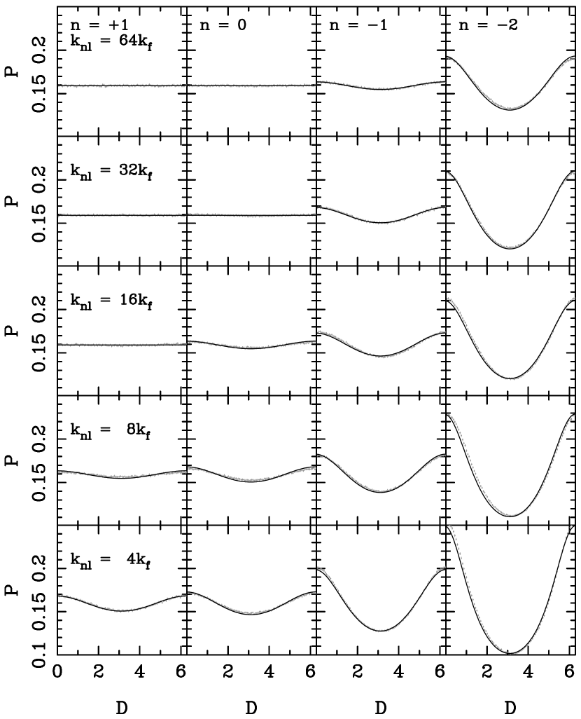
Figure 1: Histograms $P(D)$ of phase differences $D$ are shown in grey along with the analytical model (8) for four different initial spectra as functions of epoch. Close agreement makes it difficult to discriminate between data and theory.

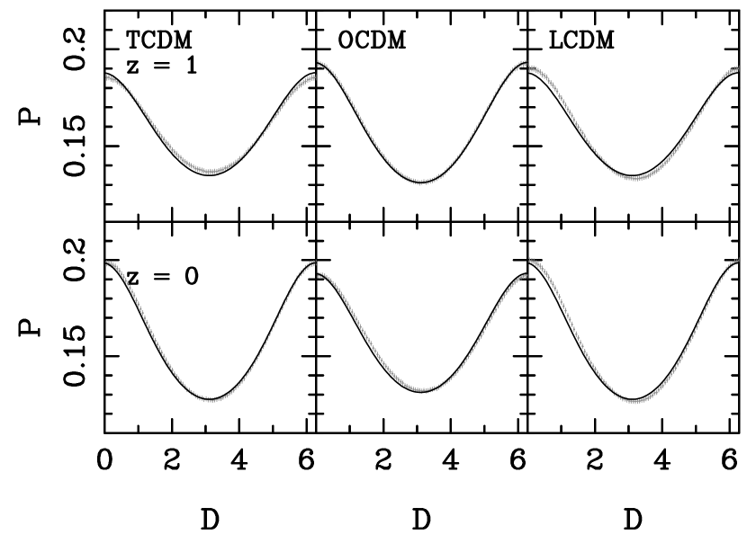
Figure 2: Histograms $P(D)$ of phase differences $D$ are shown in grey along with the analytical model (8) for three different CDM models as functions of epoch.

References

- Albrecht & Steinhardt (1982) Albrecht, A., and Steinhardt, P. J. 1982, Phys. Rev. Lett., 48, 1220
- Bardeen et al. (1986) Bardeen, J. M., Bond, J. R., Kaiser, N., and Szalay, A. S. 1986, ApJ, 304, 15
- Chiang (2001) Chiang, L.-Y. 2001, MNRAS, 325 405
- Chiang & Coles (2000) Chiang, L.-Y., and Coles, P. 2000, MNRAS, 311, 809
- Chiang, Coles, & Naselsky (2002) Chiang, L.-Y., Coles, P., and Naselsky, P. D. 2002, MNRAS, 337, 488
- Coles & Chiang (2000) Coles, P., and Chiang, L.-Y. 2000, Nature, 406, 376
- Fan & Bardeen (1995) Fan, Z., and Bardeen, J. M. 1995, Phys. Rev. D., 51, 6714
- Fisher (1993) Fisher, N. I. 1993, Statistical Analysis of Circular Data (Cambridge: Cambridge University Press)
- Guth (1981) Guth, A. H. 1981, Phys. Rev. D., 23, 347
- Guth & Pi (1982) Guth, A. H. and Pi, S.-Y. 1982, Phys. Rev. Lett., 49, 1110
- Jain & Bertschinger (1998) Jain, B., and Bertschinger, E. 1998, ApJ, 509, 517
- Linde (1982) Linde, A. 1982, Phys. Lett. , B108, 389
- Mardia (1972) Mardia, K. V. 1972, Statistics of Directional Data (London: Academic Press)
- (14) Melott, A. L., Coles, P., Feldman, H. A., and Wilhite, B. 1998, ApJ, 496, L85
- Melott & Shandarin (1993) Melott, A. L., and Shandarin, S. F. 1993, ApJ, 410, 469
- Ryden & Gramann (1991) Ryden, B. S., and Gramann, M. 1991, ApJ, 383, L33
- Scherrer, Melott & Shandarin (1991) Scherrer, R. J., Melott, A. L., and Shandarin, S. F. 1991, ApJ, 377, 29
- Scoccimarro, Couchman & Frieman (1999) Scoccimarro, R., Couchman, H. M. P., and Frieman, J. A. 1999, ApJ, 517, 531
- Soccimarro, Zaldarriaga & Hui (1999) Scoccimarro, R., Zaldarriaga, M., and Hui, L. 1999, ApJ, 527, 1
- Soda & Suto (1992) Soda, J., and Suto, Y. 1992, ApJ, 396, 379
- Verde et al. (2001) Verde, L., Jimenez, R., Kamionkowski, M., and Matarrese, S. 2001, MNRAS, 325, 412
- Verde et al. (2000) Verde, L., Wang, L., Heavens, A. F., and Kamionkowski, M. 2000, MNRAS, 313, 141
- Watts & Coles (2003) Watts, P. I. R., and Coles, P. 2003, MNRAS, 338, 806