The Soft X-ray Spectrum from NGC 1068 Observed with LETGS on Chandra

Using the combined spectral and spatial resolving power of the Low Energy Transmission Grating (LETGS) on board Chandra, we obtain separate spectra from the bright central source of NGC 1068 (Primary region), and from a fainter bright spot 4″ to the NE (Secondary region). Both spectra are dominated by discrete line emission from H- and He-like ions of C through S, and from Fe L-shell ions, but also include narrow radiative recombination continua (RRC), indicating that most of the observed soft X-ray emission arises in low-temperature ($kT_{\mathrm{e}}\sim$ few eV) photoionized plasma. We confirm the conclusions of Kinkhabwala et al. (2002b ), based on XMM-Newton Reflection Grating Spectrometer (RGS) observations, that the entire nuclear spectrum can be explained by recombination/radiative cascade following photoionization, and radiative decay following photoexcitation, with no evidence for the presence of hot, collisionally ionized plasma. In addition, we show that this same model also provides an excellent fit to the spectrum of the Secondary region, albeit with radial column densities roughly a factor of three lower, as would be expected given its distance from the source of the ionizing continuum. The remarkable overlap and kinematical agreement of the optical and X-ray line emission, coupled with the need for a distribution of ionization parameter to explain the X-ray spectra, collectively imply the presence of a distribution of densities (over a few orders of magnitude) at each radius in the ionization cone. Relative abundances of all elements are consistent with Solar abundance, except for N, which is 2–3 times Solar. Finally, the long wavelength spectrum beyond 30 Å is rich of L-shell transitions of Mg, Si, S, and Ar, and M-shell transitions of Fe. The velocity dispersion decreases with increasing ionization parameter, which has been deduced from the measured line intensities of particularly these long wavelength lines in conjunction with the Fe-L shell lines.

1 Introduction

The bright Seyfert 2 galaxy, NGC~1068, has been studied extensively for many years at optical, UV, IR, radio, and X-ray wavelengths. In the unified model of active galactic nuclei (AGN) (Miller & Antonucci miller (1983); Antonucci & Miller antonucci85 (1985); Antonucci antonucci93 (1993)), the soft X-ray spectra of Seyfert 2 galaxies are expected to be strongly affected by emission and scattering in a medium irradiated by the nuclear continuum. However, soft X-ray emission can also be produced by collisionally-heated gas associated with shocks in starburst regions (Wilson et al. wilson (1992)). High resolution X-ray spectroscopy, now becoming available with the grating spectrometers on Chandra and XMM-Newton, can provide a means of distinguishing between these two interpretations.

Recently, Kinkhabwala et al. (2002b ) presented the X-ray spectrum of the nuclear regions in NGC 1068 obtained with the Reflection Grating Spectrometer (RGS) on XMM-Newton. They show that the soft X-ray emission is dominated by lines from H-like and He-like ions of all low-Z elements from C through Si, as well as a complex of L-shell lines from Ne-like through Li-like Fe. Most of the lines are significantly blueshifted and broadened, with characteristic velocities $\sim$ several hundred km s^-1. Of particular interest is the presence of strong and narrow RRC of C, N, O, and Ne ions, which imply that most of the observed soft X-ray flux arises in low-temperature ($kT\sim$ few eV) plasma. There is also excess emission (relative to pure recombination) in all higher series resonance lines of the H-like and He-like species, which is shown to be a result of direct photoexcitation by the continuum.

Kinkhabwala et al. (2002b ) further present a new quantitative model for the nuclear regions of NGC 1068 that provides an excellent fit to their observed spectrum. The model involves a cone of warm plasma photoionized and photoexcited by the same nuclear power-law continuum (Kinkhabwala et al. 2002a ). In this model, each ionic line series is fit independently, with only three free parameters: the radial column density for that ion, the velocity width, and the overall normalization (the product of the nuclear luminosity and the covering factor). Interestingly, the derived column densities are consistent with those measured using absorption features in high resolution X-ray spectra of Seyfert 1 galaxies, thereby providing strong support for the unified model.

Given the 15″ spatial resolution of the XMM-Newton telescopes, it was not possible with the RGS data to derive any useful information on the spatial dependence of the observed emission line spectrum. This issue is best addressed with the transmission grating spectrometers on the Chandra X-ray Observatory. In this paper, we present the data acquired with the LETGS (see also the companion paper presenting HETGS data by Ogle et al. ogle (2002)). Earlier Chandra imaging observations of NGC 1068 (Young et al. young (2001)) had shown the presence of a bright compact source, $\sim$ 1″.5 or $108$ pc in extent (1″= $72$ pc), taking the distance to NGC 1068 to be 14.4 Mpc (Bland-Hawthorn et al. bland-hawthorn (1997)). This is coincident with the brightest radio and optical emission, together with an extended cone of emission (out to 7″; 504 pc) pointing to the NE, which coincides with the NE radio lobe and gas in the narrow line region. A discrete region of emission is observed in the cone at about 4″ ($288$ pc) from the bright compact source. We show here that the spectrum of this region differs significantly from that of the compact central source, but that it is also well described by the same radiation-driven model presented by Kinkhabwala et al. (2002b ), albeit with lower radial column densities. The lower column densities are expected, and are a natural consequence of the larger distance of this extended gas from the source of the ionizing continuum.

The LETGS also has a significantly larger bandpass than the RGS and allows us to investigate the nature of the spectrum down to the region of the Fe K-shell transitions near $2$ Å, and out beyond $35$ Å, where we detect L-shell transitions of Ar, S, Si, and Mg.

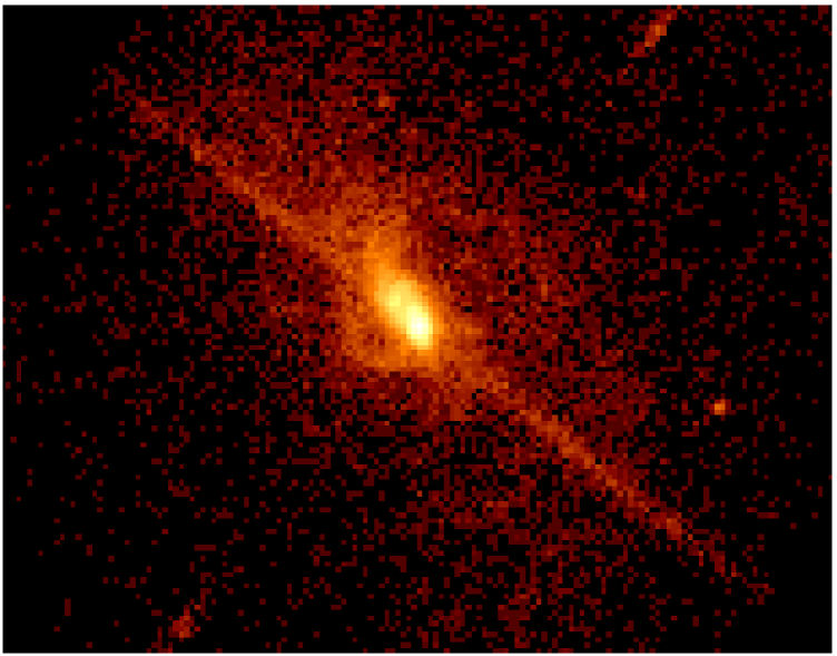
Figure 1: LETGS zero order image. North is up and East is left. The strong bar (top left-bottom right) represents ”out of time events” from the CCD-readout. The beginning of the spectral image, minus order bottom left and positive orders, top right can just be seen. Notice the dispersion direction is close to perpendicular to the extended NE-direction. The point source in the lower right quadrant has a very hard spectrum. The angular size of the total image is 60″$\times$ 75″.

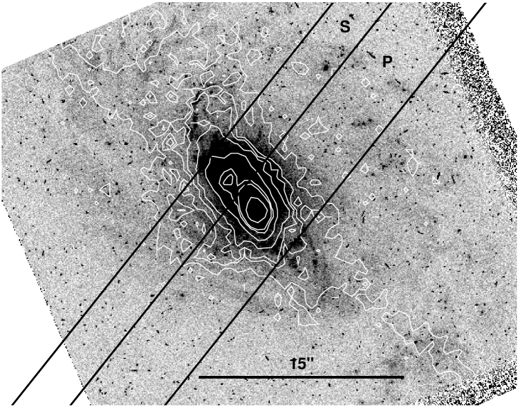
Figure 2: Zero-order X-ray intensity contours plotted over an optical [O iii] (5007 Å) HST image (Bruhweiler et al. bru (2001)). The Primary (“P”) and Secondary (“S”) extraction regions are indicated. The X-ray/optical correlation is remarkably good.

2 Observation and Data Analysis

Since the extended nature and the orientation of the X-ray emission from NGC 1068 were known prior to the time the grating observations were planned, the roll angle was selected such that the dispersion angle was nearly perpendicular to the NE extent, making it possible to separately study the emission from the central nuclear component (hereafter, the Primary region), and a bright spot in the extended ionized cone (hereafter, the Secondary region). The HETGS (Ogle et al. ogle (2002)), and the LETGS (this work) observed the source on December 4 and 5, 2000, for 46 ks and 77 ks, respectively. The LETGS configuration for this measurement involved the ACIS-S as the readout detector, in place of the usual HRC. We used CIAO version 2.1 to generate the event file. In order to verify the wavelength scale as generated with CIAO, we ran a Capella calibration observation (OBSID 00055), and did a recursion analysis based on a few strong spectral lines. There appears to be a very small systematic offset proportional to the wavelength, which is close to a similar systematic offset found during the analysis of the HETGS measurement of NGC 4151 (Ogle et al. ogle2000 (2000)). The correction is $+0.7$ mÅ per Å.

The LETGS zero order image is displayed in Fig. 1. The diagonal streak in this image is not the dispersed spectrum, it arises from “out of time” events in the CCD-readout. The short wavelength edges of the spectrum can be discerned as spots in the lower left and upper right of the figure. Note that the source extent is nearly perpendicular to the dispersion direction. In Fig. 2, this X-ray image is shown as a contour plot overlayed on an [O iii] optical image obtained by HST. As can be seen, the X-ray extension correlates well with the extended [O iii] emission. We have indicated in Fig. 2 the source extraction regions, which we use to isolate the spectrum of the Primary and Secondary regions.

A spatial cut through this zero order image in the cross-dispersion direction is plotted in Fig. 3. Clearly visible on the left side (NE-direction) is the small Secondary peak, which corresponds to our Secondary region. Here again, the extraction regions for the Primary and Secondary spectra are indicated. The boundary between them was chosen based on the O vii line ratio variation along the cross-dispersion direction (see Sect. 3).

The zero order profile in the dispersion direction of the Primary region is well represented by a Gaussian with the centroid at $-0.0056\pm 0.0007$ Å, and with a width given by $\sigma=0.0317\pm 0.0008$ Å. This profile is slightly broader than the instrument profile for a point source ($\mathrm{FWHM}=0.06$ Å; $\sigma=0.0255$ Å), and is therefore affected by the geometry of the source extent. Similarly, the profile of the Secondary region in the dispersion direction is represented by a Gaussian, with the centroid at $+0.032\pm 0.002$ Å, and with a width $\sigma=0.062\pm 0.002$ Å.

We checked for time variability in the zero order flux. As is to be expected for this spatially extended source, we find no significant variations on timescales in the range $\sim$ few seconds up to the length of the observation.

Figure 3: Intensity as a function of the cross dispersion direction. The Primary (“P”) and Secondary (“S”) regions are indicated.

Figure 4: Spectrum of the Primary region between 1.5 and $60$ Å, in five panels to cover the full range. The bin size is equal to $0.025$ Å.  Indicated are some of the strongest lines. All panels are the positive and negative orders taken together.

Figure 5: Spectrum of the Secondary region, wavelength scales as in previous figure for easy comparison.

3 Spectral Analysis

We present spectra of the Primary and Secondary regions in Figs. 4 and 5, respectively. We combine $m=-1$ and $m=+1$ orders to obtain these spectra. Both spectra are plotted over the full range of the LETGS of $\sim 1.5-60$ Å.

The Primary region contains approximately ninety percent of the flux (”P” region in Figs. 2 and 3). As is expected, this spectrum closely resembles the RGS spectrum (Kinkhabwala et al. 2002b ), which contains all of the soft-X-ray flux from NGC 1068. In addition to the H-like and He-like series of C, N, O, Ne, Mg, and Si and Fe L-shell transitions (from Fe xvii–Fe xxiv), which were observed by the RGS, the LETGS also extends down to Fe K at $1.8$ Å, and, at longer wavelengths, from the He-like C triplet at $40-42$ Å (which is just outside the RGS range) out to $60$ Å, resolving a forest of lines from L-shell transitions in mid-Z ions such as Ar, S, Si, and Mg. We also note that lines in the $\sim 5-10$ Å region of the specrum, though detected by the RGS, are better resolved by the LETGS.

As was also found in the RGS spectrum, the LETGS resolves several prominent RRC, which, in addition to the relative strength of the forbidden line in the He-like triplets, provides the main evidence for recombination in low temperature, photoionized plasma. Many higher order transition lines, observed by the RGS, are also resolved by the LETGS; these lines are indicative of photoexcitation (e. g., Sako et al. sako (2000)).

Overall, many features observed in the Primary spectrum are also observed in the spectrum of the Secondary region (”S” region in Figs. 2 and 3), which comprises approximately ten percent of the total flux from NGC 1068.

Table 1: He-like $R$ ratios for Primary and Secondary region spectra.

Ion	Primary	Secondary
C v	$11\pm 17$	$1.5\pm 1.1$
N vi	$3.3\pm 1.5$	—
O vii	$5.4\pm 0.9$	$4.5\pm 2.0$
Ne ix	$2.3\pm 0.5$	$1.4\pm 0.6$

Table 2: He-like $G$ ratios for Primary and Secondary region spectra.

Ion	Primary	Secondary
C v	$2.5\pm 1.4$	$1.8\pm 1.3$
N vi	$3.0\pm 1.1$	$1.1\pm 0.9$
O vii	$4.6\pm 0.9$	$1.6\pm 0.4$
Ne ix	$2.0\pm 0.3$	$1.4\pm 0.4$

One main difference between the two spectra is in the He-like triplet ratios, $R=f/i$ and $G=(i+f)/r$, which are listed for several He-like ions in the Primary and Secondary spectra in Tables 1 and 2.

The $G$ ratios in the Primary spectrum are inconsistent with either pure recombination or collisional ionization equilibrium, suggesting the presence of photoexcitation, as was concluded for the RGS spectrum (Kinkhabwala et al. 2002b ). The $G$ ratios in the Secondary region are consistent with hot collisional plasma or with photoexcitation in a recombining, photoionized plasma.

The $R$ ratios are overall less useful for distinguishing between pure recombination and collisional ionization equilibrium. They are also more difficult to measure due to the weakness and/or blending of the intercombination line in most triplets. However, we note that the well-measured $R$ ratio for O vii is significantly greater than expected for pure recombination, as was also found in Kinkhabwala et al. (2002b ), who suggested that this may be due to inner-shell ionization of O vi (e.g., Kinkhabwala et al. 2002a ).

Figure 6: Forbidden line to resonance line ratio of the O vii triplet as a function of cross dispersion angle. The bins along the cross dispersion axis are one arcsec wide; negative numbers are in the NE direction, positive numbers in the SW direction and bin zero is centered at the maximum intensity. One clearly notices an abrupt change over from a value of 3.6$\pm$0.6 for the Primary region to 1.0$\pm$0.3 for the Secondary region, around the boundary between these regions at $-$2″.

Since the O vii triplet is the strongest feature in both spectra and since the line ratios are different for both spectra, we measured the forbidden-to-resonance line ratio $f/r$ as a function of cross-dispersion, in steps of 1″, see Fig. 6. There are clearly two distinct regimes, the Primary region with a high ratio of $f/r=3.6\pm 0.6$, and the Secondary region with a value of $1.0\pm 0.3$. This changeover occurs within a spatial extent of less than one arcsec.

3.1 Fits Using an Irradiated Cone Model

We find that the H-like and He-like ionic line series observed in the Primary and Secondary region spectra are fit well with a simple irradiated cone model, as was used for the RGS spectrum of NGC 1068 (Kinkhabwala et al. 2002b ). The cone is irradiated at its tip by an inferred nuclear power-law continuum. Though our view to the nucleus is completely obscured by intervening material (dusty torus), our perpendicular view of the irradiated cone is unobscured, allowing for observation of recombination/radiative cascade following photoionization, and radiative decay following photoexcitation. This simple irradiated cone model has been incorporated into XSPEC as the local model photo (Kinkhabwala et al. 2002a ), which has been used to generate the fits to the Primary and Secondary regions as presented below.

We assume that the overall normalization, $fL_{X}$, which is the covering factor $f=\Omega/4\pi$ times the power-law luminosity $L_{X}$ is the same for all ions. For ease of comparison of the LETGS results with the RGS results and between the Primary and Secondary region spectra, we assume the same value for the normalization of $fL_{X}=10^{43}$ ergs s^-1.

We also assume a single radial velocity distribution specified by Gaussian width $\sigma_{v}^{\mathrm{rad}}$. The velocity width needed to explain the Primary region spectrum of $\sigma_{v}^{\mathrm{rad}}=100$ km s^-1, however, is a factor of two smaller than that required to explain the RGS spectra. For simplicity, we use this velocity width for the Secondary region as well.

The only free parameters left are the individual radial ionic column densities. We allow for individual line absorption, but assume that photoelectric absorption is negligible. With this assumption, we can simplify the calculations by irradiating each ionic column density separately with an initially unabsorbed power law, since the effect of individual line absorption due to all other ions, which removes only a small fraction of the flux, can be safely neglected. Alternatively, using the method employed by photo, we can irradiate all ionic column densities together, assuming all ions have the same radial distribution. The radial ionic column densities we infer below are indeed consistent with the assumption of negligible photoelectric absorption, and we have checked that either method yields the same result. Moreover, as we argue in Sect. 6, there likely exists a broad range of densities at each radius, implying that the assumption that all ions have a similar radial distribution may also be physically correct.

We demonstrate below that these simple model assumptions allow for a good fit to both the Primary and Secondary region spectra.

3.1.1 Primary Region

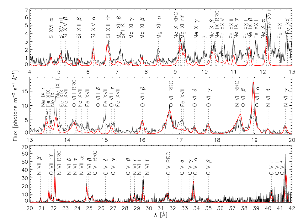
Figure 7: Fluxed spectrum of the first order of the Primary region, together with the model. The model does not yet include Fe L-shell transitions.

Using the above-quoted global values of $fL_{X}=10^{43}$ ergs s^-1 and $\sigma_{v}^{\mathrm{rad}}=100$ km s^-1, we have fit the individual radial ionic column densities. The best fit values are given in Table 3, and the final fit using these values is shown in Fig. 7. These column densities are very similar to the results obtained for the RGS spectrum.

The ratio of the ground state RRC to the 2p$\rightarrow$1s transitions for each ion rules out the presence of any additional hot, collisional plasma. The forbidden lines in the He-like triplets of N, O, and Ne, however, appear significantly stronger than predicted. This is likely due to inner shell ionizations in the corresponding Li-like ions, which enhance only the forbidden line in the triplet (for further explanation, see, e. g., Kinkhabwala et al. 2002a ). This observation and proposed mechanism was also noted in the RGS paper (Kinkhabwala et al. 2002b ).

3.1.2 Secondary Region

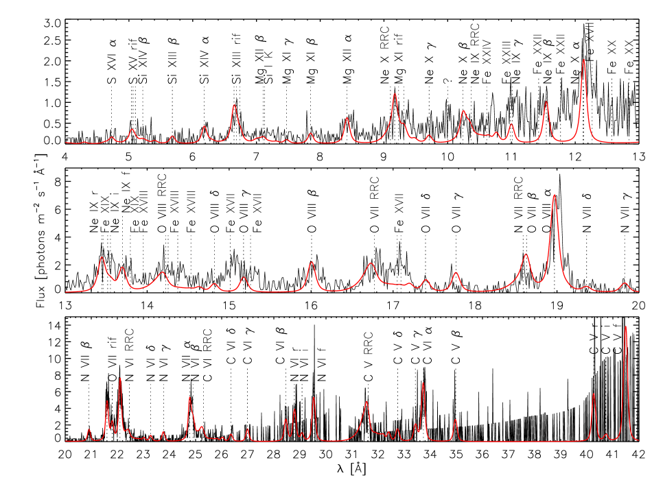
Figure 8: Spectrum of the Secondary region, together with the model.

Using the same global values as above, we have fit the column densities for the Secondary region. The best fit values are given in Table 3, and the final fit is shown in Fig. 8. The column densities for the Secondary region are a factor of a few less than the column densities inferred for the Primary region.

The explanation for this enhancement of the resonance line for lower column density is simple (Kinkhabwala et al. 2002b ). Keeping $\sigma_{v}^{\mathrm{rad}}$ constant, at low column densities the resonance line is dominant in the He-like triplet, since this transition has a high oscillator strength and is unsaturated. At higher column densities this transition begins to saturate, and recombination begins to increase in significance (since the photoelectric edge saturates only at high column density). Generically, then, at low column densities, the resonance line is relatively strong, but at high column densities, it saturates, becoming relatively weaker compared to lines due to pure recombination.

The ratio of the RRC to the 2p$\rightarrow$1s transitions again rules out the presence of a significant additional hot, collisional plasma. Though, given the lower quality of the Secondary spectrum compared to the Primary spectrum, this conclusion is correspondingly less robust. However, the presence of strong higher order lines (np$\rightarrow$1s), such as N vii Ly$\gamma$ and O vii He$\delta$, which can only be explained by photoexcitation, strengthens the argument against an additional hot, collisional plasma contribution (Kinkhabwala et al. 2002b ). The formal upper limit to the emission measure of any hot, collisional plasma in the 0.2–1 keV temperature range is $10^{62}$ cm^-3 for the Secondary region and $2\times 10^{62}$ cm^-3 for the Primary region.

We also note that the temperatures for the RRC are the same as for the Primary region (in particular, compare the RRC of O vii in both spectra).

Table 3: NGC 1068 Ionic column densities of Primary and Secondary regions. Italicized values for the temperatures were taken arbitrarily for ions which do not show clear RRC.

Ion	Nion Primary	Nion Secondary	$kT$ (eV)
C v	7.$10^{17}$	3.$10^{17}$	2.5
C vi	8.$10^{17}$	4.$10^{17}$	4
N vi	3.$10^{17}$	1.$10^{17}$	3
N vii	5.$10^{17}$	1.$10^{17}$	4
O vii	7.$10^{17}$	2.$10^{17}$	4
O viii	6.$10^{17}$	2.5.$10^{17}$	6
Ne ix	2.$10^{17}$	8.$10^{16}$	10
Ne x	1.$10^{17}$	6.$10^{16}$	10
Mg xi	1.$10^{17}$	2.5.$10^{16}$	10
Mg xii	1.$10^{17}$	2.$10^{16}$	10
Si xiii	1.1.$10^{17}$	3.$10^{16}$	10
Si xiv	1.1.$10^{17}$	2.$10^{16}$	10
S xv	4.$10^{16}$	1.$10^{16}$	10
S xvi	6.$10^{16}$	1.$10^{16}$	10

3.2 Elemental Abundance Estimates

In order to obtain an estimate of the relative elemental abundances, we derive a total hydrogen column density from the individual ionic column densities assuming Solar abundances. This hydrogen column density $N_{\rm H}$ is a function of the ionization parameter ($\xi$), according to the $\xi$ in which each ion forms. For this analysis, we employ the same set of photoionization balance calculations from XSTAR (Kallman & Krolik Kallman & Krolik (1995)) as used in the analysis of the Seyfert 1 galaxy NGC 5548 (Kaastra et al. kaastra2002 (2002)) and assume that the observed flux for each ion originates predominantly from plasma at an ionization parameter where the relative concentration of that ion reaches a maximum. Adopting Solar abundances from Anders & Grevesse (anders (1989)), except for the recently improved measurement of the Solar O abundance taken from Allende Prieto et al. (allende (2001)), we obtain $N_{\rm H}(\xi)$ for the Primary component as plotted in Fig. 9.

Note that these column densities are consistent with the estimated column of log $N_{\rm H}$ = $\sim$21.9 derived from the L-shell lines (Sect. 5). As explained in detail in that section, this value of $N_{\rm H}$ is consistent with the observed line fluxes measured for the Fe lines assuming that they arise exclusively from photoexcitation. However, since most of the bright Fe lines are saturated, this estimate is very uncertain and thus of less value for abundance measurements. We estimate the accuracy of the column densities based on the K-shell lines to be within $\sim$ 25 % (relative to each other). The error bars in Fig. 9 reflect these

Figure 9: Derived hydrogen column density as a function of ionization parameter for C, N, O, Ne, Mg, Si and S.

The data point corresponding to H-like Ne in Fig. 9 seems to be somewhat low compared with the general trend suggested by the other ions. Therefore we consider this point on the plot less trustworthy for an abundance analysis. This inconsistency could be due to the Ly$\alpha$ line of Ne x being contaminated by Fe xvii.

Deviations from Solar abundances in Fig. 9 would appear as clear vertical offsets between elements that cover similar regions of $\xi$. However, it can be seen that obvious offsets between elements are not seen. In fact, the column density $N_{\rm H}$ does not vary by much in the observable range of $\xi$. This implies that for the most part the relative abundances (no measurement is available for H) are consistent with Solar, or at least that there are no conclusive deviations, of more than about $\pm$50%, from Solar abundances. On the face of it, this is in stark contrast with previous moderate-resolution X-ray observations of NGC 1068 as well as with UV and optical measurements from the narrow line region. Netzer & Turner (netzer (1997)) as well as Marshall et al. (marshall (1993)) have fitted the ASCA and BBXRT X-ray spectra, respectively, of NGC 1068 with models that require an Fe/O abundance ratio of more than 8 times Solar. This could be attributed to the severely incomplete Fe-L model that was used in those works. Also, photoexcitation was not treated explicitly as shown to be necessary in Kinkhabwala et al. (2002b ). In the ASCA case, the weak signal in the low-energy region of the O features might also be to blame. On the other hand, the result of those papers that all other abundances except for Fe and O are Solar is consistent with the present measurement, with the exception of N as discussed below. Nitrogen apparently was not included in those earlier models.

According to Fig. 9, N is the only element that seems to lie consistently above the data points of other elements (namely O and C) with which it overlaps in $\xi$ space. The N abundance enhancement found here is of the order of a factor 2$-$3 compared to C and O (also observed in Kinkhabwala et al. 2002b ). This could be due to an enrichment of the AGN medium by WR type stars close to the nucleus. An enrichment of nitrogen has also been found in other AGN, for example in IRAS 13349+2438 (Sako et al. sako2001 (2001)). Finally, we note that for the Secondary region, we find very similar results only that the $N_{\rm H}$ is about $10^{21}$ cm^-2, which is 3$-$5 times smaller than for the Primary region. Additionally, the error bars for the Secondary region are obviously larger than for the Primary region.

4 Line Broadening and Line Shifts

4.1 Line Broadening

Table 4: Line strengths and velocity shifts of some of the stronger lines in the Primary and Secondary region. Line strengths are at the source and in units of $10^{48}$ photons s^-1. We adopt a galactic absorption $N_{\mathrm{H}}=2.95\times 10^{20}$ cm^-2 (Murphy et al. mur (1996)) and a redshift of $z=0.00379\pm 0.00001$ (Huchra et al. huchra (1999)). The errors quoted are statistical errors; the systematic error in the velocities in columns 5 and 6 range from 100 to 30 km s^-1 for Si and O, respectively. All velocity values are quoted with respect to the systemic velocity. The line strengths and $\Delta v$ values of the Ne x Ly$\alpha$ line are probably contaminated with Fe-L lines and are therefore considered less reliable.

Line ID	Pred. $\lambda$	Primary	Secondary	$\Delta$vPrimary	$\Delta$vSecondary
	Å	photons (1048s-1)	photons (1048s-1)	km s-1	km s-1
Si xiv Ly$\alpha$	6.180	0.22$\pm$0.03	0.05$\pm$0.02	$-$ 940$\pm$290	+ 470 $\pm$1650
Mg xii Ly$\alpha$	8.419	0.25$\pm$0.03	0.12$\pm$0.03	$-$ 1000$\pm$360	+ 290 $\pm$1030
Ne x Ly$\alpha$	12.132	0.83$\pm$0.11	0.50$\pm$0.08	$-$ 550$\pm$150	+ 1450 $\pm$590
O viii Ly$\alpha$	18.969	2.95$\pm$0.27	1.40$\pm$0.18	$-$ 470$\pm$100	+ 430$\pm$190
O vii f	22.101	8.96$\pm$0.55	1.29$\pm$0.24	$-$ 250$\pm$20	+ 360$\pm$160
N vii Ly$\alpha$	24.779	3.69$\pm$0.94	0.80$\pm$0.16	+ 15$\pm$360
C vi Ly$\alpha$	33.734	4.69$\pm$0.68	1.21$\pm$0.31	$-$ 300$\pm$120	$-$ 860$\pm$330
C v f	41.472	6.44$\pm$1.99	1.01$\pm$0.40	$-$ 380$\pm$160

We have used a number of strong emission lines, the Ly$\alpha$ lines of Si, Al, Mg, Ne, O, N and C, and the forbidden lines of the He-like triplets of O and N, to look for velocity broadening (Table 4. All lines of the Primary region appear to be broader than the zero order profile, although the formal errors are large. The most reliable velocity numbers are obtained from ${O\textsc{viii}}$ Ly $\alpha$ and the forbidden line of the ${O\textsc{vii}}$ triplet, $\sigma_{v}$ being 600 and 320 km/s, respectively. The Si, Al, and Mg Ly$\alpha$ lines show values of about 1000 km/s but with large errors. Fig. 10 shows the O vii forbidden line of the Primary region in velocity space.

For the Secondary region the measured widths of the lines are consistent with zero, with upper limits of about 1000 km s^-1.

Figure 10: Spectrum of the O vii forbidden line in $+1$ order for the Primary region. The velocity scale is set with respect to the rest frame of NGC 1068. The solid line shows the best fit model with an average blueshift of $-250$ km/s and a velocity broadening of $320$ km/s. The dashed line is the best fit with no velocity shift and broadening. Note that in the latter case the line profile is given by the zeroth order profile of the Primary as discussed in Sect. 3.1. The bin size in wavelength space is $25$ mÅ.

Figure 11: Spectrum of the O vii forbidden line in $+1$ order for the Secondary region. The velocity scale is set with respect to the rest frame of NGC 1068. The solid line shows the best fit model with an average redshift of $+360$ km/s and no velocity broadening. The dashed line is the best fit with no velocity shift and broadening. Note that in the latter case the line profile is given by the zeroth order profile of the Secondary as discussed in Sect. 3.1. The bin size in wavelength space is $37.5$ mÅ.

4.2 Line Shifts

We used the same set of lines to look for redshifts or blueshifts. First of all we find for most lines of the central region a difference between the measured positive and negative spectral order position of about $0.02$ Å. One would however expect a difference of $\sim 0.01$ Å, based on the difference between the peak position of the Gaussian fit to the zero order distribution and the zero point of the wavelength scale. The underlying assumption is that the line radiation distribution coincides with the total zero order radiation distribution. We verified the line wavelength obtained above by fitting the measured line shape to a Gaussian and forced the line width to be equal to the zero order width; that has very little effect on the line wavelength determination. The results of fitting the positive and negative spectral order lines together, are summarized in Table 4. We then looked for possible differences in redshift or blueshift between the Secondary and Primary region.

Fitting for the Secondary region, the positive and negative spectral orders together lead to redshifts, also listed in Table 4. (All shifts are calculated with respect to the systemic velocity).

5 Long Wavelength L-shell Line Detections

We have also analysed the long wavelength part of the LETGS spectrum of the Primary component (beyond 30 Å). This part of the spectrum contains the L-shell complexes of Ne, Mg, Si, S, Ar and Ca. We have determined the fluxes of the strongest resonance lines in the $15-60$ Å band (see Table 5). Wavelengths and oscillator strengths for these lines are the same as those quoted in Kaastra et al. (kaastra2002 (2002)). The data are taken from what is used in their slab and xabs models, and for the relevant ions they are derived mostly from the compilation by Verner et al. (verner96 (1996)); updates in some cases, using calculations with HULLAC (Bar-Shalom et al. bar-s (2001)), were provided by Liedahl (see Kaastra et al. kaastra2002 (2002) for more details). In addition, we have included a number of Fe-L transitions in the table. For some ions we did not use the strongest line. An example is Fe xix, where the strongest lines are blended by lines from Ne ix. Finally, in a few cases we co-added lines from the same ion if they could not be resolved with the LETGS.

Table 5: Wavelengths, oscillator strength, ionization parameters and line fluxes for the strongest lines of each species in the Primary component. Line strengths are given in units of $10^{48}$ ph/s.

Ion $\lambda$ $f$ $\log\xi$ Flux Flux (Å) observed model Ne viii 57.75 0.01 1.0 2.7$\pm$ 4.2 2.2 Mg ix 48.34 0.14 1.2 3.6$\pm$ 1.3 3.1 Mg x 57.88 0.22 1.5 6.0$\pm$ 5.0 4.7 Si viii 50.02 0.12 0.6 2.9$\pm$ 1.4 2.9 Si ix 55.30 0.95 0.9 5.9$\pm$ 3.0 4.5 Si x 50.52 0.60 1.3 4.3$\pm$ 1.7 5.1 Si xi 43.76 0.48 1.7 4.7$\pm$ 1.0 3.2 Si xii 40.91 0.23 2.0 3.0$\pm$ 5.1 2.2 S vii 51.81 0.61 0.0 3.4$\pm$ 1.8 3.9 S viii 52.77 0.89 0.4 3.7$\pm$ 2.3 4.1 S ix 47.43 0.38 0.8 2.7$\pm$ 1.0 3.2 S x 42.54 0.67 1.1 4.0$\pm$ 4.3 3.3 S xi 39.24 1.05 1.4 3.3$\pm$ 2.2 4.1 S xii 36.40 0.62 1.7 3.1$\pm$ 1.3 2.5 S xiii 32.24 0.45 2.0 2.5$\pm$ 0.8 2.1 S xiv 30.44 0.34 2.4 1.6$\pm$ 1.0 0.6 Ar x 37.43 0.65 1.0 3.6$\pm$ 1.7 1.4 Ar xi 34.33 0.42 1.3 2.9$\pm$ 1.0 1.0 Ar xii 31.39 0.87 1.5 4.2$\pm$ 0.9 1.5 Ar xiii 29.32 0.91 1.8 1.7$\pm$ 0.7 1.2 Ar xiv 27.47 0.65 2.1 0.7$\pm$ 0.5 0.8 Ca xi 30.45 2.34 1.2 1.6$\pm$ 1.0 1.5 Ca xii 27.97 1.30 1.3 0.2$\pm$ 0.4 1.0 Ca xiii 25.53 0.47 1.6 0.3$\pm$ 0.2 0.4 Ca xiv 24.13 0.89 1.9 0.4$\pm$ 0.2 0.6 Ca xv 22.73 0.93 2.1 0.5$\pm$ 0.2 0.4 Ca xvi 21.45 0.66 2.4 0.9$\pm$ 0.5 0.2 Ca xvii 19.56 0.65 2.5 0.2$\pm$ 0.1 0.2 Ca xviii 18.70 0.37 2.8 0.3$\pm$ 0.3 0.1 Fe xiv 58.96 0.28 1.4 5.4$\pm$ 8.5 4.5 Fe xv 52.91 0.41 1.6 4.3$\pm$ 2.5 4.7 Fe xvi 50.35 0.16 1.6 5.4$\pm$ 1.9 2.4 Fe xvii 15.01 2.72 2.1 1.6$\pm$ 0.3 1.6 Fe xviii 14.20 0.88 2.3 0.8$\pm$ 0.2 1.2 Fe xix 13.80 0.21 2.5 0.4$\pm$ 0.2 0.3 Fe xx 12.84 0.93 2.8 0.7$\pm$ 0.2 0.4 Fe xxi 12.29 1.24 3.0 0.3$\pm$ 0.1 0.4 Fe xxii 11.71 0.67 3.1 0.2$\pm$ 0.2 0.3 Fe xxiii 8.30 0.14 3.3 0.1$\pm$ 0.1 0.1 Fe xxiv 10.64 0.37 3.4 0.2$\pm$ 0.2 0.2

Given the limited and not homogeneously tested accuracy of the wavelengths, and also the possibility of some blending we cannot always be sure of the derived fluxes in each individual case. However, we think that the set of fluxes still reflects the overall behaviour of these ions. Not all the fluxes are statistically significant, but for the weakest lines the value given plus its nominal error bar gives at least an order of magnitude estimate of the column density of the parent ion. Table 5 lists the ionization parameter, $\xi$, for which the ion concentration reaches a maximum. We have also made model predictions for the line fluxes. We assume that for each line the emitted flux is equal to the number of photons taken away from the power law continuum ($\Gamma=1.7$, covering factor times luminosity $fL_{X}=10^{43}$ erg/s, cf. the RGS analysis of Kinkhabwala et al. 2002a ). To be more specific, we approximate the equivalent width for the absorption line by:

$$W={\lambda\sigma_{\rm v}\over c}\int\limits_{-\infty}^{\infty}[1-\exp(-\tau_{0}\mathrm{e}^{\displaystyle-y^{2}/2})]{\mathrm{d}}y,$$ (1)

with $\tau_{0}$ equal to the optical depth of the line at the line center, given by

$$\tau_{0}=0.106fN_{16}\lambda/\sigma_{\rm v,100}.$$ (2)

Here $f$ is the oscillator strength, $\lambda$ the wavelength in Å, $\sigma_{\rm v,100}$ the velocity dispersion in units of 100 km/s and $N_{16}$ the column density of the ion in units of $10^{16}$ cm^-2.

In the above, we neglected the damping wings of the lines. Equation 1 gives the equivalent width for an absorption line. The power law continuum is given by ${\mathrm{d}}N/{\mathrm{d}\lambda}=8.67\times 10^{49}\lambda^{-0.3}$ with $\lambda$ in Å. The predicted emission line flux is then simply $F=W{\mathrm{d}}N/{\mathrm{d}\lambda}$. We have divided the 40 emission lines into 4 groups of ten, each spanning a range in ionization parameter. For each group, we have determined the velocity dispersion $\sigma_{\rm v}$ and total hydrogen column density $N_{\rm H}$ that best describe the observed line fluxes (assuming Solar abundances). The results are summarized in Table 6.

Table 6: Velocity dispersion and column densities for different ranges in $\log\xi$.

$\log\xi$ $\sigma_{\rm v}$ range $\log N_{\rm H}$ range 0.0$-$1.2 170 120$-$220 21.9 lower limit 1.3$-$1.6 220 130$-$300 21.9 21.8$-$22.1 1.7$-$2.3 150 120$-$210 21.8 21.5$-$22.0 2.4$-$3.4 40 30$-$60 22.0 21.5$-$22.7

All hydrogen column densities are close to the value of $\log N_{\rm H}=21.9$, and we have adopted that value uniformly in the predicted line fluxes of Table 5. For the velocity dispersions in that table we have adopted the values of Table 6 instead. We find evidence for a significantly lower velocity dispersion at higher values of the ionization parameter. This may explain partly the problem we had with the H-like Ne and Mg lines, where we had fixed $\sigma_{\rm v}$ to $100$ km/s. The tendency of a smaller velocity dispersion for the most highly ionized material is also found in the Seyfert 1 galaxy NGC 5548, where the high ionization line of Si xiv Ly$\alpha$ is consistent with a velocity component that in the corresponding UV spectra shows up as much narrower than the lower ionized lines.

6 Summary and Conclusions

We have shown that the Chandra LETGS spectrum of the Primary region (comprising the bulk of the flux from NGC 1068) is consistent with emission from a photoionized and photoexcited cone of warm plasma, which is in accord with previous observations of this object with XMM-Newton RGS (Kinkhabwala et al. 2002b ). We have also shown, using the spatial resolution capability for angles of a few arcsec of the Chandra grating spectrometers, that the X-ray spectrum of a separate region (4$\arcsec$ to the NE), which we refer to as the Secondary, can be explained by a similar model, except with a factor of a few lower inferred radial ionic column densities. Any additional emission in either spectrum due to hot, collisional plasma is negligible.

The lower radial ionic column densities of the Secondary region as compared with the Primary region are naturally explained in the context of an irradiated cone of plasma. The radial ionic column density through each region is given in Kinkhabwala et al. (2002b ) as:

$$N^{\mathrm{rad}}_{\mathrm{ion}}\simeq 1.6\times 10^{24}A_{Z}\frac{g}{fr_{\mathrm{min,pc}}}\times$$ (3)

$$\hskip 17.07182pt\bigg{[}\frac{f_{i}}{0.5}\bigg{]}\bigg{[}\frac{(fL_{X})}{10^{43}\leavevmode\nobreak\ \mathrm{ergs\leavevmode\nobreak\ s}^{-1}}\bigg{]}\bigg{[}\frac{\xi}{1\leavevmode\nobreak\ \mathrm{ergs\leavevmode\nobreak\ cm\leavevmode\nobreak\ s}^{-1}}\bigg{]}^{-1}\leavevmode\nobreak\ \mathrm{cm}^{-2},$$

where $A_{Z}$ is the abundance relative to hydrogen, $g$ is the radial filling factor, $f=\Omega/4\pi$ is the usual covering factor, $r_{\mathrm{min,pc}}$ is the minimum radius of the cone from the nucleus in pc, and $f_{i}$ is the fractional ionic abundance. The radial dependence of $r^{-1}$ in this equation provides a simple explanation for the observed factor of a few drop in column densities in the Secondary region versus those inferred for the Primary region (Table 3), which is closer to the nucleus by at least a similar factor of a few.

An estimate of the radial filling factor of the plasma in the Secondary region is also made possible by our knowledge of $r_{\mathrm{min}}$ ($\sim$4″; $288$ pc) for this region. The inferred radial column density of $N^{\mathrm{rad}}_{\mathrm{ion}}=2.10^{17}$ for O vii in the Secondary region, along with $A_{Z}=4.89\times 10^{-4}$ and $f<0.1$, imply a radial filling factor of $g<0.07$ for plasma at the typical ionization parameter for O vii of $\xi=10$ ergs cm s^-1.

The remarkable overlap of the [O iii] and X-ray cones appears to indicate that these regions are related (Young et al. young (2001)). X-ray spectroscopy of the Primary region reveals excess blueshifts, whereas spectroscopy of the Secondary region reveals excess redshifts. These blueshifts and redshifts are comparable to the shifts observed in the same respective regions for optical/UV lines (Cecil et al. cecil1990 (1990), cecil2002 (2002); Crenshaw & Kraemer crenshaw (2000)), kinematically linking the X-ray emission regions with lower ionization state emission regions. In addition, Kraemer & Crenshaw (kraemer (2000)) argue that the optical/UV emission in the cone is also ultimately powered by photoionization due to the inferred nuclear continuum.

Using both K-shell and L-shell line series, we find that the relative abundances of all observed elements are consistent with Solar abundances, aside from N. From the relative strength of the column densities derived from K-shell emission features, we find evidence for a relative factor of 2$-$3 more N compared with C or O. Further investigation of elemental abundances is left for the future.

The K-shell transitions as well as the L-shell transitions for multiple ions, imply that a broad range in ionization parameter is present. The long wavelength emission line spectrum is very similar to what is found in Seyfert 1 galaxies in absorption. These observations provide further confirmation of the unification schemes, wherein Seyfert 1 and Seyfert 2 galaxies constitute the same objects seen from different viewing angles. The data also suggest a variation of velocity dispersion as a function of ionization parameter (see Table 6).

- (1) Allende Prieto, C., Lambert, D.L., & Asplund, M. 2001, ApJ, 556, L63
- (2) Anders, E., & Grevesse, N. 1989, Geochim. Cosmochim. Acta, 53, 197
- (3) Antonucci, R.R.J. 1993, ARA&A, 31, 473
- (4) Antonucci, R.R.J., & Miller, J.S. 1985, ApJ, 297, 621
- (5) Bar-Shalom, A., Klapisch, M., & Oreg, J. 2001, J. Quant. Spectr. Radiat. Transfer, 71, 169
- (6) Bland-Hawthorn, J., Gallimore, J.F., Tacconi, et al. 1997, Ap&SS, 248, 9
- (7) Bruhweiler, F.C., Miskey, C.L., Smith, A.M., Landsman, W., & Malumuth, E. 2001, ApJ, 546, 866
- (8) Cecil, G., Bland, J., Tully, R.B. 1990, ApJ 355, 70
- (9) Cecil, G., Dopita, M.A., Groves, B., et al. 2002, ApJ 568, 627
- (10) Crenshaw, D.M., & Kraemer, S.B. 2000, ApJ, 532, L101
- (11) Huchra, J.P., Vogeley, M.S., & Geller, M.J. 1999, ApJS, 121, 287
- (12) Kaastra, J.S., Steenbrugge, K.C., Raaasen, A.J.J., et al. 2002, A&A 386, 427
- Kallman & Krolik (1995) Kallman, T. R., & Krolik, J. H. 1995, XSTAR = A Spectral Analysis Tool, HEASARC (NASA/GSFC, Greenbelt)
- (14) Kinkhabwala, A., Behar, E., Sako, M., et al. 2002a, in preparation
- (15) Kinkhabwala, A., Sako, M., Behar, E., et al. 2002b, ApJ, accepted
- (16) Kraemer, S.B., & Crenshaw, D.M. 2000, ApJ, 544, 763
- (17) Marshall, F.E., Netzer, H., Arnaud, K.A., et al. 1993, ApJ, 405, 168
- (18) Miller, J.S., & Antonucci, R.R.J. 1983, ApJ, 271 L7
- (19) Murphy, E.M., Lockman, F.J., Laor, A., & Elvis, M. 1996, ApJS, 105, 369
- (20) Netzer, H. & Turner, T.J. 1997, ApJ, 488, 694
- (21) Ogle, P.M., Marshall, H.L., Lee, J.C., & Canizares, C.R. 2000, ApJ, 545, L81
- (22) Ogle, P.M., Marshall, H.L., Dewey, D., Lee, J.C., & Canizares, C.R. 2002, this issue
- (23) Sako, M., Kahn, S.M., Behar, E., et al. 2001, A&A, 365, L168
- (24) Sako, M., Kahn, S.M., Paerels, F., & Liedahl D.A. 2000, ApJ, 543, L115
- (25) Young, A.J., Wilson, A.S., & Shopbell, P.L. 2001, ApJ, 556, 6
- (26) Verner, D.A., Verner, E.M., & Ferland, G.J. 1996, At. Data Nucl. Data Tables, 64, 1
- (27) Wilson, A.S., Elvis, M., Lawrence, A., & Bland-Hawthorn, J. 1992, ApJ, 391, L75