Massive galaxy clusters as gravitational telescopes for distant supernovae

We investigate the potential of using massive clusters as gravitational telescopes for searches and studies of supernovae of Type Ia and Type II in optical and near-infrared bands at central wavelengths in the interval 0.8-1.25 $\mu$m. Using high-redshift supernova rates derived from the measured star formation rate, we find the most interesting effects for the detection of core-collapse SNe in searches at limiting magnitudes $m_{\rm lim}\sim 25-26.5$ mag, where the total detection rate could be significantly enhanced and the number of detectable events is considerable even in a small field. For shallower searches, $\sim$24, a net gain factor of up to 3 in the discovery rate could be obtained, and yet a much larger factor for very high source redshifts. For programs such as the GOODS/ACS transient survey, the discovery rate of supernovae beyond $z\sim 2$ could be significantly increased if the observations were done in the direction of massive clusters. For extremely deep observations, $m_{\rm lim}>27$ mag, or for very bright SNe (e.g. Type Ia) the competing effect of field reduction by lensing dominates, and fewer supernovae are likely to be discovered behind foreground clusters.

1 Introduction

Massive galaxy clusters, used as gravitational telescopes (GTs), are extremely useful tools for the studies of faint high redshift galaxies in wavelengths ranging from optical to submillimetre as demonstrated e.g. in Ellis et al. (2001); Hu et al. (2002); Lemoine-Busserole et al. (2002); Biviano et al. (2003); Smail et al. (2002). In this work we explore the potential of GTs for magnifying high redshift supernovae (SNe) in optical and near-infrared (NIR) wavelengths, thereby increasing the chances of detection. A competing effect related to the use of GTs is due to the spreading of the field by the lens, analogous to what happens when looking through a magnifying glass: a smaller, although magnified, portion of the field is actually observed. The effect is sometimes referred to as amplification bias. For any specific field-of-view (FOV) it is not obvious a priori which of the two effects dominates when looking for distant supernovae. The net gain depends upon 1) the lens and source parameters: the mass distribution of the lensing cluster, the intrinsic rate and brightness for core collapse and Type Ia supernovae as a function of redshift. 2) The observational set-up: the limiting search magnitude and the choice of wavelength band. In this paper we consider several scenarios relevant for supernova searches.

Studying supernova (SN) rates at the highest possible redshifts provides critical information for the understanding of cosmic star formation rate. Lensed SNe at high redshifts can in principle also be useful as distance indicators, provided the magnification is known to high precision. In addition, strongly lensed, multiply imaged supernovae may also be used to constrain cosmological parameters through the time delay measurements of the SN images (Goobar et al., 2002a).

Similar work on the feasibility of galaxy clusters as GTs was carried out by Sullivan et al. (2000). They focused on data sets through the HST $I_{814W}$-band with limiting magnitudes between 26.0 and 27.0. We extend this further by also investigating the $Z$- and $J$-bands where we find larger effects than in $I$-band. This is not surprising as the redder filters are sensitive to higher-redshift sources which in turn are fainter. In addition, we quantify the limiting search magnitudes and source brightness where GTs enhance or deplete the discovery rates. Also (Gal-Yam et al., 2002) conducted an $I$-band search for SNe in HST fields with galaxy clusters. Earlier feasibility studies were also carried out by Saini et al. (2000). They concentrate their study to the lens cluster Abell 2218 where the assumed background sources were supernovae Type Ia and IIL and constrained their analysis to SN searches at shorter wavelengths.

Our study thus generalises previous work and is more applicable to instruments currently being used for high-$z$ SN searches, e.g. the $Z$- band search with the ACS camera on HST by the GOODS Treasury Team (Giavalisco et al., 2002; Riess et al., 2002), or future missions such as JWST (formerly NGST). HST/ACS has a considerable depth but a relatively small field-of-view compared to optical cameras used for ground based SN searches. However, the small FOV makes a good match to the high amplification region of massive clusters at the moderate redshifts considered here.

Throughout the paper we use natural units in which $c=G=1$. We have also adopted the “concordance” cosmology with $\Omega_{\rm M}=0.3,\ \Omega_{\Lambda}=0.7$ and $h=0.7$, where $h=H_{0}/100\ {\rm km}\ {\rm s}^{-1}\ \!{\rm Mpc}^{-1}$. All magnitudes are in the Vega system.

2 The lens equation

In almost all lensing situations of practical astrophysical interest, the deflection of the light takes place in a very small fraction of the total light path. This justifies the common approximation that all deflection occurs in a plane called the lens plane. So to compute the lensing properties of a halo we need to project its mass density onto this plane. This projected mass density we denote by $\Sigma$. Define the 2-D vector $\xi$ as the image position (or impact parameter) in the lens plane and $\xi_{0}$ as an arbitrary length scale in this plane which can be chosen suitably to simplify the appearance of the equations. Furthermore we introduce the corresponding quantities in the source plane: $\eta$ and $\eta_{0}=\xi_{0}D_{\rm s}/D_{\rm d}$. $D_{\rm s},\ D_{\rm d}$ and $D_{\rm ds}$ below are angular diameter distances between observer and source, observer and lens and lens and source respectively. $\eta$ is the source position. With these definitions, the lens equation in dimensionless form can be written as

$${\mbox{{\rm y}}}={\mbox{{\rm x}}}-{\mbox{\boldmath$\alpha$}}({\mbox{{\rm x}}})$$ (1)

where ${\mbox{{\rm x}}}={\mbox{\boldmath$\xi$}}/\xi_{0}$, ${\mbox{{\rm y}}}={\mbox{\boldmath$\eta$}}/\eta_{0}$ and ${\mbox{\boldmath$\alpha$}}({\mbox{{\rm x}}})=(D_{\rm d}D_{\rm ds}/\xi_{0}D_{\rm s})\hat{{\mbox{\boldmath$\alpha$}}}(\xi_{0}{\mbox{{\rm x}}})$. In this expression $\hat{{\mbox{\boldmath$\alpha$}}}(\xi_{0}{\mbox{{\rm x}}})=\hat{{\mbox{\boldmath$\alpha$}}}({\mbox{\boldmath$\xi$}})$ is the deflection angle at image position $\xi$. We also write the surface mass density in dimensionless form as $\kappa({\mbox{{\rm x}}})=\Sigma(\xi_{0}{\mbox{{\rm x}}})/\Sigma_{\rm cr}$, where $\Sigma_{\rm cr}$ is a critical density given by $D_{\rm s}/4\pi D_{\rm ds}D_{\rm s}$. If the projected mass is circularly symmetric (e.g. for a spherically symmetric density profile), it is possible to constrain the impact parameter to the $x^{1}$-axis in the lens plane, ${\mbox{{\rm x}}}=(x,0)$ if we put the origin at the center of the lens. This also means that the (scaled) deflection angle $\alpha$ will point towards the lens center and it will be denoted $\alpha$ instead. Due to the nonlinearity of the lens equation, multiple solutions of Eq. (1) for $x$ are possible implying more than one image of a single source. This occurs when the source,lens and observer are sufficiently aligned, i.e. when the source is close enough to the optical axis, see Fig. 1. When perfectly aligned, the source will be imaged as a ring with formally infinite magnification. This ring is called the (angular) Einstein radius (ER) and is usually denoted $\theta_{\rm E}$. It depends on the mass inside this radius but also on the source and lens redshifts. Thus, the Einstein radius defines the area where strong lensing effects occur. A maximum of three images are possible in the models we consider below and the images are called primary, secondary and tertiary, having different properties which distinguish them. Note that inside $\theta_{\rm E}$, there are only secondary and tertiary images. For more details on lensing, see e.g. Schneider et al. (1992).

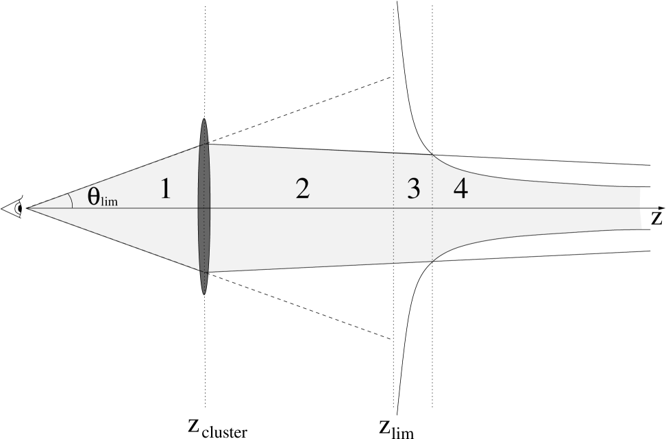
Figure 1: Schematic picture of the lensing situation. $z_{\rm lim}\ (m_{\rm lim})$ is the limiting redshift (magnitude) without the lensing cluster. The shaded area indicates the volume where the SNe are bright enough to be detected and are visible within the field. Compare the four different areas 1-4 to the four different distinguishable $z$-bin ranges of Fig. 2

Figure 2: Number of SNe detected per year in redshift bins of $\Delta z=0.05$. Area 1 at redshifts smaller than the cluster redshift, $z_{\rm cl}$, area 2 between the lens and $z_{\rm lim}$, area 3 where the visible field limits the number of SNe and area 4 where the magnification is the limitation. The dashed line shows the number count without the lens and the solid line with a NFW lens redshift of $z_{\rm cl}=0.2$ and a field-of-view of 16 square arcminutes.

3 The method

The number of SNe that can be detected is found by integrating the number density of supernovae over the volume swept out by the FOV. Naturally, we count all SNe in this volume that are bright enough to be observed, either intrinsically or after having been magnified by lensing, see Fig. 1. The trumpet shaped shaded area beyond $z_{\rm lim}$ indicates where the SNe are magnified above the detection threshold, $m_{\rm lim}$. This figure is to be compared to Fig. 2, which is an example of a typical set of parameters for Type Ia SNe and a NFW lens and shows the number of detected SNe, $N$, per year and redshift bin $\Delta z=0.05$. The shaded areas (volumes) denoted 1-4 in Fig. 1 also have counterparts here. Up to the lens redshift, $z_{\rm cl}$ (at 0.2 here), there should be no difference between the cases with and without the lens (area 1). Beyond the lens, there is a region where the spreading of the field diminishes the area compared to the case with no lens (area 2), from $z_{\rm cl}$ to $z_{\rm lim}$. Beyond $z_{\rm lim}$ there is a small area where the visible field still is the limiting factor to the number count (area 3). Finally, the magnification is limiting in area 4. Under specific circumstances, e.g.  if the lens is very massive or at low redshifts and the FOV is small, another effect might become important. As indicated above, there are no primary images inside the Einstein radius. In all our considered models, primary images are much more numerous than secondary or tertiary, and in principle a situation can arise where $\theta_{\rm lim}<\theta_{\rm E}$ only giving secondary and tertiary images at this source redshift. This will lead to a decrease in the number count when many sources are affected and the effect can be seen in Fig. 9.

As multiple imaging is possible we have taken this into account by counting secondary and tertiary images that are bright enough as events independent of the primary image, resulting in a slightly higher rate. As indicated above this is a very small effect in all cases considered here.

3.1 Supernova rates, types and magnitudes

We have concentrated our study on Type Ia and Type II supernovae. The Type II SNe are divided into three subclasses: IIn, IIp and IIL, with abundances of 0.02, 0.3 and 0.3 relative to the total core-collapse (cc) SN rate (IIn+IIp+IIL+Ibc+87a-like) following the predictions in Dahlén & Fransson (1999), see Fig. 3. In order to study the power of galaxy clusters as GTs we have neglected the intrinsic brightness dispersion of the supernovae as well as extinction. Thus, the magnitude dispersion considered in this work stems only from gravitational lensing. For comparison, the intrinsic properties (from Richardson et al., 2002) of SNe are listed in Table 1.

We have also taken the conservative viewpoint that the SNe are not discovered at maximum by adding 0.5 magnitudes to the absolute magnitudes in the table. This has the same effect as decreasing the limiting magnitude of the telescope by 0.5 magnitudes.

The simple identification of areas 1-4 in Figs. 1 and 2 is not possible in the case of our Type II SN plots. This is due to the fact that they have different luminosities and will be seen out to different $z_{\rm lim}$ (defined in Fig. 1). This instead gives rise to three peaks (at most) in the $N/{\rm yr}/\Delta z$ vs. $z$ plots for Type II SNe as they show the sum of all three types considered.

Figure 3: Supernova rates versus redshift in bins of $\Delta z=0.05$. For core collapse SNe the plot shows IIn+IIp+IIL+Ibc+87a-like. The increasing time dilation of the SN rate with redshift is taken into account.The distribution includes neither lensing nor observational selection effects.

Table 1: Supernova properties, assuming discovery at maximum luminosity in $B$-band. Type Ibc and 87a-like events are not considered but are listed for completeness.

Type	Rel. cc fraction	Abs. mag. $M$	Disp. $\sigma_{\rm M}$
IIn	0.02	-18.78	0.92
IIp	0.3	-16.61	1.23
IIL	0.3	-17.80	0.88
Ibc	0.23	-17.92	1.29
87a-like	0.15	-	-
Ia	0	-19.17	0.16

3.2 Cluster models

We use two different models for the clusters, the singular isothermal sphere (SIS) and the Navarro-Frenk-White profile (NFW) obtained in N-body simulations (Navarro et al., 1997) on which we will focus. The large lens masses considered here seem to be better fitted by the NFW profile (Li & Ostriker, 2002) but we will see in Sect. 4 that they do not differ much for the cases we consider.

There is also an ongoing debate on whether the dark matter halos are centrally cuspy or possess a roughly constant density core. The issue is not settled but there is some evidence of cuspy central regions on cluster scales which is what we have assumed in this paper (see e.g. Dahle et al., 2002).

For a description of the lensing properties of the SIS, see e.g. Schneider et al. (1992, Ch. 8.1.4). The SIS only has primary and secondary images as the tertiary image always is infinitely faint.

Gravitational lensing by NFW halos is well described in Wright & Brainerd (2000) and we refer to that paper for further reading. To find the parameters for a specific cluster mass and redshift we use the Fortran 77 code charden.f available on the homepage of Julio Navarro. The NFW profile produces both primary, secondary and tertiary images.

To meaningfully compare the results for SIS and NFW we have assumed $M_{\rm vir}$, the mass within the virial radius, to be equal for both of them. The virial overdensity used to obtain the virial radius is computed using the results found in (Bryan & Norman, 1998) which is a fit to the calculation in (Eke et al., 1996). However, the Einstein radii of a NFW and a SIS halo of equal virial mass will be quite different. For a $1.4\times 10^{15}\ h^{-1}$ M_⊙ halo at $z_{\rm cl}=0.2$, $\theta_{\rm E}^{\rm SIS}\sim 2\theta_{\rm E}^{\rm NFW}$ for source redshifts between 1.5 and 4. This difference in ER does not affect the results strongly as is seen e.g. in Fig.11. In Figure 4 we have plotted the source redshift dependence of the Einstein radius, within which strong lensing effects occur, for two different $1.4\times 10^{15}h^{-1}$ M_⊙ NFW cluster redshifts. As can be seen, the ER has a weaker dependence on $z_{\rm s}$ for higher redshifts.

Figure 4: Redshift dependence of the Einstein radius, within which strong lensing effects occur, for two different cluster redshifts, $z_{\rm cl}$. The cluster virial mass is $1.4\times 10^{15}h^{-1}$ M_⊙.

3.3 Telescope and cluster parameters

The main reason for studying gravitationally magnified supernovae is that it might enable us to explore supernova explosions otherwise too faint to be detected by the search instruments currently used or being planned. Because these SNe are predominantly at very high redshifts we focus on the use of the largest wavelength optical filters and NIR for their discovery. We concentrate on the feasibility to discover magnified SNe in the $I$-, $Z$- and $J$-bands.

We are assuming a circular 16 sq. arcminutes field centered on the galaxy cluster. The considered solid angle is thus comparable to the foreseen FOV of NIRCam/JWST and slightly larger than the dimensions of the Advanced Camera for Surveys (ACS, 3$\aas@@fstack{\prime}$37 $\times$ 3$\aas@@fstack{\prime}$37), on HST where SN searches are currently conducted in $Z$-band by e.g. the GOODS team. Ground based NIR cameras on 8-m class telescopes with deep imaging capabilities in $J$-band like ISAAC/VLT (2$\aas@@fstack{\prime}$5′$\times$ 2$\aas@@fstack{\prime}$5), NIRI/Gemini (2′$\times$ 2′) or CISCO/Subaru (2′$\times$ 2′) are also contained within the maximum FOV considered. We also briefly consider searches in $I$-band where most of the efforts of the SCP and High-Z teams are concentrated, although with significantly larger FOV. K-corrections were calculated using the SNOC package (Goobar et al., 2002b).

Figure 5: Redshift reach as a function of limiting ($Z$-band) magnitude in the supernova search. For comparison, the ACS/GOODS transient survey has a limiting magnitude around $Z$=25.5.

We have investigated limiting magnitudes ranging from 22nd to 30th magnitude, reaching up to a limiting redshift $z_{\lim}\sim 4-5$ for some of the SN types considered. Primarily, we study the properties of quite heavy clusters of virial mass $1.4\times 10^{15}\ h^{-1}$ M_⊙ as GTs but we also briefly consider a cluster of mass $1.4\times 10^{14}\ h^{-1}$ M_⊙. Cluster redshifts between $z_{\rm cl}=0.2$ and $z_{\rm cl}=1.0$ were assumed.

4 Simulation results

4.1 Supernova searches in $Z$-band

First, we consider the case of observational programs such as the ongoing ACS/GOODS transient survey, comparing the potential gain in the discovery rate if the observations were done looking towards a heavy galaxy cluster. These search observations are done in $Z$-band, with an approximate limiting magnitude of 25.5 mag.

If nothing else is stated, the lens model we use is a NFW halo. Figs. 6 and 7 show the expected number of discoveries in a 16 sq. arcminutes field for Type Ia and Type II SNe respectively. In the Ia case, although the search becomes significantly deeper, the effect of spreading the field dominates, giving an overall decrease in the number count, relative to the case with no lens, of more than 30 % for the assumed $z$-dependence of the rates. The qualitative effect proves to be roughly independent of the lens redshift even though it is less severe for higher cluster redshifts. For the fainter Type II SNe, the effect is reversed at this limiting magnitude and more supernovae could be detected at redshifts far beyond the cutoff without the lens. The quantitative gain can be seen in Fig. 8 where the gain factor, $N_{\rm lens}/N_{\rm nolens}$, is shown as a function of limiting magnitude. At $m_{\rm lim}=25.5$, a factor of 1.5 to 1.6 is obtained depending on the cluster redshift. Since the simulations were quite time-consuming, some time was saved by not computing too many points in each plot. This gives the artificial non-smooth behavior seen in the figure. The dip at $m_{\rm lim}=24$ for $z_{\rm cl}=0.5$ originates from the fact that $z_{\rm lim}(m_{\rm lim}=24)\simeq 0.46$ for Type IIL SNe i.e. slightly less than the lens redshift implying that all SNe of this kind beyond the cluster are missed in our “standard candle” treatment. Increasing $m_{\rm lim}$ pushes $z_{\rm lim}$ above 0.5. Thus, a sudden rise is expected since the Type IIL SNe behind the lens that are sufficiently magnified are seen. If these SNe were not present, the curve would have followed the qualitative behavior of the $z_{\rm cl}=0.2$ curve, i.e. decreasing after $m_{\rm lim}\sim 24$.

Figure 6: Number of Type Ia SNe detected per year and $\Delta z=0.05$ vs. $z$ in the $Z$-band for various cluster redshifts, $z_{\rm cl}$. The FOV is 16 sq. arcminutes while the limiting magnitude is chosen to be what is currently used at ACS for the GOODS transient survey.

Figure 7: Number of Type IIn+p+L SNe detected per year and $\Delta z=0.05$ vs. $z$ in the $Z$-band for two different cluster redshifts, $z_{\rm cl}$. The FOV is 16 sq. arcminutes.

Figure 8: Gain factor of Type IIn+p+L SNe detected vs. $m_{\rm lim}$ in the $Z$-band for two different cluster redshifts, $z_{\rm cl}$. The FOV is 16 sq. arcminutes.

4.2 Supernova searches in $J$-band

Next, we consider the possibility of doing the searches at near-IR wavelengths, e.g. in $J$-band. In this discussion we ignore the observational difficulties of such a program, e.g. the rather long exposure times required to overcome the high sky noise due to atmospheric emission if a ground based search were to be attempted. Searching with NICMOS on HST would be an alternative. A limiting factor is the small size of the HgCdTe arrays.

To see what effect the FOV and different cluster masses have on the simulations we plot the gain factor vs. $\theta_{\rm lim}$ (defined in Fig. 1) for two different cluster masses and $z_{\rm cl}=0.2$ in Fig. 9. The aforementioned effect that for a small FOV it is possible to end up inside the Einstein radius where no primary images of sources at some specific distance are found can be seen for small $\theta_{\rm lim}$ for both clusters. Although $\theta_{\rm E}$ depends on the source redshift, the dependence is rather weak for the higher redshift range as already noted. Between $z=1.5$ and $z=4$ the Einstein radius changes by about 20% and is $\sim 0\aas@@fstack{\prime}3$ for the heavier of the two clusters as can be seen in Fig. 4.

Figure 9: Gain factor of Type IIn+p+L SNe detected vs. $\theta_{\rm lim}$ for two different cluster masses $M_{\rm cl}$ and $z_{\rm cl}=0.2$. The limiting magnitude is 26 for this plot, using the $J$-band.

Figure 10 shows a gain in the number count discernible by comparing the areas under the graphs with and without the lens. This is seen quantitatively in Fig. 11 as a factor $\sim 1.25$ at $m_{\rm lim}=26$ for both lens redshifts. Figures 10 and 11 also makes it quite clear that the difference between the NFW and SIS models is small. Again we see the dip at $m_{\rm lim}=24$ in Fig. 11. To continue the comparison; we see a quite large increase in the gain factor at $m_{\rm lim}\sim 24$ (max. at 23.5 to be precise) for the $z_{\rm cl}=0.2$ cluster, and therefore we display in Fig. 12 the distribution of these Type IIs in redshift space for $m_{\rm lim}=24$ showing a clear and large displacement of the distribution towards higher redshifts compared to the case with no lens. This would seem particularly interesting as $J=24$ is clearly within reach for 8-m class ground based telescopes. However, Fig. 13 reveals that the absolute number of SNe for this limiting magnitude is quite low. One important thing to note though is that the absolute numbers are uncertain since they depend strongly on the supernova rates which in turn are quite uncertain, especially for sources at higher redshifts.

Figure 10: Number of Type IIn+p+L SNe detected per year and $\Delta z=0.05$ vs. $z$ in the $J$-band. The cluster redshift is 0.5 and the FOV is 16 sq. arcminutes. This plot shows the small difference between the NFW and SIS profiles at this limiting magnitude.

Figure 11: Gain factor of Type IIn+p+L SNe detected vs. $m_{\rm lim}$ in the $J$-band for two different cluster redshifts, $z_{\rm cl}$. The small difference between NFW and SIS is also seen in this plot. The FOV is 16 sq. arcminutes.

Figure 12: Number of Type IIn+p+L SNe detected per year and $\Delta z=0.05$ vs. $z$ in the $J$-band for a cluster at $z=0.2$ and with a limiting magnitude of 24. The FOV is 16 sq. arcminutes.

Figure 13: Number of Type IIn+p+L SNe detected per year vs. $m_{\rm lim}$ in the $J$-band for two different cluster redshifts, $z_{\rm cl}$. The FOV is 16 sq. arcminutes and the distribution is cumulative

If we now study similar plots for Type Ia SNe we see a huge increase in the gain factor at small $m_{\rm lim}$ $\sim$22-23 in Fig. 14 for the $z_{\rm cl}=0.2$ cluster. Unfortunately this is not so exciting when comparing with Fig. 15 where we again see that the absolute numbers are quite low. However, in the region $23.5\lesssim m_{\rm lim}\lesssim 24.5$ the situation looks a bit more interesting for the nearer cluster.

Figure 14: Gain factor of Type Ia SNe detected vs. $m_{\rm lim}$ in the $J$-band for two different cluster redshifts, $z_{\rm cl}$. The FOV is 16 sq. arcminutes.

Figure 15: Number of Type Ia SNe detected per year vs. $m_{\rm lim}$ for two different cluster redshifts, $z_{\rm cl}$. The FOV is 16 sq. arcminutes and the distribution is cumulative.

4.3 Supernova searches in $I$-band

Finally, we briefly compare the results shown so far with the expectations from an $I$-band SN search, the currently favoured search filter for ground based high-$z$ supernova searches. Fig. 16 shows the expected benefit of heavy clusters as GTs at two redshifts for $I$- and $J$-band. The gain in the $I$-band is generally smaller in the interesting region where the gain is greater than one except maybe for a high redshift cluster. However, clusters this heavy at such high redshifts are very rare (Rosati et al., 2002). Again, the bumpy behaviour of the $z=1.0$ $J$-band graph is due to the effect described in Sect. 4.1 for Type IIL SNe.

Figure 16: Gain factor of Type IIn+p+L SNe detected vs. $m_{\rm lim}$. in the $I$- and $J$-bands for two different cluster redshifts, $z_{\rm cl}$. The FOV is 16 sq. arcminutes.

5 Discussion

As stated above we have treated all SNe as standard candles. This perhaps crude assumption when applied to Type II SNe might appear plausible because one can assume approximately equally many SNe brighter than average as fainter for each SN type. This could then be assumed to average out. However, the effect of adding a dispersion is not trivial since it will affect the lensed and the unlensed case differently. The magnification will boost the faint end tail, thereby adding from this tail supernovae in area 2 of Fig. 1 to the number count. The effect on the unlensed case will be to add some SNe beyond and remove some SNe prior to $z_{\rm lim}$ but with a larger volume for the ones beyond. The effect will also depend on the differential SN rate, especially around $z_{\rm lim}$. A more careful investigation should of course include the SN brightness dispersion.

A more robust justification is found by studying the magnification as a function of the impact parameter, see Fig. 17. For a $1.4\times 10^{15}\ h^{-1}$ M_⊙ NFW cluster at $z_{\rm cl}=0.2$ and a source at $z=2.0$ it is seen that within 1$\arcmin$ of the cluster core, the magnification exceeds one magnitude, approximately the intrinsic dispersion of the Type II SNe considered, see Table 1. Thus, within this radius the magnification dominates the magnitude dispersion for this lens-source configuration. The situation does not change much for sources in the most interesting regions where the SN rate is high. However for lighter clusters we see that the approximation becomes worse. Similarly, extinction losses have been neglected. Thus, the net benefit of gravitational lensing is somewhat underestimated, as GTs would certainly enhance the detectability of extincted supernovae.

Figure 17: Magnification as a function of the impact parameter in the lens plane for a source at $z=2$. The lens redshift is 0.2.

In Fig. 17 we can also identify the regions where secondary and tertiary images appear. Tertiary images show up in the innermost regions up to the first big dip. Secondary images are located between the two dips and outside the second dip (the locus of the Einstein radius) there are only primary images. Although not obvious from Fig. 17, in all our considered models primary images are much more abundant for larger fields-of-view and roughly make up about 95 % of the images. However, the fraction of secondary and tertiary images is larger for lower redshift clusters (and also for SIS clusters which are more efficient image-splitters) since we then look at the more central parts of the cluster.

We have only studied spherically symmetric clusters which of course is an oversimplification since clusters undoubtedly have substructure in the form of cluster member galaxies. To see in more detail how a specific cluster can affect the searches, a better way is to follow the example in Saini et al. (2000) and use a more sophisticated lens model.

The adopted cluster masses in this work, $\sim 10^{15}\ h^{-1}$ M_⊙, are consistent with virial and lensing mass estimates of X-ray luminous clusters at $z\sim 0.2-0.3$ (see Irgens et al., 2002, and references therein).

Finally, since we have left out Type Ibc (and 87a-like) SNe we have underestimated the total number of SNe that would be detectable.

6 Conclusions

Observations pointing behind massive heavy galaxy clusters at redshifts $z=0.2-0.5$ may be a useful way to enhance the detectability of very high-$z$ supernovae. For the considered supernova rates, the most interesting effects show up for core-collapse SNe in searches at limiting magnitudes $m_{\rm lim}\sim 25-26.5$ mag where the detection rate could be significantly enhanced and where the absolute number of detectable events is considerable. However, the SN rates at high-$z$ and thus also the absolute numbers are quite uncertain. The relative gain, which is less sensitive to the SN rates, peaks at lower limiting magnitudes of $\sim$24 where the number of detections could increase by up to a factor 3 and by a much larger factor at the highest redshifts. For programs such as the GOODS/ACS transient survey, the discovery of supernovae beyond $z\sim 2$ may be significantly increased with the aid of GTs. This technique may be used to probe the cosmic star formation rate at very high redshifts where there is significant controversy (see e.g. Lanzetta et al., 2002) although this requires good knowledge of the cluster properties such as mass and density profile. When interpreting the measured rates of distant SNe as well as their apparent brightness, special care must be taken so that magnification effects from GTs are properly accounted for. The potential bias increases with the central wavelength of the filter used for the supernova search, due to the enhancement of acceptance for very redshifted sources. For extremely deep observations $m_{\rm lim}>27$ mag or for very bright SNe (e.g. Type Ia) the competing effect of field reduction dominates and fewer supernovae are likely to be discovered behind foreground clusters. However, the most important effect is that the detection rate at high redshift could be significantly enhanced when there is an intervening cluster acting as a gravitational telescope.