Physics Fundamentals of Luminous Accretion Disks Around Black Holes

Abstract

These lectures provide an overview of the theory of accretion disks with application to bright sources containing black holes. I focus on the fundamental physics of these flows, stressing modern developments and outstanding questions wherever possible. After a review of standard Shakura-Sunyaev based models and their problems and uncertainties, I describe the basic principles that determine the overall spectral energy distribution produced by the flow. I then describe the physics of angular momentum transport in black hole accretion disks, stressing the important role of magnetic fields. Finally, I discuss the physics of radiation magnetohydrodynamics and how it might affect the overall flow structure in the innermost regions near the black hole.

1 Introduction

Accretion disk theory was developed in a flurry of activity in the early 1970’s in a series of important, seminal papers [95, 102, 88, 75, 72, 90, 38, 103]. It has met with considerable success in explaining the observations we see in a number of classes of accretion-powered sources, particularly cataclysmic variables. However, it does a rather poor job of predicting and explaining the observations of black hole sources, both in the context of X-ray binaries and active galactic nuclei. This is particularly disappointing in view of the fact that much of the early development of the theory was done with this application in mind. Accretion disk theory has always suffered from a severe flaw: angular momentum transport and energy dissipation in observed flows must be due to nonlinear physics (“turbulence”), and this problem is swept under the carpet by parameterizing it away in terms of an anomalous “viscosity”. Over the past thirty years, this sad state of affairs has persisted, although a major breakthrough was made in 1991 with the discovery that the magnetorotational instability (MRI) might be a generic source of turbulence in disks [16, 52]. Thanks to this insight and the increasing sophistication and capabilities of numerical simulations, we are now beginning to address virtually all aspects of accretion disk theory from first principles physics. The coming decade should see such models applied to observation, finally getting us to the point where we are able to test the basic physics, and not fudge factors. We are therefore living and working in an exciting time!

In these lectures, I will give an overview of the current state of the theory. Although I will be discussing accretion disks in some generality, I will for the most part concentrate on disks around black holes. Unless explicitly noted, I will always use Newtonian physics, even though the flows around black holes necessarily involve relativistic effects, both special and general. I do this purely for the sake of pedagogy. Relativity is not difficult - in fact, it is the easy part of black hole accretion disk physics. As we will see, all the really nasty (albeit interesting!) issues lie in the radiation and plasma physics, and the basic principles involved here are most quickly understood within a Newtonian framework. Almost everything I discuss has been worked out in full general relativity somewhere in the literature, and I give references to such work wherever possible.

Many good textbooks exist which discuss aspects of the basic physics of accretion disks, e.g. [42, 67, 104], and the reader is encouraged to consult them for a more elaborate treatment of the now-standard ideas. As I already mentioned, however, many of these ideas will soon be superseded by much more sophisticated models based on real physics. The best overview of the MRI is the review by Balbus & Hawley [19], although some advances have taken place since that article was written.

I will begin in section 2 with a brief overview of standard models based on the Shakura-Sunyaev $\alpha$-prescription for the anomalous stress that must exist in these flows, as these are still the models that people use for comparison to observational data. I will focus on recent developments in this area, including the role of advection in “slim disks”, the role of torques exerted across the innermost stable circular orbit, and the vertical transfer of mechanical energy out of the disk into a corona. In section 3, I will discuss the calculation of photon spectra from these models. I will then return to first principles in section 4 by examining the basic origin of anomalous angular momentum transport in disks, emphasizing the role of magnetic fields. Finally, in section 5, I will discuss the role that radiation magnetohydrodynamics may play in determining the dynamics and thermodynamics of the innermost regions of the flow, where most of the observed radiation is thought to originate.

2 Shakura-Sunyaev Based Models

Most, but not all, models of accretion-powered sources assume that rotation is an important source of dynamical support in the accretion flow. Gas accreting onto a compact object from an orbiting companion star is endowed with considerable angular momentum arising from the orbital motion of the binary itself. The huge dynamic range in radii between the fuel source and the radius of the central object in young stellar objects (YSO’s) and active galactic nuclei (AGN) also strongly suggests that rotation is important. If material at large radii has some nonzero angular momentum with respect to the central object, and if that angular momentum is conserved on the way in, then the material is likely to become rotationally supported. This is simply because centripetal acceleration then depends on distance $R$ from the rotation axis as $R^{-3}$, steeper than the $R^{-2}$ dependence of gravitational acceleration. (This statement neglects general relativistic effects. Sufficiently close to the event horizon, the gravitational acceleration will dominate all rotational support and even material with conserved angular momentum will flow inward all the way to the singularity.) Direct observational support for the existence of rotationally supported accretion flow structures exists in many images of YSO disks and in the maser disk of the low luminosity AGN NGC 4258 [82].

Angular momentum will generally not be conserved in the flow, and the mechanisms of outward angular momentum transport and how they are connected to the conversion of orbital mechanical energy into other forms are central to understanding how accretion power works. Ordinary fluid viscosity is far too weak to be a significant factor, and something else must exert torques (either internal or external, or both) on the flow.

Virtually all models that actually attempt to make contact with the observations are based on a phenomenological prescription of a (vertically-averaged) anomalous internal stress introduced by Shakura & Sunyaev in 1973 [102]:

$$\tau_{R\phi}=\alpha P,$$ (1)

where $P$ is a vertically-averaged pressure. Many workers in the field continue to think about this stress as a form of “viscosity”, and the stress prescription is often explicitly introduced as exactly that! (As we shall see below, such naive thinking is very dangerous and can be extremely misleading.) For example, a commonly used modification of the Shakura-Sunyaev prescription is to assume a kinematic viscosity of the form

$$\nu\simeq\alpha c_{s}H\simeq\alpha c_{s}^{2}/\Omega_{\rm K},$$ (2)

where $c_{s}^{2}\simeq P/\rho$ is the vertically averaged sound speed (and $\rho$ is a vertically averaged density), $H=H(R)$ is the vertical half-thickness of the disk, and $\Omega_{\rm K}$ is the angular velocity of test-particle circular orbits (the “Keplerian” angular velocity). When inserted into the standard viscous form of the stress, this gives

$$\tau_{R\phi}=\rho\nu R\xdrv{\Omega}{R}=\alpha P{R\over\Omega_{\rm K}}\xdrv{\Omega}{R}.$$ (3)

Here $\Omega=\Omega(R)$ is the actual angular velocity in the flow, which may differ from $\Omega_{\rm K}$ if the flow is not completely geometrically thin. If $\Omega\sim\Omega_{\rm K}$, then within factors of order unity, equation (3) gives the same stress as equation (1). The only difference is that the stress now depends explicitly on the shear in the flow, just as an ordinary viscous stress would. This simple change completely alters the mathematical character of the critical point problem in stationary advective flows [12], but it is not clear that any of this is real.

Yet another uncertainty that has plagued black hole accretion disk models with Shakura-Sunyaev stress prescriptions from the very beginning is what pressure (gas or radiation or…?) to stick into equations (1) or (3) when radiation pressure is comparable to or greater than gas pressure. This occurs in the central parts of standard disk models around black holes accreting at anywhere near the Eddington rate (see eqs. [76]-[77] below), right where most of the power is generated. Moreover, the first thing that one would try (just inserting the total, gas plus radiation, pressure) leads to a disk that cannot be stationary because it is thermally and “viscously” unstable [72, 103].

Let us briefly trace the argument for the radiation pressure driven thermal instability, which acts on a much faster time scale $\sim 1/(\alpha\Omega)$ in geometrically thin disks than the “viscous” instability which acts on the radial flow time scale $\sim R^{2}/(H^{2}\alpha\Omega)$. Assuming that cooling of the disk proceeds through radiative diffusion, the local emergent flux at radius $R$ is given by

$$F^{-}\sim{acT^{4}\over\tau},$$ (4)

where $a$ is the radiation density constant, $c$ is the speed of light, $T$ is a measure of the disk interior temperature, and $\tau$ is half the total vertical optical depth. The inner parts of black hole accretion disks have opacities that are generally dominated by electron scattering, so $\tau\sim\kappa_{\rm T}\Sigma/2$, where $\Sigma$ is the surface density of the disk, which is constant on these time scales very much less than the radial flow time scale. The Thomson opacity $\kappa_{\rm T}$ is also constant, being independent of temperature provided there is already sufficient ionization (and there is), so the optical depth is independent of temperature and the cooling rate per unit area is $F^{-}\propto T^{4}$. Note that I have made the usual assumption here that $F^{-}$ is a real heat flux and does not involve other forms of energy.

The dissipation rate per unit area is

$$F^{+}\sim RH\tau_{R\phi}\xdrv{\Omega}{R}.$$ (5)

Vertical hydrostatic equilibrium implies that the disk half thickness $H\sim 2P/(\Omega_{\rm K}^{2}\Sigma)$, so that eq. (5) becomes

$$F^{+}\sim{2RP\tau_{R\phi}\over\Omega_{\rm K}^{2}\Sigma}\xdrv{\Omega}{R}.$$ (6)

In the radiation pressure dominated inner region, $P\simeq aT^{4}/3$, so that equations (6) and (1) or (3) imply that $F^{+}\propto T^{8}$! Hence a perturbative increase in temperature increases both the local cooling and heating rates, but the heating rate increases much faster, leading to a thermal runaway.

Such thermal (and “viscous”) instabilities arising from opacity variations in hydrogen ionization zones rather than radiation pressure have been applied with considerable success to understanding the outburst behavior of dwarf novae (e.g. [89]) and soft X-ray transients (e.g. [65]). The reality of these instabilities in radiation-pressure dominated zones has never been established, however. It has been argued [98] that the stress should be proportional to the gas pressure only, in which case $\tau_{R\phi}\propto\rho T\propto\Sigma^{2}\Omega_{\rm K}^{2}T/(4P)\propto T^{-3}$ in the radiation pressure dominated inner zone. This implies that $F^{+}$ depends only linearly on temperature, producing a thermally (and in fact “viscously” as well) stable flow. We will examine this argument in section 5 below. In addition, we will look at how radiation magnetohydrodynamic instabilities might affect thermal instabilities in accretion flows.

Observationally motivated models of accretion flows generally start with the assumption that the flow is stationary and axisymmetric about the rotation axis, even though whatever is responsible for the anomalous angular momentum transport must almost certainly involve time-dependent, non-axisymmetric fluctuations. (Time-dependent models are often constructed to model the response of the disk to thermal and “viscous” instabilities.) Another simplifying assumption is that vertically-integrated flow equations provide a reasonably accurate description of the behavior of conserved quantities, even if the flow is not very geometrically thin. The resulting steady-state conservation laws are those for mass,

$$\dot{M}=4\pi RH\rho v,$$ (7)

radial momentum,

$$\rho v\xdrv{v}{R}=\rho(\Omega^{2}-\Omega_{\rm K}^{2})R-\xdrv{P}{R},$$ (8)

angular momentum,

$$\dot{M}\xdrv{\ell}{R}=\xDrv{(4\pi R^{2}H\tau_{R\phi})}{R},$$ (9)

and energy,

$$-4\pi RF_{\rm adv}\equiv\dot{M}\left[\xdrv{U}{R}+P\xDrv{\left({1\over\rho}\right)}{R}\right]=4\pi R^{2}H\tau_{R\phi}\xdrv{\Omega}{R}+2\pi R(2F^{-}).$$ (10)

Here $\dot{M}$ is the constant accretion rate through the flow, $R$ is the distance from the rotation axis, $v(R)$ is the inward radial flow speed, $\ell(R)$ is the angular momentum per unit mass, $U(R)$ is the internal energy per unit mass, and $F^{-}(R)$ is the energy flux leaving the flow on each of the two vertical surfaces.

Note that the anomalous stress $\tau_{R\phi}$ is assumed to enter the angular momentum and energy equations in exactly the same way as an ordinary fluid viscous stress: torques are exerted in a dissipative fashion. This need not be the case. External torques exerted on the disk by a global, ordered magnetic field in a magnetohydrodynamical (MHD) wind can in principle extract energy and angular momentum in precisely the right ratio necessary to allow material to accrete with no dissipation [31]. The disk can be ice cold and still accreting! Because of possibilities like this, I have been careful to call $F^{-}$ an energy flux and not a heat flux. Even if internal turbulence is responsible for angular momentum transport, it is still not clear that all the accretion power should be converted into heat. Instead, some of that power may be converted into bulk kinetic and magnetic energy, and $F^{-}$ must include these non-radiative contributions.

Equations (8) and (10) differ from those of standard geometrically thin accretion disk theory (e.g. [102]) by the inclusion of advective and radial pressure support terms which have received huge theoretical attention in recent years in the guise of advection dominated accretion flows (ADAFs, [2], [86]). In the absence of these effects, one gets the standard equations of thin disk theory, i.e. that the angular velocity is Keplerian,

$$\Omega(R)=\Omega_{\rm K}(R),$$ (11)

and local internal dissipation is balanced entirely by local vertical cooling,

$$F^{-}=-RH\tau_{R\phi}\xdrv{\Omega_{\rm K}}{R}.$$ (12)

The angular momentum equation (9) can be integrated from an inner radius of the flow $R_{\rm in}$ (usually taken to be the innermost stable circular orbit, or ISCO, radius for black hole accretion disks) out to an arbitrary radius $R$ to give

$$\dot{M}(\ell-\ell_{\rm in})=4\pi R^{2}H\tau_{R\phi}-4\pi R_{\rm in}^{2}H_{\rm in}\tau_{R\phi{\rm in}}.$$ (13)

Combining this with the local energy balance condition (12) for geometrically thin disks allows us to write down an expression for the emergent flux which is independent of the anomalous stress throughout most of the flow,

$$F^{-}={3GM\dot{M}\over 8\pi R^{3}}\left[1-\left({R_{\rm in}\over R}\right)^{1/2}+{4\pi R_{\rm in}^{2}H_{\rm in}\tau_{R\phi{\rm in}}\over\dot{M}(GMR)^{1/2}}\right].$$ (14)

This is the most beautiful result of standard accretion disk theory: that steady state accretion disks have an emergent flux that is independent of the details of the anomalous stress. Of course, accretion flows around black holes are observed to vary on all sorts of time scales, so steady state may not be a good assumption. Moreover, there is still a dependence on the stress $\tau_{R\phi{\rm in}}$ at the inner edge of the flow. Until recently, this stress was almost always assumed to vanish near the ISCO, due to the fact that the inward transonic flow inside this point was presumed to rapidly decouple from the disk. This assumption has been challenged recently [68, 44], and the physics of angular momentum transport near the ISCO has since received considerable theoretical scrutiny. We will examine this further in section 4 below, and for now, we will keep the inner stress in our equations.

Equation (14) can be integrated to give the total luminosity of the disk,

$$L=\int_{R_{\rm in}}^{\infty}2\pi R(2F^{-}){\rm d}R={GM\dot{M}\over 2R_{\rm in}}+(4\pi R_{\rm in}^{2}H_{\rm in}\tau_{R\phi{\rm in}})\Omega_{\rm in}.$$ (15)

This has a simple physical interpretation. The first term is the binding energy per unit mass of material at the inner radius, times the accretion rate. The second is the rate at which work is being done on the disk at the inner radius. By defining the accretion efficiency in the usual way, $\eta\equiv L/(\dot{M}c^{2})$, with $\eta_{SS}$ being the efficiency under the standard (Shakura-Sunyaev) assumption of a no-torque inner boundary condition and $\Delta\eta\equiv\eta-\eta_{\rm SS}$ being the additional efficiency due to the inner torque, equation (14) can be written in a physically appealing way (e.g. [7]),

$$F^{-}={3GM\dot{M}\over 8\pi R^{3}}\left[1-\left({R_{\rm in}\over R}\right)^{1/2}+\Delta\eta\left({R_{\rm in}\over r_{\rm g}}\right)\left({R_{\rm in}\over R}\right)^{1/2}\right].$$ (16)

Here $r_{\rm g}\equiv GM/c^{2}$ is the gravitational radius. (The full relativistic version of eq. [16] may be found in [7].) Note that the effects of the inner boundary on the flux decay with radius as $R^{-7/2}$, only slightly faster than the overall asymptotic decay of the flux at large radius, $\propto R^{-3}$.

So far we have been neglecting the advective terms in our conservation laws (7)-(10). If we include them, equation (14) becomes

$$F^{-}=\left(-{\dot{M}\ell\over 4\pi R}\xdrv{\Omega}{R}\right)\left(1-{\ell_{\rm in}\over\ell}+{4\pi R_{\rm in}^{2}H_{\rm in}\tau_{R\phi{\rm in}}\over\dot{M}\ell}\right)-F_{\rm adv}.$$ (17)

Advection, which becomes increasingly important as one moves inward in the flow, has two effects: the rotation profile is no longer Keplerian, and the orbital energy dissipated at any radius is partly advected (lost!) radially inward. The latter effect is evident from the last term in equation (17). The emerging energy flux $F^{-}$ is less than it would be if advection was not included.

For luminous accretion disks, advection starts to play a big role when the overall luminosity starts to get above some fraction ($\sim 0.3$ in standard models) of the Eddington luminosity L_Edd. The flow is then geometrically thicker, becoming a “slim” or “thick” accretion flow. Such flows are thermally and “viscously” stable [1, 4], because $F_{\rm adv}$ has a temperature dependence strong enough to beat the temperature dependence of $F^{+}$. The radial and vertical structure of these flows is no longer decoupled, and the emergent flux $F^{-}$ now depends on the very uncertain assumptions that are usually made to solve for the vertical structure. For a discussion of the fully relativistic equations of advective accretion flows, see e.g. [3], [5], [92], and [26]. Fully relativistic models of optically thick, “slim” accretion disks have been constructed in [27]. Models of hyper-Eddington accretion flows onto stellar mass black holes relevant for gamma-ray burst models have also been constructed [93]. By far and away most of the energy dissipated in such flows is advected into the black hole until the accretion rate exceeds $\sim 10^{-2}$ M_⊙ s^-1, where neutrino losses can cool the gas on the flow time scale.

Before leaving this section, I should mention the considerable attention that has been devoted recently to optically thin, radiatively inefficient ADAF solutions around black holes. Because we are focusing on luminous accretion flows here, I will have little to say about these solutions, but it is important to recognize that they may nevertheless arise over certain ranges of radii even in otherwise luminous flows. In particular, it is noteworthy that such flow solutions exist that are thermally and “viscously” stable over much the same range of accretion rates that geometrically thin, optically thick disk solutions exist (e.g. [33]), and it is not clear why nature should choose one flow solution over the other. The presence or absence of an inner ADAF flow might explain the different spectral states observed in black hole X-ray binaries [39]. One should bear in mind, however, that all the models discussed in this section are based on the $\alpha$ stress prescription, and it is fair to say that the microphysics of optically thin ADAFs is even more poorly understood than that of optically thick flows (e.g. [25], [96]).

3 Spectral Formation

As we saw in the last section, if we neglect the effects of advection, then the energy flux emerging from each face of a stationary accretion disk can be written

$$F^{-}(R)={3GM\dot{M}\over 8\pi R^{3}}{\cal I}_{a/M}(R/r_{\rm g}),$$ (18)

where ${\cal I}_{a/M}(x)$ is a function which in full general relativistic treatments depends on the spin parameter $a/M$ of the hole but still approaches unity at large radii. In standard models with a no-torque inner boundary condition, ${\cal I}_{a/M}$ also vanishes at the ISCO, but as we have seen, this need not be the case. Once again, let me remind the reader that although $F^{-}$ is usually assumed to be the emerging radiation flux from the disk surface, this need not be the case. It is actually the total energy flux, and may include contributions from magnetic and bulk kinetic energy. We will return to this point shortly, but for now, let us make the standard assumption that $F^{-}$ really does represent an emerging radiation flux.

What, then, is the emerging spectral energy distribution? An observer here on earth, viewing the disk at a distance $d$ away at an inclination angle $i$ to the rotation axis, will measure a spectral energy flux

$$F_{\nu}={\cos i\over d^{2}}\int_{R_{\rm in}}^{R_{\rm out}}2\pi RI_{\nu}(R,i){\rm d}R,$$ (19)

where $I_{\nu}$ is the angle (limb darkened or brightened!) and radius-dependent local emergent specific intensity, and we have introduced a finite outer radius $R_{\rm out}$ to the disk. (Once again, we are using Newtonian physics here, and neglecting e.g. Doppler shifts, gravitational redshifts, the gravitational bending of light rays, and the relativistic proper emitting area, but these are all straightforward to account for using relativistic “transfer functions”, e.g. [34, 108].)

The simplest (and therefore most often used!) way of estimating the shape of the spectrum is to just naively assume that each annulus radiates like an isotropic local blackbody, i.e. $I_{\nu}(R,i)=B_{\nu}[T_{\rm e}(R)]$, where $B_{\nu}$ is the Planck function with temperature given by the effective temperature determined from equation (18), $T_{\rm e}(R)=[F^{-}(R)/\sigma]^{1/4}$. If, say, the radial dependence of the emerging radiation flux can be approximated as a power law, $F^{-}(R)\propto R^{-\beta}$, then a simple change of integration variable to $x\equiv h\nu/(kT)$ implies that the shape of the observed spectrum is given by

$$F_{\nu}\propto\nu^{3-8/\beta}\int_{h\nu/(kT_{\rm ein})}^{h\nu/(kT_{\rm eout})}{x^{8/\beta-1}{\rm d}x\over e^{x}-1}.$$ (20)

As one would expect, at low frequencies satisfying $h\nu\ll kT_{\rm eout}$ we simply end up with $F_{\nu}\propto\nu^{2}$ (the Rayleigh-Jeans portion of the spectrum emitted by the outermost annulus), while at high frequencies satisfying $h\nu\gg kT_{\rm ein}$ we have $F_{\nu}\propto\nu^{3}\exp[-h\nu/(kT_{\rm ein})]$ (the Wien portion of the spectrum emitted by the innermost annulus). In between, for $kT_{\rm eout}\ll h\nu\ll kT_{\rm ein}$, the observed spectrum is a superposition of blackbodies from many different radii, producing a power-law spectrum $F_{\nu}\propto\nu^{3-8/\beta}$. Now, at large radii, equation (18) implies that $\beta=3$, giving the famous result that $F_{\nu}\propto\nu^{1/3}$ for a multi-temperature blackbody accretion disk.

There are many ways in which this standard result can be modified. One possibility is that energy liberated at small radii in the flow is reprocessed by the disk at larger radii. By way of illustration, consider a source of luminosity $L_{\star}$ located on the rotation axis at height $H_{\star}$ above the equatorial plane. Figure 1 illustrates the geometry of the problem.

Figure 1: Illumination geometry for a source on the symmetry axis at height $H_{\star}$ above the equatorial plane. The angle $\alpha$ between the disk normal and the incoming light ray is simply $\pi/2-(\beta+\theta)$, where $\theta$ is the angle between the tangent to the local disk surface and the equatorial plane, and $\beta$ is the angle between the illuminating light ray and the equatorial plane. For large $R$, $\beta$ and $\theta$ are both small angles, with $\beta\simeq(H_{\star}-H)/R$ and $\theta\simeq{\rm d}H/{\rm d}R$.

Neglecting general relativistic effects, in particular light bending, the irradiating flux on the outer disk at radius $R$ will be given by

$$F_{\rm irr}={L_{\star}(1-a)\over 4\pi R^{2}}\cos\alpha,$$ (21)

where $a$ is the albedo of the outer disk, averaged over the illuminating spectrum, and $\alpha$ is the angle between the disk normal and the incoming light ray. Taking the illuminating radius $R$ to be much larger than the local disk height $H$, the source height $H_{\star}$, and also ${\rm d}H/{\rm d}\ln R$, then a little trigonometry gives

$$F_{\rm irr}={L_{\star}(1-a)\over 4\pi R^{2}}\left({H\over R}\right)\left(\xdrv{\ln H}{\ln R}-1+{H_{\star}\over H}\right).$$ (22)

For a source located near the equatorial plane, e.g. the surface of the inner disk itself, we have $H_{\star}\ll H(R)$. Equation (22) then implies that significant reprocessing will only occur if the outer disk geometry flares up, with $H/R$ an increasing function of $R$, or is warped [94]. In this case, proportionately more power is transferred to larger radii, and this decreases the value of $\beta$ and reddens the spectrum. Standard models of disks work in just this way, with $H\propto R^{21/20}$ and $R^{9/8}$ for the so-called “middle” and “outer” regions, respectively. This gives an irradiating flux approximately proportional to $R^{-2}$, which must therefore dominate the more rapidly decaying ($\propto R^{-3}$) local dissipation, and giving $F_{\nu}\propto\nu^{-1}$ (e.g. [42]).

For a source located far above the equatorial plane, with $H_{\star}\gg H(R)$, equation (22) gives an irradiating flux $\propto R^{-3}$, producing the same $F_{\nu}\propto\nu^{1/3}$ spectrum as a standard disk but with enhanced power. One way in which this might be done is by having a geometrically thick, hot corona or ADAF in the inner parts of the flow. General relativistic light bending can also produce a similar effect: an observer located on the outer disk can see the opposite side of the disk at an effectively high $H_{\star}$ [7]. This effect alone can produce significant additions to the locally dissipated power in the case of rapidly rotating Kerr black holes [35].

Even without reprocessing, the emergent spectrum can be affected by alterations in the radial distribution of the local radiative flux $F^{-}$. For example, if an inner torque across the ISCO produces a large increase in the accretion efficiency, equation (16) implies that a substantial range of inner radii could have $F^{-}\propto R^{-7/2}$, giving a spectral energy distribution from equation (20) of the form $F_{\nu}\propto\nu^{5/7}$, bluer than $\nu^{1/3}$! On the other hand, gravitational light bending from the much brighter inner disk enhances the amount of reprocessed flux at larger radii, giving $F_{\rm irr}\propto R^{-3}$ and enforcing a more usual $F_{\nu}\propto\nu^{1/3}$ spectrum at longer wavelengths [7].

Advection also alters the radial distribution of $F^{-}$, causing it to rise less steeply toward smaller radii because more of the accretion power is advected into the black hole rather than being radiated. This in turn implies that $F^{-}$ falls less steeply when moving out in radius, implying a redder spectrum than $F_{\nu}\propto\nu^{1/3}$ [115]. In fact, models of slim disks can give flux distributions as flat as $F^{-}\propto R^{-2}$, and equation (20) then gives $F_{\nu}\propto\nu^{-1}$ [121, 122, 81]. The global effect of advection on the spectrum is that the luminosity is less than you would expect for the given accretion rate, because advection necessarily reduces the radiative efficiency.

Most models of the vertical structure of accretion disks around black holes imply that local blackbody emission is likely to be a very poor approximation. The most serious problem with it is the neglect of electron scattering, which is often far greater than true thermal absorption opacity. Again, a crude approach to handling this has been used from the very beginning of accretion disk modeling [102], and that is to use a so-called local modified blackbody spectrum at each radius,

$$I_{\nu}={2B_{\nu}(T)\epsilon_{\nu}^{1/2}\over 1+\epsilon_{\nu}^{1/2}},$$ (23)

where

$$\epsilon_{\nu}={\chi_{\nu}^{\rm th}\over n_{e}\sigma_{\rm T}+\chi_{\nu}^{\rm th}}$$ (24)

is the photon destruction probability, with $\chi_{\nu}^{\rm th}$ being the thermal absorption coefficient, $n_{e}$ the electron number density, and $\sigma_{T}$ the Thomson cross-section.

The physics behind equation (23) lies in the idea that, once created by thermal emission processes, photons random walk out of the atmosphere. If absorption opacity is smaller than electron scattering opacity, this random walk does not destroy photons generated within an effective optical depth $\tau_{\rm eff}=(\tau_{\rm abs}\tau_{\rm T})^{1/2}$ of the surface, where $\tau_{\rm abs}$ is the true absorption optical depth and $\tau_{\rm T}$ is the Thomson depth. Assuming LTE and integrating the emission over this vertical layer immediately gives $I_{\nu}\sim B_{\nu}\epsilon_{\nu}^{1/2}$, in rough agreement with equation (23). Provided the accretion disk is effectively thick ($\tau_{\rm eff}>1$ at the frequency of interest), then the spectrum may be viewed as coming from a depth in the disk corresponding to $\tau_{\rm eff}=1$. As shown in Figure 2, the innermost regions of some black hole accretion disk models are not even effectively thick, however, and the observed spectrum is formed throughout the entire geometrical thickness of the disk. In such cases the spectrum will be directly sensitive to the assumptions that went into creating the entire vertical structure. Even when $\tau_{\rm eff}>1$, the spectrum will depend on the ambient densities and temperatures at the $\tau_{\rm eff}=1$ effective photosphere, and these will in turn depend on the vertical structure of the disk model.

Figure 2: The midplane effective optical depth as a function of radius in relativistic accretion disk models around a ten solar mass black hole with $L=0.3L_{\rm Edd}$ and $\tau_{R\phi}=\alpha P_{\rm tot}$, where $P_{\rm tot}$ is the total (gas plus radiation) pressure. Both Kerr ($a/M=0.998$) and Schwarzschild models are shown, and a no-torque boundary condition is assumed at the ISCO, which is why the curves rise upward at small radii. The effective optical depth is actually a function of frequency, and what is depicted here is an average using the Rosseland mean free-free absorption opacity. Solid and dashed curves assume $\alpha=0.1$ and 0.01, respectively. The lower anomalous stress of the latter implies higher surface density and higher effective optical depth in both the Kerr and Schwarzschild cases.

Note that the modified blackbody spectrum in equation (23) has $I_{\nu}\leq B_{\nu}(T)$. This makes sense, as deviations from blackbody imply that the disk is a thermodynamically less efficient radiator. Because it must still radiate the same total flux, the ambient gas temperature must be hotter than the effective temperature, and the resulting spectrum therefore extends to higher photon energies. When integrated over the disk, the spectral energy distribution must therefore flatten below the canonical $F_{\nu}\propto\nu^{1/3}$ as photons are redistributed to higher energies. These effects are illustrated in Figure 3, which compares stellar atmosphere calculations of relativistic disk spectra with the local blackbody assumption.

Figure 3: Spectral energy distributions of relativistic accretion disk models around a $1.25\times 10^{8}$ M_⊙ Kerr ($a/M=0.998$) hole, accreting at 0.25 M_⊙ yr^-1, viewed at 60^∘ from the rotation axis [62]. The dashed curve, which extends to the highest energies, assumes that electron scattering is coherent (Thomson scattering). The solid curve allows for the effects of Compton scattering. Compton downscattering pulls the high energy tail of the spectrum down, while Compton upscattering increases the spectral luminosity at lower energies. The dot-dashed curve is the spectrum that results from assuming blackbody emission at the local effective temperature at every radius, and is clearly a very poor approximation.

In addition to the effects of Thomson scattering on the spectrum, Compton scattering can also be important in hot disks. The net Compton heating rate of the plasma per unit volume is

$$n_{e}\sigma_{\rm T}c\left({h\bar{\nu}\over m_{e}c^{2}}-{4kT\over m_{e}c^{2}}\right)\left({4\pi J\over c}\right),$$ (25)

where $J$ is the frequency-integrated mean intensity of the radiation field,

$$J\equiv\int_{0}^{\infty}d\nu J_{\nu}={1\over 4\pi}\int_{0}^{\infty}d\nu\oint d\Omega I_{\nu},$$ (26)

and $\bar{\nu}$ is a specially defined average frequency,

$$\bar{\nu}\equiv{1\over J}\int_{0}^{\infty}d\nu\nu J_{\nu}\left(1+{J_{\nu}c^{2}\over 2h\nu^{3}}\right).$$ (27)

(The second term in parentheses in equation [27] represents the effects of stimulated scattering.) The Compton heating rate can be compared with the net heating rate from thermal absorption and emission. Assuming LTE, this is

$$c\int_{0}^{\infty}d\nu\chi_{\nu}^{\rm th}\left({4\pi\over c}\right)(J_{\nu}-B_{\nu}).$$ (28)

Defining the Thomson opacity as

$$\kappa_{\rm T}\equiv{n_{e}\sigma_{\rm T}\over\rho}$$ (29)

and the Planck mean opacity as

$$\kappa_{\rm P}\equiv{1\over\rho aT^{4}}\int_{0}^{\infty}d\nu\chi_{\nu}^{\rm th}\left({4\pi B_{\nu}\over c}\right),$$ (30)

we see on comparing equations (25) and (28) that Compton scattering will dominate the thermal coupling between gas and radiation if

$$\kappa_{\rm T}\left({4kT\over m_{e}c^{2}}\right)\mathrel{\hbox to0.0pt{\lower 3.0pt\hbox{$\mathchar 536\relax$}\hss}\raise 2.0pt\hbox{$\mathchar 318\relax$}}\kappa_{\rm P}.$$ (31)

If, in addition, the effective Compton $y$-parameter,

$$y_{\rm eff}={4kT\over m_{e}c^{2}}{\rm max}\left(\tau_{\rm T},\tau_{\rm T}^{2}\right),$$ (32)

exceeds unity, at the particular frequency of interest, then Compton scattering will modify the spectrum, either by downscattering if $h\nu>4kT$, or upscattering if $h\nu<4kT$. (In equation [32], $\tau_{\rm T}$ is evaluated at the $\tau_{\rm eff}=1$ surface.) Figure 3 illustrates these effects on the spectrum.

Numerous authors have attempted detailed calculations of the spectral energy distributions emerging from accretion disks around black holes using stellar atmosphere modeling at every radius of the disk (see e.g. [113, 71, 97, 106, 112, 107, 37, 63, 101, 64, 61, 62] for models in the AGN context). Many of these models fully incorporate general relativistic effects on the disk structure, and also include relativistic Doppler shifts, gravitational redshifts, and gravitational bending of light rays. These latter effects play an important role in smearing out atomic absorption and/or emission features in the spectrum, as illustrated in Figure 4. Many models also incorporate sophisticated treatments of the radiative transfer, Compton scattering, and non-LTE effects in the atomic level populations of numerous elements and ions.

Figure 4: Spectral energy distributions of accretion disk models around Kerr ($a/M=0.998$) black holes at fixed Eddington ratio viewed nearly face on, for various black hole masses: $10^{8}$ (top), $10^{7}$ (middle), and $10^{6}$ M_⊙ (bottom) [62]. Note the increased relativistic smearing of the Balmer and Lyman edges of hydrogen for higher black hole mass. This is because the temperature of the disk is lower at higher mass, so these features are formed closer to the black hole.

As sophisticated as these models are, however, they still rest on variants of the Shakura-Sunyaev anomalous stress prescription, and are subject to all the uncertainties we discussed above in section 2. Moreover, just as a stellar model must specify a distribution of nuclear energy generation, a model of the vertical structure of an accretion disk must specify the distribution of turbulent heating. The presence of turbulence in the disk also begs the question as to whether heat is transported radiatively, or whether bulk transport in the turbulence itself also plays a role. As we discuss below in section 5, standard assumptions often used to model the inner, radiation pressure dominated regions lead to equilibria that are convectively unstable [28], although it is far from clear how that convection would manifest itself in a flow that already requires turbulent angular momentum transport.

Perhaps the most serious question plaguing current Shakura-Sunyaev based spectral models is the partitioning of the dissipation within the optically thick and thin regions of the disk. There is widespread empirical evidence for the existence of Comptonizing hot plasma in both black hole X-ray binaries and AGN, and one possibility is that this plasma exists as a magnetized corona above the disk photosphere. After all, the turbulent convection zone of our own sun generates a hot corona, so why shouldn’t a turbulent accretion disk have one as well? (This is one version of including non-radiative energy in $F^{-}$.) Models have even been considered in which most of the turbulent dissipation is assumed to occur in the corona, and not in the disk interior [49]! If a substantial fraction of the accretion power is in fact dissipated outside the disk, then there are numerous consequences [114]: the disk becomes geometrically thinner and denser, more effectively optically thick, and more gas pressure dominated.

Accretion disk physics is uncertain enough, but the physics of the hot plasma that must exist in real sources is even more insecure. Whether or not the hard X-rays observed in black hole X-ray binaries or AGN are generated in a disk corona or elsewhere in the flow (e.g. an inner ADAF that we discussed at the end of section 2), some of these X-rays will illuminate the disk from the outside, and thereby be reprocessed.

One of the most interesting X-ray reprocessing features is fluorescent iron K$\alpha$ line emission. The great excitement surrounding this line is that in at least three sources (MCG-6-30-15 [116, 123, 41], Mrk 766 [78], and NGC 3516 [84, 120]), it is clearly observed to be relativistically broadened. The resulting line profile is a convolution of the spatial emissivity profile of the line with relativistic Doppler shifts, gravitational redshifts, and gravitational light bending [70]. In other words, the line profile gives us the unprecedented opportunity to map out the equatorial test-particle orbit structure in a black hole spacetime, assuming the emitting material (the disk) is geometrically thin.

The K$\alpha$ line is produced because hard X-ray photons with energies above the K-edge of iron can knock inner shell electrons out of the atom. The resulting ion is born in an excited state and can return to the ground state by having an L-shell electron drop down to the vacancy in the K-shell, emitting either a K$\alpha$ line photon or one or more Auger electrons. The strength of the resulting emission line is sensitive to the ionization state of iron in the outer layers of the disk. At low ionization levels, where both the K and L shells of most iron ions have no vacancies, the material is transparent to K$\alpha$ photons which then escape more or less freely from the disk once they have been created by X-ray fluorescence. Once iron is sufficiently ionized that vacancies in the L-shell start to appear (FeXVIII to FeXXIV), then a K$\alpha$ photon can resonantly scatter off the iron atoms, enhancing the probability of its destruction through the Auger process. The emerging line strength is therefore reduced. This continues until iron is sufficiently ionized that only FeXXV and higher is present. The K$\alpha$ line photons still resonantly scatter with such ions, but the Auger effect cannot happen because there are no L-shell electrons to be ejected. At very high ionization when iron is fully stripped and the recombination rate is small because of high temperatures, no photoionization can occur and the emission line disappears. For an excellent review of the physics of the iron K$\alpha$ line, see [40].

The energy powering the iron K$\alpha$ line emission comes from photoelectric absorption of X-rays above the iron K-edge. Such photoelectric absorption by iron and other heavy elements present in the disk is in fact an efficient means of converting illuminating X-ray power below $\sim 10$ keV into heat in the outermost layers of the disk [48, 73]. Figure 5 shows the albedo of an illuminated slab of material as a function of incident photon energy [77]. Below $\sim 10$ keV, most of the incident X-rays are absorbed due to photoionization of heavy elements, and the level of that absorption depends on the ionization state of the disk. Above $\sim 10$ keV, the albedo quickly rises to near unity as the incident X-rays are simply reflected back by Thomson scattering. This is widely believed to explain the characteristic upturn of the X-ray spectrum that is observed at these energies in both AGN and black hole X-ray binaries [85, 124], and is strong evidence for the presence of relatively cold material in these sources. (Note that especially in the case of AGN, however, this cold material need not be the disk, but instead could be gas much further out from the source.) At higher energies the albedo is again reduced to well below unity, independent of the ionization state of the slab, because X-rays are Compton downscattered and therefore lose energy.

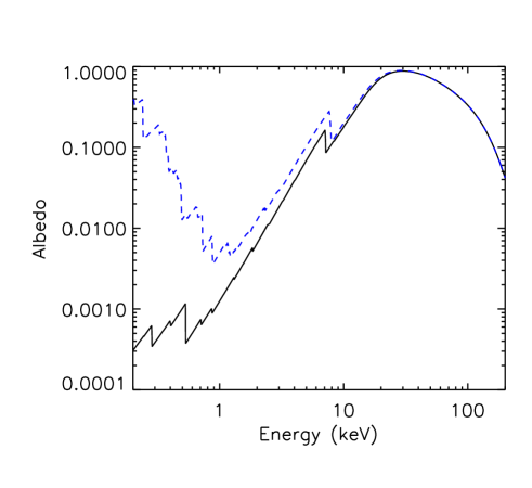
Figure 5: Energy-dependent albedo of an X-ray illuminated, cold slab with solar abundances, viewed at twenty degrees from the slab normal. The solid curve assumes the slab is neutral, apart from hydrogen and helium which are fully ionized. The dashed curve is for an ionized slab, with ionization parameter $\xi=100$. In both cases the illumination was assumed to be by a power-law spectrum with photon index -2 and exponential cutoff energy of 100 keV. (This figure was kindly generated by Shane Davis, courtesy of the XSPEC routines pexrav and pexriv [77].)

Just as the thermal emission spectra from accretion disks can depend sensitively on the details of the vertical disk structure, X-ray reprocessing and reflection features also depend on the assumptions one makes in describing the physics of the illuminated slab. Models that incorporate hydrostatic equilibrium produce surface temperature profiles containing a number of sharp discontinuities due to transitions between different regions of thermally stable material [87, 22], and the resulting reflection/fluorescent spectra are altered by this fact.

In addition to the very uncertain geometry of the illumination itself, one wonders whether even this treatment of the physics is enough. The bottom line of this section is that many aspects of our models of observed accreting black hole sources are fundamentally limited by uncertainties in the basic physics of the accretion flow itself. For the rest of these lectures we will switch gears and address this physics itself, explaining how to go beyond Shakura-Sunyaev type models.

4 The Physics of Angular Momentum Transport

A system with fixed total angular momentum in thermal equilibrium must be in a state of rigid body rotation [69]. This fact lies at the very heart of the way accretion disks work, because it shows that differential rotation is a source of thermodynamic free energy in the flow. As discussed long ago by Lynden-Bell & Pringle [75], one can always reduce the total rotational kinetic energy of an accretion disk by fixing its mass distribution and redistributing the angular momentum so that it is uniformly rotating. However, such a state is generally incompatible with mechanical equilibrium in the gravitational field of the central object, which requires that the angular velocity decrease outward. In this case, pairs of orbiting fluid elements moving with different angular velocities can lower their mechanical energy by shifting angular momentum from the element with higher angular velocity to the element with lower angular velocity [75]. This transports angular momentum outward through the disk, causing material to lose rotational support and flow in to regions of greater binding energy. This general behavior is simply the action of the second law of thermodynamics, and is entirely analogous to the one-way flow of heat from regions of high temperature to low temperature. Ordinary microscopic viscosity acts to transport angular momentum in exactly this fashion, but this is not sufficient for astrophysical accretion disks.

Some form of non-microscopic, “anomalous” angular momentum transport mechanism or mechanisms must therefore be at work, and it is important to recognize that it need not be the same in all accretion flows in the universe. Inherent in the Shakura-Sunyaev “guess” as to the form of the anomalous stress $\tau_{r\phi}$ is the existence of some form of turbulence in the flow: ideally a form of turbulence that is generated by the differential rotation itself. Turbulence is often, though not always, generated when a laminar flow is dynamically unstable to perturbations. These perturbations may be infinitesimal, so that the slightest touch of a feather will produce instability. The initial growth of the instability may then be understood from linearized equations about the equilibrium flow, which is then said to be linearly unstable. Linear equations are much easier to solve than nonlinear equations, and much of the theoretical work has therefore been devoted to linear instabilities. Understanding the response of the flow to nonlinear, finite amplitude perturbations is a lot harder, but there do exist laminar flows that are nonlinearly unstable even while being linearly stable. Of course to theoretically understand how a flow really changes in response to the development of even a linear instability requires a treatment of the nonlinear equations, which in practice is usually accomplished through numerical simulation.

The simplest way to examine the linear stability of a fluid is to infinitesimally perturb a fluid element locally and examine whether the forces exerted on the element act to return it to its original position. Stability criteria derived in this way are necessary, but not sufficient because it is also possible for the global structure of the flow to produce instabilities. Unfortunately, analyzing the global stability of an accretion flow is technically much more difficult, even within linear theory. One must solve a global eigenvalue problem for the linear wave modes of the system, fully accounting for the boundary conditions on the flow. In order to derive a stability criterion, one must also ensure that the modes examined form a complete set so that any initial perturbation data can be represented in terms of them.

Global stability analyses generally recover the results of local stability analyses in the limit of very short wavelength perturbations (often called the WKB limit in the literature). If global unstable wave modes are found, it may be that changes in the assumed boundary conditions can stabilize the modes. This can never be true of local instabilities, however, which care only about local conditions in the flow. In this sense local instabilities are much more robust and generic than truly global instabilities.

In my discussion of accretion disk instabilities in this section, I will always neglect the self-gravity of the accreting plasma itself. Accretion rates in both AGN and black hole X-ray binaries are thought to be sufficiently small that the tidal field of the black hole completely overwhelms the self-gravity of the disk, at least near the hole where most of the luminosity is generated. Self-gravity is however more important further out in the disk in AGN, and may also be important in hyper-Eddington flows invoked in gamma-ray burst models.

Within ideal hydrodynamics, local linear stability of an axisymmetric rotating flow is guaranteed if the Høiland criterion is satisfied (e.g. [117]):

$$N^{2}+\kappa^{2}>0$$ (33)

and

$$({\hbox{{\syvec\char 114\relax}}}P\times{\bf\hat{R}})\cdot({\hbox{{\syvec\char 114\relax}}}\ell^{2}\times{\hbox{{\syvec\char 114\relax}}}S)>0,$$ (34)

where

$$\kappa^{2}={1\over R^{3}}{\partial\ell^{2}\over\partial R}={1\over R^{3}}{\bf\hat{R}}\cdot{\hbox{{\syvec\char 114\relax}}}\ell^{2}$$ (35)

is the square of the epicyclic frequency and

$$N^{2}={1\over\rho}{\hbox{{\syvec\char 114\relax}}}P\cdot\left({1\over\rho}{\hbox{{\syvec\char 114\relax}}}\rho-{1\over\gamma P}{\hbox{{\syvec\char 114\relax}}}P\right)={-1\over\rho c_{P}}{\hbox{{\syvec\char 114\relax}}}P\cdot{\hbox{{\syvec\char 114\relax}}}S$$ (36)

is the square of the Brunt-Väisälä frequency. Other quantities in these equations are the pressure $P$, the density $\rho$, the entropy per unit mass $S$, the heat capacity per unit mass at constant pressure $c_{P}$, the ratio of heat capacities $\gamma$, the angular momentum per unit mass $\ell$, the distance from the rotation axis $R$, and the corresponding cylindrical polar coordinate radial unit vector ${\bf\hat{R}}$. (A relativistic generalization of the Høiland criterion can be found in [100].)

The Høiland criterion is easy to understand in two limits. For non-rotating equilibria (e.g. a non-rotating star), the criterion reduces to the Schwarzschild criterion that the entropy must not increase inward for stability against convection. Or, perhaps in more familiar form, the temperature must not increase inward faster than the adiabatic (constant entropy!) temperature gradient. Provided this is true, local fluid elements will simply oscillate at the local Brunt-Väisälä frequency under stable buoyancy forces, and these restoring forces are responsible for supporting gravity waves (g-modes) in stars. To isolate the effects of rotation, consider an equilibrium that has constant entropy everywhere. Then the Høiland criterion reduces to the Rayleigh criterion: the specific angular momentum must not decrease outward for stability. Physically, if one perturbs a fluid element radially outward, it conserves its own specific angular momentum. If the ambient specific angular momentum decreases outward, then the fluid element will be rotating too fast to stay in its new position, and centrifugal forces will fling it further outward. Stability in this case implies that perturbed fluid elements will oscillate back and forth at the local epicyclic frequency, and organized epicyclic oscillations form the basis for Rossby waves (r-modes) in rotating stars. It is no accident that g-mode and r-mode physics appear together in the Høiland criterion, as these modes are fundamentally intertwined when both angular momentum and entropy gradients are present.

The Høiland criterion is a huge disappointment for understanding why turbulence might exist in accretion disks. The piece of it that is related to the rotation is connected to specific angular momentum gradients, and these are strongly stable for rotation profiles that do not differ too much from Keplerian. Of course, the Høiland criterion is only a local stability criterion. There do exist global, linear hydrodynamic instabilities in accretion disks. The one I am most familiar with is the Papaloizou-Pringle instability [91] but, like all global instabilities, its existence is sensitive to the assumed boundary conditions [29]. Its nonlinear development also appears to produce large scale spiral waves rather than local turbulence [50], although such waves are perfectly capable of producing “anomalous” angular momentum transport. The Høiland criterion also only addresses linear stability. Hydrodynamic, planar shear flows can be violently unstable to finite amplitude perturbations even if they are linearly stable, and this suggests that something similar might happen in accretion disks. However, extensive searches for such instabilities with numerical simulation have consistently failed to find them in linearly stable flows, except very close to the limit of marginal stability [20, 56]. It is noteworthy that this is true even though the same simulation hardware easily and correctly finds the instabilities in planar shear flows [20, 56]. As a point of principle, it is possible that the simulations are somehow not accessing an unknown destabilizing mechanism (see [74] for a recent argument in this direction). However, one should keep in mind that there is an important physical difference between linearly stable planar shear flows and differentially rotating flows: the latter have a strong local restoring force arising from specific angular momentum gradients [20].

There is a key piece of physics that is central to the Høiland criterion: perturbed fluid elements conserve their own entropy and specific angular momentum. This is not true when we include the effects of magnetic fields, as they fundamentally alter the local dynamics of perturbed fluid elements. To order of magnitude, the characteristic frequency associated with magnetic fields, within the MHD approximation anyway, is simply $kv_{\rm A}$, where $k$ is the perturbation wavenumber and $v_{\rm A}=B/(4\pi\rho)^{1/2}$ is the Alfvén speed. Magnetic fields will alter the character of hydrodynamic r- and g-modes whenever $kv_{\rm A}$ is of order the relevant frequency ($|\kappa|$ or $|N|$) of these modes. (This is true even when the hydrodynamic modes are unstable, e.g. magnetic fields can strongly affect hydrodynamic convective instabilities which have imaginary $N$.) At first sight one would think that a weak magnetic field (low Alfvén speed) would therefore have no effect. However, no matter how weak the magnetic field is, one can always make it important by going to sufficiently high wavenumbers (short length scales), e.g. $k\sim|\kappa|/v_{\rm A}$ in the case of r-modes. Indeed, for $k\gg|\kappa|/v_{\rm A}$, one expects rotation to be irrelevant as the modes become magnetically dominated, no matter how weak is the magnetic field. This all assumes ideal MHD, in particular that magnetic field lines are frozen into the fluid. Resistive effects, which allow the field lines to “slip” with respect to the fluid, become more important on small scales. If the field is so weak that it only becomes important below resistive length scales, then we are back to hydrodynamics on all scales.

The basic physics as to how weak magnetic fields destabilize accretion disks is most transparent using a mechanical analogy developed by Balbus & Hawley [17]. Consider two identical test particles of mass $m$ moving together (right on top of each other) in a circular orbit in an external gravitational potential $\Phi(R)$. The angular velocity $\Omega$ of the particles’ motion will of course be given by

$$\Omega^{2}={1\over R}{\partial\Phi\over\partial R}.$$ (37)

Now suppose we perturb the particles away from their common circular orbit, but keep them in the same orbital plane. (Moving them out of the plane just introduces linearly independent vertical oscillation modes that do nothing of interest for us here.) If there were no other forces in the system, the particles would just execute epicyclic oscillations at frequency $\kappa$ about their original circular orbit. To make things more interesting, let us tether the particles together with a spring of spring constant $K$ and zero equilibrium length, so that the spring always exerts a tension which in and of itself tries to pull the particles back together. Viewed in a Cartesian frame rotating at the original circular orbit angular velocity, with origin at the unperturbed particle position, $x$-axis in the radial direction and $y$-axis in the azimuthal direction, the linearized perturbed equations of motion of the particles are easy to write down:

$${{\rm d}^{2}x_{1}\over{\rm d}t^{2}}=2\Omega{{\rm d}y_{1}\over{\rm d}t}-R{{\rm d}\Omega^{2}\over{\rm d}R}x_{1}+{K\over m}(x_{2}-x_{1}),$$ (38)

$${{\rm d}^{2}y_{1}\over{\rm d}t^{2}}=-2\Omega{{\rm d}x_{1}\over{\rm d}t}+{K\over m}(y_{2}-y_{1}),$$ (39)

and two similar equations for the accelerations of the second particle which are identical to these except with the indices 1 and 2 flipped. The first terms on the right hand sides of these equations represent the Coriolis acceleration, the last terms represent the spring accelerations, and the middle term in equation (38) is the result of the combined gravitational and centrifugal acceleration.

It is easy to find the normal modes of these coupled oscillator equations. Adding corresponding equations together, we get

$${{\rm d}^{2}\over{\rm d}t^{2}}(x_{1}+x_{2})=2\Omega{{\rm d}\over{\rm d}t}(y_{1}+y_{2})-R{{\rm d}\Omega^{2}\over{\rm d}R}(x_{1}+x_{2}),$$ (40)

$${{\rm d}^{2}\over{\rm d}t^{2}}(y_{1}+y_{2})=-2\Omega{{\rm d}\over{\rm d}t}(x_{1}+x_{2}).$$ (41)

Assuming a time dependence $\propto\exp(-i\omega t)$, we immediately find that the oscillation frequency $\omega$ is given by

$$\omega^{2}=R{{\rm d}\Omega^{2}\over{\rm d}R}+4\Omega^{2}=\kappa^{2},$$ (42)

which is hardly surprising. The particles are moving together as one, with an unstretched spring, executing epicyclic oscillations. (There is also a zero frequency mode corresponding to a constant azimuthal displacement of the particles.) The other normal modes are far more interesting. Subtracting corresponding equations, we get

$${{\rm d}^{2}\over{\rm d}t^{2}}(x_{1}-x_{2})=2\Omega{{\rm d}\over{\rm d}t}(y_{1}-y_{2})-R{{\rm d}\Omega^{2}\over{\rm d}R}(x_{1}-x_{2})-{2K\over m}(x_{1}-x_{2}),$$ (43)

$${{\rm d}^{2}\over{\rm d}t^{2}}(y_{1}-y_{2})=-2\Omega{{\rm d}\over{\rm d}t}(x_{1}-x_{2})-{2K\over m}(y_{1}-y_{2}).$$ (44)

Hence the oscillation frequencies for these normal modes satisfy

$$0=\omega^{4}-\left({4K\over m}+\kappa^{2}\right)\omega^{2}+{2K\over m}\left({2K\over m}+R{{\rm d}\Omega^{2}\over{\rm d}R}\right).$$ (45)

This immediately implies that one of the solutions of this quadratic equation for $\omega^{2}$ will be negative, implying an unstable/damped pair of frequencies, if and only if

$${2K\over m}+R{{\rm d}\Omega^{2}\over{\rm d}R}<0.$$ (46)

All accretion disks around black holes have angular velocities that decrease outward. Hence a sufficiently weak spring always catalyzes an instability in the particle motion. Only if the spring is strong does it snap the particles back to their equilibrium position.

In it simplest form, the MRI is exactly like this mechanical problem. Consider an equilibrium, differentially rotating fluid flow in which there is a uniform vertical component of magnetic field, as well as an azimuthal (toroidal) component which, while nonuniform, is too weak to exert significant stresses on the equilibrium flow. Like both r- and g-modes, the MRI involves essentially incompressible motions, so let us assume for now that the flow can be treated as completely incompressible (${\hbox{{\syvec\char 114\relax}}}\cdot{\bf v}=0$). Also, to keep things simple, let us neglect buoyancy forces for now by assuming that the equilibrium has uniform entropy. Now consider local (i.e. wavelengths much less than equilibrium length scales) perturbations with wavenumbers purely in the vertical direction. The incompressibility condition then immediately implies that $\delta v_{z}=0$, i.e. the fluid motions are entirely horizontal. Similarly, the condition ${\hbox{{\syvec\char 114\relax}}}\cdot{\bf B}=0$ implies that there is no perturbation in the vertical field component, $\delta B_{z}=0$.

The perturbed flux freezing equations are

$${\partial\delta B_{R}\over\partial t}=B_{z}{\partial\delta v_{R}\over\partial z}$$ (47)

and

$${\partial\delta B_{\phi}\over\partial t}=R\xdrv{\Omega}{R}\delta B_{R}+B_{z}{\partial\delta v_{\phi}\over\partial z}.$$ (48)

These equations describe the dynamics of the field lines (the spring!) themselves. Vertical gradients of radial and azimuthal velocity stretch the equilibrium vertical field out into radial and azimuthal field, respectively. In addition, the background differential rotation shears out the perturbed radial field into azimuthal field.

The perturbed fluid momentum equations are

$${\partial\delta v_{R}\over\partial t}-2\Omega\delta v_{\phi}={B_{z}\over 4\pi\rho}{\partial\delta B_{R}\over\partial z},$$ (49)

$${\partial\delta v_{\phi}\over\partial t}+{\kappa^{2}\over 2\Omega}\delta v_{R}={B_{z}\over 4\pi\rho}{\partial\delta B_{\phi}\over\partial z},$$ (50)

and

$$0=-{\partial\delta P\over\partial z}-{B_{\phi}\over 4\pi\rho}{\partial\delta B_{\phi}\over\partial z}.$$ (51)

The radial and azimuthal momentum equations (49) and (50) are very similar to the spring equations (38) and (39), the differences being due to the fact that we are now using Eulerian rather than Lagrangian variables. In terms of the Lagrangian displacement ¸, the Eulerian velocity perturbations are

$$\delta{\bf v}={\partial{\hbox{{\gkvec\char 24\relax}}}\over\partial t}+{\bf v}\cdot{\hbox{{\syvec\char 114\relax}}}{\hbox{{\gkvec\char 24\relax}}}-{\hbox{{\gkvec\char 24\relax}}}\cdot{\hbox{{\syvec\char 114\relax}}}{\bf v}={\partial\xi_{R}\over\partial t}\hat{\bf R}+\left({\partial\xi_{\phi}\over\partial t}-\xi_{R}R\xdrv{\Omega}{R}\right)\hat{\hbox{{\gkvec\char 30\relax}}}.$$ (52)

Note that vertical gradients in the radial and azimuthal field are producing tension forces in equations (49) and (50) very analogous to the spring forces considered earlier. The vertical momentum equation (51) is rather interesting. Vertical gradients in the azimuthal field create vertical magnetic pressure gradients which, for an incompressible fluid, are immediately balanced by vertical fluid pressure gradients. This equation just determines the fluid pressure, and is otherwise decoupled from the other equations. Note that in the linear system the vertical pressure balance equation (51) becomes trivial if the equilibrium azimuthal field $B_{\phi}$ vanishes, and in fact this is the only place where $B_{\phi}$ appears. (We will see in section 5 that radiative diffusion can affect the MRI through this vertical pressure balance equation, however.)

Assuming a space-time dependence of the perturbations $\propto\exp[i(kz-\omega t)]$, the four equations (47), (48), (49) and (50) can be solved to give the dispersion relation

$$0=\omega^{4}-\left(2kv_{\rm A}+\kappa^{2}\right)\omega^{2}+kv_{\rm A}\left(kv_{\rm A}+R{{\rm d}\Omega^{2}\over{\rm d}R}\right),$$ (53)

where $v_{{\rm A}z}=B_{z}/(4\pi\rho)^{1/2}$ is the Alfvén speed corresponding to the vertical field component. Equation (53) is identical to eq. (45), if we simply replace the natural frequency $2K/m$ of the spring with $kv_{{\rm A}z}$!

It is easy to show from eq. (53) that the maximum instability growth rate is

$$|\omega|_{\rm max}={1\over 2}R\left|\xdrv{\Omega}{R}\right|,$$ (54)

and occurs for wavenumbers satisfying

$$(kv_{{\rm A}z})_{|\omega|{\rm max}}=\Omega^{2}-{\kappa^{4}\over 16\Omega^{2}}.$$ (55)

Note that this is all in agreement with our statement above that r-mode physics will be substantially modified when the natural frequency of our magnetic “spring” $kv_{\rm A}$ is of order $\kappa$.

The analysis we have done so far recovers the simplest form of the MRI. It turns out that this mode is also an exact solution of the nonlinear local MHD equations, although it is itself vulnerable to further instabilities [47]. It is often called the “channel solution”, as it is characterized by rapid counterstreaming motions in horizontal planes [52, 53].

One can of course generalize the analysis to include general axisymmetric wavenumbers ${\bf k}=k_{R}\hat{\bf R}+k_{z}\hat{\bf z}$ and arbitrary equilibrium field directions. One can also add buoyancy by introducing entropy gradients. Most relevant to geometrically thin disks are vertical entropy gradients. In this case the MRI dispersion relation can be written as [16]

$$0={k^{2}\over k_{z}^{2}}\tilde{\omega}^{4}-\left(\kappa^{2}+{k_{R}^{2}\over k_{z}^{2}}N^{2}\right)\tilde{\omega}^{2}-4\Omega^{2}({\bf k}\cdot{\bf v}_{\rm A})^{2},$$ (56)

where $\tilde{\omega}^{2}\equiv\omega^{2}-({\bf k}\cdot{\bf v}_{\rm A})^{2}$ and ${\bf v}_{\rm A}={\bf B}/(4\pi\rho)^{1/2}$ is the vector Alfvén speed corresponding to the equilibrium field ${\bf B}$. Note that magnetic fields are therefore directly connected to both r- and g-modes. The linear analysis of the MRI can also be extended to localized, nonaxisymmetric perturbations, which are again subject to unstable growth [18]. A fully general relativistic linear analysis of the MRI has recently been done by Araya-Góchez [8].

The general local stability criterion in ideal MHD for rotating, axisymmetric flows turns out to be the same as the Høiland criterion [eqs. (33) and (34)], but with angular momentum gradients replaced by gradients in the angular velocity $\Omega$ [13]:

$$N^{2}+R{\partial\Omega^{2}\over\partial R}>0$$ (57)

and

$$({\hbox{{\syvec\char 114\relax}}}P\times{\bf\hat{R}})\cdot({\hbox{{\syvec\char 114\relax}}}\Omega^{2}\times{\hbox{{\syvec\char 114\relax}}}S)>0.$$ (58)

Magnetic fields appear to facilitate the existence of instabilities which are more directly tuned into the thermodynamic sources of free energy in the flow. Indeed, Balbus [14] has shown that in situations where heat conduction exists and is restricted to flow along magnetic field lines, the entropy gradients in the MHD Høiland criterion are replaced by temperature gradients! This situation arises in cases where charged particles conduct the heat and the collisional mean free path exceeds the Larmor radius of the particles. In a non-rotating, hydrostatic system, the Schwarzschild stability criterion that the entropy increase upward is replaced by the criterion that the temperature increase upward! While interesting, it should perhaps be remembered that any temperature or angular velocity gradient constitutes a thermodynamic source of free energy, but magnetic fields are destabilizing for only certain directions of these gradients.

The MRI relies on weak magnetic fields. If the field is too strong at the wavelength considered, then magnetic tension will overcome the effects of magnetic torquing and the flow will stabilize. The stronger the field, the longer the wavelength required for instability. This immediately suggests that laminar accretion disk flow models will be unstable provided an unstable MRI wavelength $\sim v_{\rm A}/\Omega$ can fit inside the vertical thickness of the disk. This corresponds to initial field energy densities that are less than the thermal pressure. That this does indeed provide an upper limit to the field strength in order for the MRI to exist is confirmed by global linear analyses [36, 45].

Since its discovery, many numerical simulations have been done by a number of groups that confirm that the nonlinear development of the MRI in an initially weakly magnetized medium leads to sustained MHD turbulence in the accretion flow. Although the simplest MRI modes are axisymmetric, it is essential that these simulations be fully three dimensional. Local axisymmetric simulations with an initial net poloidal field are inevitably dominated by the channel solution, which tends to break up in three dimensional simulations. Axisymmetric simulations with no initial net poloidal field only develop a transient phase of turbulence that eventually decays away. This is a consequence of Cowling’s anti-dynamo theorem, which in one version states that magnetic fields cannot be sustained by fluid motions under conditions of axisymmetry [83].

Three dimensional nonlinear simulations of MRI turbulence have been done in a number of geometries, the simplest being the “shearing box” [57, 58]. Here one zooms in on a tiny region of the disk and explores the local nonlinear behavior of the MRI, neglecting background gradients in the initial equilibrium except in the radial direction where one has to take into account the all important differential rotation. Periodic boundary conditions are adopted in the vertical and azimuthal directions, and also in the radial direction in coordinates that shear with the background differential rotation. (An excellent discussion of the shearing box can be found in [57].) These shearing box simulations show clearly that the nonlinear development of the MRI is one of fully three dimensional, anisotropic MHD turbulence that exhibits strongly correlated fluctuations in azimuthal and radial components of velocity and magnetic field. Angular momentum is transported outward by a sum of Reynolds (fluid) and Maxwell (magnetic) stresses, i.e.

$$\tau_{R\phi}=\rho v_{R}\delta v_{\phi}-{B_{R}B_{\phi}\over 4\pi},$$ (59)

where $\delta v_{\phi}$ is the azimuthal velocity minus the mean background orbital velocity. The Maxwell stress generally dominates the Reynolds stress by factors of 3 to 4 [57], and their values averaged over the computational volume both exhibit substantial variability on the orbital time scale.

Unfortunately, shearing box simulations cannot tell us the magnitude of the anomalous stress, even in an averaged sense, appropriate for accretion disks in nature. The neglect of vertical stratification and buoyancy prevents the gas pressure from having much dynamical significance in the turbulent state. In fact, shearing box simulations carried out with an adiabatic equation of state have monotonically growing pressure generated by heating in the turbulence. However, this increasing pressure does not affect the average value of $\tau_{R\phi}$ [57], perhaps because it acts simply to enforce incompressibility in the turbulence to a greater and greater degree. Instead of the pressure, the anomalous stress is more closely related to the overall magnetic energy density in the turbulent state, but this turns out to depend on the size of the computational box, the initial magnetic field strength if there is a net mean field in any direction in the box, the resistivity (numerical or physical) and the size of the artificial viscosity used in the simulations [57, 58]. The latter two quantities determine in particular the rate at which magnetic field “reconnects” in the simulations. The initial field topology also affects the level of turbulent transport. Simulations with no initial net poloidal field result in a stress that is roughly an order of magnitude below that obtained when there is a net initial poloidal field [57, 58].

Simulations have also been done in vertically stratified shearing boxes [32, 110, 80]. Such simulations zoom in on a small vertical slice through the disk, fully taking into account the effects of vertical buoyancy and a finite scale height of the disk set by vertical hydrostatic equilibrium. This latter fact is important, as it connects the local pressure to the vertical size of the disk. In simulations that start out with a weak magnetic field with no net poloidal component, three dimensional MHD turbulence is again the generic result, at least within the disk interior. The time and space averaged anomalous stress generated by this turbulence turns out to be proportional to the pressure at the midplane of the disk, in excellent agreement with the Shakura-Sunyaev prescription (1). The reason for this appears to be that the midplane pressure sets the vertical scale height. The thermodynamics of these simulations is relatively crude: in simulations run with an isothermal equation of state, so the gas cannot heat or cool, the turbulent stress saturates to a constant average value. In simulations run with an adiabatic equation of state, so the gas continually heats as a result of turbulent dissipation, the scale height of the disk slowly increases in response to the heating, and the average turbulent stress also increases in lock step with the increasing midplane pressure [110]. In agreement with the shearing box simulations, the stress is dominated by magnetic fields rather than velocity fields.

The actual value of the proportionality constant $\alpha$, as defined by $\tau_{R\phi}$ divided by the midplane pressure, is typically $\sim 10^{-2}$, although different simulations can produce somewhat larger or smaller values [32, 110, 80]. It is still not clear that this value is to be fully trusted, and it should certainly not be assumed to be a dimensionless constant of nature! In all the simulations that have been done so far, it appears that vertical buoyancy of the magnetic field does not play a dominant role in setting the saturation level of the turbulence, although this conclusion might be altered once the effects of radiative diffusion are incorporated (see section 5 below). Instead, local balance between magnetic field amplification by the MRI and dissipation appears to be the most important factor in setting the overall stress level, just as in the shearing box simulations. Unfortunately, the dissipation is often largely numerical in nature, and the actual value of $\alpha$ produced by the simulation can depend on the grid resolution. (For example, doubling the grid resolution in one of the most recent simulations [80] increased the value of $\alpha$ by 1.5.)

One dramatic effect that appears to be a generic feature of all the stratified shearing box simulations is the formation of a strongly magnetized corona above the disk [32, 110, 80]. This has been explored most extensively by Miller and Stone [80] who considered an isothermal disk (resulting in a vertically Gaussian profile in pressure and density) within a computational domain that covered plus and minus five scale heights $H_{z}$ around the disk midplane. Figure 6 depicts the magnetic field lines in the turbulent state in one of their simulations. Within two scale heights of the midplane, MRI turbulence dominates and the field has a highly chaotic structure. Above two scale heights, however, the field becomes much more coherent as the field energy density dominates the gas pressure in the magnetized corona. Approximately one quarter of the energy generated within two scale heights of the midplane is transferred to the corona in this particular simulation, mostly in the form of Poynting flux associated with buoyant magnetic field lines. MRI turbulence therefore appears capable of self-consistently generating an energetically important corona, in agreement with the observed fact that the hard X-rays in black hole sources can carry a substantial fraction of the total accretion power.

Figure 6: Magnetic field line structure generated by the MRI in a small section of an accretion disk, from a simulation by Kristen Miller. The figure shows a slice in the Z(vertical) - Y (azimuthal) plane of the disk (X is the radial coordinate). The color of the lines represents the strength of the field locally, normalized by the initial pressure at the disk midplane. MRI turbulence near the midplane of the disk (Z$\leq 2H_{z}$) results in tangled small-scale field structures. In the lower density (Z$>2H_{z}$) regions, the field lines become smoother and show large scale coherence. (This figure was kindly generated by Kristen Miller. The field lines in this plot were generated by starting at points in a plane parallel to the X-Z plane and then integrating the magnetic field line vectors. This integration eventually becomes dominated by numerical uncertainties, particularly in the inner regions of the disk where the field is so chaotic, at which point the computation of the field line stops for this particular plot. Hence the appearance of a nonzero divergence in the field is an artifact of the way the field lines were computed: ${\hbox{{\syvec\char 114\relax}}\cdot B}=0$ is satisfied in the simulations.)

Stratified shearing box simulations have also been done with an initial net poloidal field, but the results of the most recent such simulations produce a catastrophic change to a magnetically dominated disk structure that is inconsistent with the shearing box assumptions [80]. Large scale, ordered magnetic fields that might help generate an MHD outflow or jet also cannot be formed within the confines of a narrow shearing box. Global simulations of the entire disk are therefore of great interest, and some have now been completed. Examples can be found in [51, 76, 9, 109]. Such simulations are quite challenging, and have their own problems when it comes to making inferences about how real flows in nature work. Because they attempt to simulate the entire disk, they are necessarily limited in spatial resolution and total duration in time. They also tend to suffer from transient effects because of the presence of an outer radial boundary condition or an imposed finite radial extent of the disk itself. Nevertheless, these simulations have generated some rather interesting results.

First, time and space-averaged values of the Shakura-Sunyaev alpha stress parameter range from $\sim 0.01$ to $\sim 0.2$, consistent with results obtained from the local simulations. The reader should once again bear in mind all the caveats, however. Second, strongly magnetized coronal regions are generally formed outside the disk. Third, outflows are generated, although it is not yet clear whether a disk that starts out with a weak magnetic field and develops MRI turbulence can generate a globally ordered field in the corona that can collimate and accelerate jets. There are recent intriguing results where rotating conical outflows that are externally confined by magnetic pressure are produced near the rotation axis [55, 54], but whether such outflows can produce the apparently self-collimating jets we observe on large scales in nature is far from clear. Fourth, significant stresses are exerted on the flow near the ISCO, a point that I mentioned in section 2 and to which I will return shortly.

Before doing that, I would like to first address the issue as to whether and how far all this MRI physics can be used to justify the standard accretion disk equations that we wrote down in section 2. This has been carefully examined in the literature by Balbus and collaborators [15, 21] in the context of geometrically thin accretion disks, and I have made an attempt here to generalize their approach to include the effects of radial pressure support and advection. Our objective here is to see how far we can sweep all the MHD physics into a simple anomalous stress prescription.

Using cylindrical polar coordinates $(R,\phi,z)$, the standard MHD equations can be manipulated to express local conservation laws in mass,

$${\partial\rho\over\partial t}+{\hbox{{\syvec\char 114\relax}}\cdot}(\rho{\bf v})=0,$$ (60)

radial momentum,

$${\partial\over\partial t}(\rho v_{R})+{\hbox{{\syvec\char 114\relax}}\cdot}\left(\rho v_{R}{\bf v}-{B_{R}\over 4\pi}{\bf B}\right)=-{\partial\over\partial R}\left(P+{B^{2}\over 8\pi}\right)+\rho\left({v_{\phi}^{2}\over R}-{\partial\Phi\over\partial R}\right)-{B_{\phi}^{2}\over 4\pi R},$$ (61)

angular momentum,

$${\partial\over\partial t}(R\rho v_{\phi})+{\hbox{{\syvec\char 114\relax}}\cdot}\left[R\rho v_{\phi}{\bf v}-{RB_{\phi}\over 4\pi}{\bf B}_{\rm p}+R\left(P+{B_{\phi}^{2}\over 8\pi}\right)\hat{\hbox{{\gkvec\char 30\relax}}}\right]=0,$$ (62)

and energy,

$${\partial\over\partial t}\left({1\over 2}\rho v^{2}+\rho\Phi+\rho U+{B^{2}\over 8\pi}\right)+$$

$${\hbox{{\syvec\char 114\relax}}\cdot}\left[\left({1\over 2}\rho v^{2}+\rho\Phi+\rho U+P\right){\bf v}+{1\over 4\pi}{\bf B}\times({\bf v}\times{\bf B})+{\bf F}\right]=0.$$ (63)

Here ${\bf B}_{\rm p}=B_{R}\hat{R}+B_{z}\hat{z}$ is the poloidal piece of the magnetic field and ${\bf F}$ is the radiative heat flux.

There is nonaxisymmetric, time-dependent turbulence that is very complicated, but presumably there is some way of averaging over this turbulence to get equations describing macroscopic, mean flow properties. It turns out that it is possible to (nearly) recover the vertically integrated radial disk structure equations (7)-(10) by such averaging, provided we make the following assumptions. First, the flow velocity is dominated by rotation, on top of which there are velocity fluctuations with root mean square amplitudes that are much larger than the mean radial infall velocity:

$${\bf v}=R\Omega\hat{\hbox{{\gkvec\char 30\relax}}}+{\bf u}\,\,\,\,\,{\rm with}\,\,\,\,\,R\Omega\gg<u^{2}>^{1/2}\gg|<u_{R}>|.$$ (64)

Also, the turbulence is MHD in character and highly subsonic, with

$$\left<{B^{2}\over 4\pi\rho}\right>\sim<u^{2}>\ll<c_{s}^{2}>\sim{<P>\over<\rho>}.$$ (65)

In addition, we assume that there is negligible mean magnetic field, i.e. $|<{\bf B}>|\ll<B^{2}>^{1/2}$. Finally, we assume that negligible fluxes of mass, angular momentum, and linear momentum leave the upper or lower disk surfaces, and the only flux of energy leaving these surfaces is radiative in character, i.e. contained in the radiation flux ${\bf F}$. We already know that this last assumption is dangerous, as simulations clearly show substantial energy transfer into the disk corona. Provided it is only energy and not mass, angular momentum or linear momentum, we will be able to get away with this by calling ${\bf F}$ an energy flux as I did in section 2. However, this immediately precludes the possibility of developing large scale outflows that carry away mass and angular momentum from the disk.

Now, following [21], define a vertically integrated, density weighted, spatially averaged value of a quantity X at radius $R$ in the disk by

$$<X>\equiv{\hat{A}(\rho X)\over\Sigma}\equiv{1\over 2\pi\Delta R\Sigma}\int_{-H}^{H}dz\int_{R-\Delta R/2}^{R+\Delta R/2}dR\int_{0}^{2\pi}d\phi X\rho,$$ (66)

where $\hat{A}$ is a vertical integration and averaging operator, $\Delta R\sim H\ll R$ is a small radial scale length over which we are averaging (assuming the turbulence causes variations on size scales smaller than a measure of the disk half-thickness $H$), and $\Sigma=\hat{A}\rho$ is the surface density. Applying the operator $\hat{A}$ to the continuity equation (60), and using the boundary conditions of vanishing mass flux on the disk surface and azimuthal periodicity, we obtain

$${\partial\Sigma\over\partial t}+{1\over R}{\partial\over\partial R}(R\Sigma<u_{R}>)=0,$$ (67)

where the radial derivative is now defined by differencing over the range $(R-\Delta R/2,R+\Delta R/2)$. Now, by a stationary flow I mean one in which the average quantities I have constructed are independent of time. Then $R\Sigma<u_{R}>$ is a constant, which I may write as

$$\dot{M}=-2\pi R\Sigma<u_{R}>.$$ (68)

Using the same procedure on the rest of the conservation equations (61)-(63), I obtain

$$0=\bar{\rho}(\Omega^{2}-\Omega_{\rm K}^{2})R-\xdrv{\bar{P}}{R},$$ (69)

$$\dot{M}\xdrv{\ell}{R}={{\rm d}\over{\rm d}R}\left[2\pi R^{2}\left({\Sigma\over\bar{\rho}}\right)\tau_{R\phi}\right],$$ (70)

and

$$\dot{M}\left[\xdrv{\bar{U}}{R}+\bar{P}\xDrv{\left({1\over\bar{\rho}}\right)}{R}\right]=2\pi R^{2}\left({\Sigma\over\bar{\rho}}\right)\tau_{R\phi}\xdrv{\Omega}{R}+4\pi RF^{-}(R),$$ (71)

where

$$\tau_{R\phi}\equiv\bar{\rho}\left(<u_{R}u_{\phi}>-\left<{B_{R}B_{\phi}\over 4\pi\rho}\right>\right).$$ (72)

I have been forced to define other averages here, in particular

$$\bar{U}\equiv{<v_{R}U>\over<u_{R}>},$$ (73)

$${1\over\bar{\rho}}{\partial\bar{P}\over\partial R}\equiv{1\over\Sigma}{\partial\over\partial R}\left(\left<{P\over\rho}\right>\Sigma\right),$$ (74)

and

$${\bar{P}\over\bar{\rho}}\equiv{<Pv_{R}/\rho>\over<u_{R}>}.$$ (75)

The last two equations may not be rigorously consistent, but this is the usual consequence of attempting to describe a two-dimensional average flow with one-dimensional, vertically integrated equations.

If I write $\Sigma=2\bar{\rho}H$, then equations (68)-(71) become identical to equations (7)-(10) that we discussed in section 2, with one important exception. Note that we recover the true meaning of the anomalous stress in equation (72): the correlated radial and azimuthal velocity and magnetic field fluctuations that we saw in equation (59)! We have (almost) succeeded in hiding the underlying MHD physics in the average flow by placing it entirely inside the anomalous stress.

The only problem is that I was unable to recover the left hand side of the radial momentum equation (8) in equation (69), i.e. the term $\rho v{\rm d}v/{\rm d}R$. The reason is that I chose to neglect the magnetic terms in the original exact equation (61). I am justified in doing this, and still retaining the radial pressure gradient term, because the turbulence is subsonic. The same reasoning, however, forces me to neglect the poloidal velocity terms in this equation. If I want to retain them, then I must also retain the magnetic terms.

In hydrodynamic models of accretion disks with radial advection, the $\rho v{\rm d}v/{\rm d}R$ term only becomes important near the sonic point, but it is precisely here that the assumptions underlying the averaging process giving rise to equations (68)-(71) fail utterly. The poloidal velocities are transonic and the character of the underlying turbulence must change. Magnetic fields are likely to be important here as they are stretched out and sheared by the large inflow velocities, and we cannot neglect them. It is this physics that is the source of inner torques exerted on the disk across the ISCO [68, 44]. Rather than localized turbulence over which we can average, we have torques that are generated by more coherent magnetic field lines formed by flux freezing in the rapidly infalling fluid. Averages cannot be performed here because the time and space dependence of the “turbulence” is comparable to that of the macroscopic flow itself.

Numerical simulations that probe the nature of these non-MRI inner torques have been done by a number of authors [51, 59, 10]. The most recent such simulation, which has the highest resolution, confirms the existence of significant stresses in the plunging region inside the ISCO, with matter having ten percent more binding energy and ten percent less angular momentum [60]. The Shakura-Sunyaev $\alpha$ parameter rises to huge values in the plunging region, but this is a mis-application of that prescription because it is due merely to the drop in pressure in this region of the flow. The flow is highly time-dependent and cannot be characterized by stationary models flowing through critical points of ordinary differential equations. As always, there are still caveats in these simulations and further work is needed. In particular, all the simulations that have been done so far lack a full general relativistic treatment. Performing a simulation in a Kerr spacetime in which the black hole can exert magnetic torques on the accretion disk, thereby supplementing accretion power with spin power, is likely to be a profitable research direction!

I have focussed in this section on angular momentum transport in black hole accretion flows, but the existence of turbulence also begs the question as to whether or not there could be substantial anomalous heat transport as well. Unfortunately, none of the simulations that I discussed here can address this question, as they do not include radiation transport. In fact, the thermodynamics of the fluid is generally treated very crudely by simply adopting an adiabatic ($P\propto\rho^{5/3}$) or isothermal ($P\propto\rho$) equation of state. Dissipation in the turbulence is not properly accounted for, and energy is generally not conserved. It turns out that incorporating radiation transport directly into the physics of the MHD turbulence leads to very interesting results, and this will be the topic of the next and final lecture.

5 The Role of Radiation Magnetohydrodynamics

Shakura-Sunyaev based models of standard accretion disks around black holes are always radiation pressure dominated if the disk luminosity is anywhere near Eddington. If we take $\tau_{R\phi}=\alpha P$, with $P$ being the total (gas plus radiation) pressure, and assume that vertical heat transport proceeds through radiative diffusion, then the ratio of radiation to gas pressure is roughly

$${P_{\rm rad}\over P_{\rm gas}}\sim 10^{5}\alpha^{1/4}\eta^{-2}(1-f)^{9/4}\left({M\over{\rm M}_{\odot}}\right)^{1/4}\left({L\over{\rm L}_{\rm Edd}}\right)^{2}\left({R\over r_{\rm g}}\right)^{-21/8}{\cal I}^{2},$$ (76)

where $f$ is the fraction of local accretion power that is not dissipated in the disk interior [114]. As I discussed previously, there has always been uncertainty as to whether the anomalous stress scales more with radiation pressure or gas pressure, or indeed something else, and this has led to ambiguity about the thermal and “viscous” stability of the inner parts of black hole accretion flows. Even if we take $\tau_{R\phi}=\alpha P_{\rm gas}$, which is thermally and “viscously” stable, the ratio of radiation to gas pressure is still large:

$${P_{\rm rad}\over P_{\rm gas}}\sim 10^{4}\alpha^{1/5}\eta^{-8/5}(1-f)^{9/5}\left({M\over{\rm M}_{\odot}}\right)^{1/5}\left({L\over{\rm L}_{\rm Edd}}\right)^{8/5}\left({R\over r_{\rm g}}\right)^{-21/10}{\cal I}^{8/5}.$$ (77)

Note that radiation pressure is most important for models of active galactic nuclei and quasars that contain supermassive black holes, but it can still be important for stellar mass black hole X-ray binary models. As noted in section 3 above, allowing much of the locally dissipated power to vertically escape from the disk interior in non-radiative fashion ($f\rightarrow 1$) reduces the importance of radiation pressure [114].

In addition to the issue of secular stability, there are also other uncertainties in this inner portion of the flow. Radiation pressure support against the tidal field of the black hole implies that

$${n_{\rm e}\sigma_{T}\over c}F\simeq\Omega_{\rm K}^{2}\rho z.$$ (78)

The electron number density $n_{\rm e}\propto\rho$, so that the mechanical equilibrium condition (78) gives $F\propto z$, or ${\rm d}F/{\rm d}z$ equals a constant. On the other hand, it has long been assumed that the vertical distribution of turbulent dissipation per unit mass is probably constant in the disk interior, i.e. that the power dissipated per unit volume is proportional to the local density. Radiative transport of heat then implies that

$${\hbox{{\syvec\char 114\relax}}}\cdot{\bf F}\simeq\xdrv{F}{z}\propto\rho.$$ (79)

Hence mechanical and thermal equilibrium immediately lead to the conclusion that the density $\rho$ is independent of height $z$. Such an equilibrium is violently unstable to vertical convection [28]. For example, eliminating the density gradient in equation (36) leads to an imaginary Brunt-Väisälä frequency. More physically, consider an upward adiabatic perturbation of a fluid element in a constant density background. Because the pressure drops with height, the fluid element expands and becomes less dense than the surrounding constant density background. It is therefore buoyant and unstable.

We are therefore lead to the conclusion that heat is transported out of the disk convectively, not radiatively. However, this whole argument is intimately wrapped up in the physics of the MRI. As noted in the last section, the MRI modes are tightly coupled to the gravity modes that are responsible for hydrodynamic convection. How does convective heat transport work in the presence of MRI turbulence? Moreover, the convective instability arises because of our assumptions about the mass distribution of dissipation, and this too is determined by the MRI turbulence, so how does this really work in a vertically stratified, radiation pressure dominated medium?

It turns out that radiation MHD profoundly affects the MRI, the Parker instability, and also introduces new types of dynamical instability in the flow. Radiation MHD is just like standard MHD, except that the photon “gas” is treated as a separate fluid that couples to the plasma through absorption, emission, and scattering. I summarize the basic Newtonian equations of radiation MHD that are useful in studying the physics of the radiation pressure dominated regions of high luminosity black hole accretion flows in the appendix. The reason that we have to treat the photons in a more careful way than just writing the total pressure $P_{\rm tot}$ as the sum $P_{\rm gas}+P_{\rm rad}$ is that, in addition to being effectively thin ($\tau_{\rm eff}<1$) in some cases, the innermost regions of black hole accretion flows do not have tremendous total optical depth either. For $\tau_{R\phi}=\alpha P_{\rm rad}$, the vertical Thomson depth of the disk midplane is

$$\tau_{\rm T}\sim\alpha^{-1}\eta(1-f)^{-2}\left({L\over{\rm L}_{\rm Edd}}\right)^{-1}\left({R\over r_{\rm g}}\right)^{3/2}{\cal I}^{-1}.$$ (80)

On the other hand, $\tau_{R\phi}=\alpha P_{\rm gas}$ produces a much denser, more optically thick disk,

$$\tau_{\rm T}\sim 10^{4}\alpha^{-4/5}\eta^{-3/5}(1-f)^{-1/5}\left({M\over{\rm M}_{\odot}}\right)^{1/5}\left({L\over{\rm L}_{\rm Edd}}\right)^{3/5}\left({R\over r_{\rm g}}\right)^{-3/5}{\cal I}^{3/5}.$$ (81)

Even in this case, photons, which are providing the dominant pressure support, are highly diffusive, especially on small length scales.

Even in a perfectly electrically conducting fluid, significant radiation pressure with radiative diffusion alters MHD in two important ways. First, the compressibility of the fluid is greatly enhanced on small scales beyond what would naively be expected based on a very high radiation sound speed. Even highly subsonic motions [speeds $\ll(4aT^{4}/9\rho)^{1/2}$] will be compressible if they occur on a scale small enough for photons to diffuse during the motion. Second, temperature fluctuations in the gas tend to be smoothed out by the radiation field. These effects have important consequences for the MRI and the Parker instability, and they also produce wholly new classes of instabilities. The nonlinear, turbulent state of the radiation pressure dominated region of an accretion disk is therefore likely to be very different from that envisaged by standard accretion disk theory, and the sorts of modeling we have been discussing up to now may be doing a very poor job of describing this, energetically most important, region of the flow.

Radiation MHD effects on the Parker instability were considered quite early in the development of accretion disk theory [98]. Consider an isolated, straight, horizontal tube of magnetic flux immersed in the vertically stratified, radiation pressure dominated environment of a black hole accretion disk. If the tube has small diameter, radiative diffusion will tend to smooth out temperature (and therefore radiation pressure) differences between the interior and exterior of the tube. The excess magnetic pressure inside the tube must therefore be balanced largely by a deficit of gas pressure caused by a lower interior density. The flux tube therefore has a tendency to be buoyant. The standard Parker instability in pure gas disks implies that flux tubes will be buoyant if $B^{2}/(8\pi)\mathrel{\hbox to0.0pt{\lower 3.0pt\hbox{$\mathchar 536\relax$}\hss}\raise 2.0pt\hbox{$\mathchar 318\relax$}}P$, and this then suggests that tubes with diameters less than the radiation diffusion length over an unstable mode growth time will be unstable if $B^{2}/(8\pi)\mathrel{\hbox to0.0pt{\lower 3.0pt\hbox{$\mathchar 536\relax$}\hss}\raise 2.0pt\hbox{$\mathchar 318\relax$}}P_{\rm gas}$. That this is in fact true is supported by numerical simulations of flux tube dynamics in radiation pressure dominated environments [99]. Specifically, if the flux tubes are strong enough to self-consistently maintain an anomalous stress $\tau_{R\phi}=\alpha P_{\rm tot}$, they are extremely buoyant. If instead the flux tubes are only as strong to maintain the lower stress $\tau_{R\phi}=\alpha P_{\rm gas}$, then they can be retained in the medium for much longer time scales. This is at least partly due to the fact that the ambient medium is then much denser and more optically thick, so that photon diffusion across the flux tubes is much slower. Unfortunately, the results of this study are not conclusive, as they fail to take into account the MRI (whose application to accretion disks was discovered two years later). The question remains as to whether the MRI can either generate the field sufficiently fast to counteract rapid buoyant escape, or directly modify the buoyant dynamics itself.

Radiation MHD also modifies the behavior of the MRI. Recall that the MRI is nearly incompressible. Even in the nonlinear regime, $B^{2}/(8\pi)$ is substantially less than the thermal pressure in the disk interior and the turbulent motions are highly subsonic. However, radiative diffusion will modify this. From equations (54) and (55), the characteristic time scale associated with the MRI is the orbital period and the characteristic length scale is $\sim v_{\rm A}/\Omega$. The turbulence will therefore remain incompressible only if the orbital frequency $\Omega$ times the diffusion time $t_{\rm diff}$ over a distance $v_{\rm A}/\Omega$ is substantially greater than unity. Now,

$$\Omega t_{\rm diff}\sim\Omega\left({\kappa_{\rm T}\rho\over c}\right)\left({v_{\rm A}^{2}\over\Omega^{2}}\right)\sim{\tau_{R\phi}\kappa_{\rm T}\over c\Omega},$$ (82)

where the last equality comes from equation (72) and the fact that MRI turbulence is dominated by magnetic rather than Reynolds stresses. On the other hand, if heat is transported vertically by radiative diffusion and the disk is in thermal equilibrium, then equations (4) and (12) imply

$${\tau_{R\phi}\kappa_{\rm T}\over c\Omega}\sim{P_{\rm rad}^{2}\over\Sigma^{2}\Omega^{2}}\sim 1,$$ (83)

the last equality coming from vertical hydrostatic equilibrium. Hence in a radiation pressure dominated disk in which heat is transported radiatively and the turbulent stress is of order the magnetic stress, then $\Omega t_{\rm diff}\sim 1$ and the turbulence is therefore expected to be compressible [119]. Note that this argument is rather general, and in particular is completely independent of the Shakura-Sunyaev stress assumption.

Compressibility affects the MRI in interesting ways. Consider again the channel solution that we discussed in section 4. We noted that the equilibrium azimuthal field does not affect the linear growth of the channel solution at all. In fact this is true for all the linear axisymmetric MRI modes, whose growth depends on the equilibrium field only through ${\bf k}\cdot{\bf v}_{\rm A}$ from equation (56). If there is some equilibrium $B_{\phi}$ (and if there is not, there soon will be!), then the channel solution rapidly develops vertical magnetic pressure gradients. Normally these do not affect anything as the fluid pressure is able to balance these through equation (51). However, if the radiation is diffusive on these length scales, then the radiation pressure is lost. If the azimuthal field energy density exceeds the true gas pressure, then not even the gas pressure can balance the vertical magnetic pressure gradients. As a result, vertical motions must be excited which take energy out of the growth of the MRI. This effect does not kill the MRI, but it can dramatically reduce its linear growth rate [30]. If the azimuthal field energy density exceeds the true gas pressure and if $B_{\phi}>B_{z}$, then the growth rate of the MRI is reduced below the orbital frequency by the ratio of the gas sound speed to the azimuthal Alfvén speed. This suggests that growth of magnetic stresses above the gas pressure may be sluggish, but numerical simulations are really required to answer this question.

Such simulations have now been done in non-stratified shearing boxes, both in two [118] and three [119] dimensions. Three dimensional simulations that have a net vertical magnetic flux through the box develop magnetic stresses that are independent of radiation diffusion effects - while linear growth of the channel solution may become sluggish, it still grows! On the other hand, it appears that radiation diffusion does diminish the turbulent magnetic stresses that develop when there is no net vertical magnetic flux through the box. Unfortunately however, for the same reasons that we discussed in section 4, shearing box simulations cannot provide definitive estimates of the level of stress that will exist in real flows, and vertically stratified and global simulations including radiative diffusion will need to be done.

Perhaps the most interesting result that has emerged from the recent shearing box simulations is that radiative diffusion does indeed make the nonlinear turbulence highly compressible, and large density fluctuations (by more than a factor 20 [119]!) form and reform in a highly time-dependent manner. One important consequence of this fact is that some of the turbulent energy is directly dissipated into photon energy on scales that are completely resolved by the simulation. This occurs because photons diffuse out of compressed regions and into rarefied regions, damping compressive motions in the fluid [6]. Hence not only are we now getting a handle on the behavior of the anomalous stress with respect to angular momentum transport in the radiation pressure dominated region, we are also learning about how the mechanical energy is dissipated into heat. Ironically, this is easier to do here than when gas pressure dominates!

There are also entirely new classes of instabilities that are expected to be present due to radiation pressure and radiative diffusion when the vertical gravity is included. One of these is the “photon bubble” instability, first examined by Arons in the context of accreting X-ray pulsars [11]. Here density fluctuations in the presence of a strong magnetic field are driven buoyantly unstable by photons diffusing into and heating (out of and cooling) underdense (overdense) regions. A local MHD instability that may have similar physics has also been found to exist in the radiation pressure dominated region of black hole accretion disks [43]. Fast and slow magnetosonic waves at short wavelengths where radiative diffusion causes the loss of radiation pressure support of the wave can also be unstable to periodic driving by the equilibrium vertical forces (radiation pressure gradients, gas pressure gradients, and gravity), at least for waves propagating in certain directions [30]. The characteristic length scale for these instabilities is the gas pressure scale height (tiny in a radiation pressure dominated medium) and the growth rate is much larger than the orbital frequency, by a factor of order the square root of the radiation to gas pressure ratio. These instabilities can only exist in Thomson scattering dominated media if magnetic tension forces help support the wave, which always occurs for wave vectors that are neither parallel or perpendicular to the equilibrium magnetic field. (In some cases, the small absorption opacity can drive even purely hydrodynamic acoustic waves unstable [46].)

Simulations have yet to be done that track the nonlinear development of these instabilities in an accretion disk environment, but Begelman [23] has constructed a one-dimensional, nonlinear periodic shock train solution that may describe the outcome of the magnetosonic wave instabilities. This solution produces a medium that is highly dynamic and porous to radiation diffusion, and can in fact support fluxes that are super-Eddington by factors of 10-100 without driving an outflow [24] (see also [105])!

Both the density fluctuations generated in the shearing box simulations of the MRI and these compressive wave instabilities strongly suggest that radiative diffusion generates a highly inhomogeneous, very time dependent, somewhat radiatively porous inner accretion flow. This speculation needs to be verified by further work, but if true, there are numerous observational implications, including possibly super-Eddington fluxes and modification of local spectra due to increased thermalization of the photons with the denser phases of the medium. The standard reasoning behind the putative existence of thermal/“viscous” instabilities in this part of the flow will also be affected. Suppose for example that a perturbative increase in temperature increased the porosity of the medium so that photons could escape more easily. Such a process could stabilize the disk against a thermal runaway. It has even been suggested that the radiation pressure dominated region of the disk may break up into actual discrete dense clumps interpenetrated by a much hotter, more optically thin medium capable of producing hard X-rays by Comptonization [66]. Clearly, further numerical simulations are likely to produce very interesting results!

6 Conclusions

After these lectures, particularly the last one in section 5, a student may be feeling a strong urge to run screaming from the incredibly complex physics that must be understood before we can truly build realistic models of accreting black hole sources. Let me urge the reader that this was not my intent. The physics is indeed complex (and fascinating), and this essential fact is the reason why it has proved so hard to move beyond the Shakura-Sunyaev stress prescription introduced almost three decades ago. However, this is not the time to leave the field, but to enter it! For the first time we are beginning to investigate the basic physical principles that underly these flows, and we also have (or at least will have in the very near future) the simulation hardware that can provide definitive answers to the concrete questions we are now posing. The time is now ripe for genuine and definitive theoretical breakthroughs that will lead to predictive models that can extract truly useful physical information from observations of accreting black hole sources. I encourage you to join in and take part in these exciting developments.

Appendix A The Equations of Radiation Magnetohydrodynamics

For completeness, I summarize here the basic (Newtonian) equations of radiation magnetohydrodynamics (e.g. [111]) that are relevant to black hole accretion disk applications. These are the mass continuity equation,

$${\partial\rho\over\partial t}+{\hbox{{\syvec\char 114\relax}}\cdot}(\rho{\bf v})=0,$$ (84)

the gas momentum equation,

$$\rho\left({\partial{\bf v}\over\partial t}+{\bf v\cdot\hbox{{\syvec\char 114\relax}}v}\right)=-{\hbox{{\syvec\char 114\relax}}}p+\rho{\bf g}+{1\over 4\pi}({\bf\hbox{{\syvec\char 114\relax}}\times B}){\bf\times B}+{\kappa_{F}\rho\over c}{\bf F},$$ (85)

the total internal energy equation,

$${\partial(u+E)\over\partial t}+v_{j}\nabla_{j}(u+E)+(u+E)\nabla_{j}v_{j}=-p\nabla_{j}v_{j}-P_{ij}\nabla_{j}v_{i}-\nabla_{j}F_{j},$$ (86)

the radiation energy equation,

$${\partial E\over\partial t}+v_{j}\nabla_{j}E+E\nabla_{j}v_{j} = -P_{ij}\nabla_{j}v_{i}-\nabla_{j}F_{j}+\kappa_{P}\rho caT^{4}-\kappa_{E}\rho cE$$ (87)

$$+\kappa_{T}\rho c\left({4kT\over m_{\rm e}c^{2}}-{h\bar{\nu}\over m_{\rm e}c^{2}}\right)E,$$

the radiation momentum equation,

$${1\over c^{2}}\left({\partial F_{i}\over\partial t}+v_{j}\nabla_{j}F_{i}+F_{i}\nabla_{j}v_{j}\right)=-\nabla_{j}P_{ij}-{\kappa_{F}\rho\over c}F_{i},$$ (88)

and the flux-freezing equation,

$${\partial{\bf B}\over\partial t}={\hbox{{\syvec\char 114\relax}}\times}({\bf v\times B}).$$ (89)

Equations (86)-(88) have been written in Cartesian tensor notation, with summation implied over repeated indices. Although all the equations above are Newtonian equations, $v/c$ effects have been included in the radiation terms, and all radiation quantities are defined in the local fluid rest frame. The quantities $\rho$, $u$, $p$, and $T$ are the density, internal energy per unit volume, pressure, and temperature in the gas, respectively. They are related by equations of state,

$$u={p\over\gamma-1},$$ (90)

where $\gamma=5/3$ is the ratio of specific heats for an ionized gas, and

$$p={\rho kT\over\mu},$$ (91)

where $k$ is Boltzmann’s constant and $\mu$ is the mean molecular weight of the gas particles. For simplicity, I have neglected the effects of ionization and recombination in the gas. The quantity ${\bf v}$ is the gas velocity and ${\bf g}$ is the local gravitational acceleration presumed to arise exclusively from the central object (the black hole).

The radiation energy density $E$, the radiation flux ${\bf F}$, and the radiation pressure tensor $P_{ij}$ are defined as frequency-integrated angular moments of the specific intensity in the local fluid rest frame:

$$E=\int_{0}^{\infty}d\nu E_{\nu}={1\over c}\int_{0}^{\infty}d\nu\oint d\Omega I_{\nu}({\bf n}),$$ (92)

$$F_{i}=\int_{0}^{\infty}d\nu F_{\nu i}=\int_{0}^{\infty}d\nu\oint d\Omega n_{i}I_{\nu}({\bf n}),$$ (93)

and

$$P_{ij}={1\over c}\int_{0}^{\infty}d\nu\oint d\Omega n_{i}n_{j}I_{\nu}({\bf n}).$$ (94)

The equations can be closed by integrating the radiative transfer equation directly to solve for the tensor Eddington factor $f_{ij}$, defined by

$$P_{ij}=f_{ij}E.$$ (95)

The various opacity factors (all in units of cm²/g) are defined in terms of different frequency averages over the radiation field. The energy mean, Planck mean, and flux mean opacities are defined by

$$\kappa_{E}\equiv{1\over\rho E}\int_{0}^{\infty}d\nu\chi_{\nu}^{\rm th}(\rho,T)E_{\nu},$$ (96)

$$\kappa_{P}\equiv{4\pi\over\rho acT_{\rm g}^{4}}\int_{0}^{\infty}d\nu\chi_{\nu}^{\rm th}(\rho,T)B_{\nu}(T),$$ (97)

and

$$\kappa_{F}{\bf F}\equiv{1\over\rho}\int_{0}^{\infty}d\nu[\chi_{\nu}^{\rm th}(\rho,T)+n_{\rm e}\sigma_{T}]{\bf F}_{\nu},$$ (98)

respectively. Here $\chi_{\nu}^{\rm th}(\rho,T)$ is the thermal absorption coefficient (in units of cm^-1) at frequency $\nu$, $n_{\rm e}$ is the electron number density, and $\sigma_{T}$ is the Thomson cross-section. The Thomson opacity is

$$\kappa_{T}\equiv{n_{e}\sigma_{T}\over\rho}.$$ (99)

Local thermodynamic equilibrium in the gas has been assumed, so that the thermal source function in the gas is given by the Planck function $B_{\nu}(T)$ at the gas temperature.

Due to the fact that it dominates the opacity in the inner portions of black hole accretion disks, I have incorporated the effects of electron scattering in the equations. This includes Compton scattering, which can dominate the thermal coupling between the gas and the radiation in some cases. I treated this in the frequency diffusion (Kompaneets) limit by approximating the radiation field as isotropic in the local rest frame (see e.g. [62]). The quantity $\bar{\nu}$ in the radiation energy equation (87) is defined as a frequency average over the local rest frame radiation field in the following way,

$$\bar{\nu}={1\over E}\int_{0}^{\infty}d\nu\nu E_{\nu}\left(1+{E_{\nu}c^{3}\over 8\pi h\nu^{3}}\right).$$ (100)

(The second term inside the parentheses in this equation represents the effects of stimulated scattering, which is necessary to include if one wants zero heat exchange between the gas and radiation when they reach exact thermal equilibrium.)

For a superb introduction to radiation hydrodynamics (sans magnetic fields!), see the book by Mihalas & Mihalas [79].

References

- [1] Abramowicz, M. A., Nature 294 (1981) 235-236.
- [2] Abramowicz, M. A., Chen, X., Kato, S., Lasota, J.-P., & Regev, O., ApJ 438 (1995) L37-L39.
- [3] Abramowicz, M. A., Chen, X.-M., Granath, M., & Lasota, J.-P., ApJ 471 (1996) 762-773.
- [4] Abramowicz, M. A., Czerny, B., Lasota, J.-P., & Szuszkiewicz, E., ApJ 332 (1988) 646-658.
- [5] Abramowicz, M. A., Lanza, A., & Percival, M. J., ApJ 479 (1997) 179-183.
- [6] Agol, E., & Krolik, J., ApJ 507 (1998) 304-315.
- [7] Agol, E., & Krolik, J. H., ApJ 528 (2000) 161-170.
- [8] Araya-Góchez, R. A., MNRAS (2002) submitted, astro-ph/0204003.
- [9] Arlt, R., & Rüdiger, G., A&A 374 (2001) 1035-1048.
- [10] Armitage, P. J., Reynolds, C. S., & Chiang, J., ApJ 548 (2001) 868-875.
- [11] Arons, J., ApJ 388 (1992) 561-578.
- [12] Artemova, I. V., Bisnovatyi-Kogan, G. S., Igumenshchev, I. V., & Novikov, I. D., ApJ 549 (2001) 1050-1061.
- [13] Balbus, S. A., ApJ 453 (1995) 380-383.
- [14] Balbus, S. A., ApJ 562 (2001) 909-917.
- [15] Balbus, S. A., Gammie, C. F., & Hawley, J. F., MNRAS 271 (1994) 197-201.
- [16] Balbus, S. A., & Hawley, J. F., ApJ 376 (1991) 214-222.
- [17] Balbus, S. A., & Hawley, J. F., ApJ 392 (1992) 662-666.
- [18] Balbus, S. A., & Hawley, J. F., ApJ 400 (1992) 610-621.
- [19] Balbus, S. A., & Hawley, J. F., Rev. Mod. Phys. 70 (1998) 1-54.
- [20] Balbus, S. A., Hawley, J. F., & Stone, J. M., ApJ 467 (1996) 76-86.
- [21] Balbus, S. A., & Papaloizou, J. C. B., ApJ 521 (1999) 650-658.
- [22] Ballantyne, D. R., Ross, R. R., & Fabian, A. C., MNRAS 327 (2001) 10-22.
- [23] Begelman, M. C., ApJ 551 (2001) 897-906.
- [24] Begelman, M. C., ApJ 568 (2002) L97-L100.
- [25] Begelman, M. C., & Chiueh, T., ApJ 332 (1988) 872-890.
- [26] Beloborodov, A. M., Abramowicz, M. A., & Novikov, I. D., ApJ 491 (1997) 267-269.
- [27] Beloborodov, A. M., MNRAS 297 (1998) 739-746.
- [28] Bisnovatyi-Kogan, G. S., & Blinnikov, S. I., A&A 59 (1977) 111-125.
- [29] Blaes, O. M., MNRAS 227 (1987) 975-992.
- [30] Blaes, O., & Socrates, A., ApJ 553 (2001) 987-998.
- [31] Blandford, R. D., & Payne, D. G., MNRAS 199 (1982) 883-903.
- [32] Brandenburg, A., Nordlund, Å, Stein, R. F., & Torkelsson, U., ApJ 446 (1995) 741-754.
- [33] Chen, X., Abramowicz, M. A., Lasota, J.-P., Narayan, R., & Yi, I., ApJ 443 (1995) L61-L64.
- [34] Cunningham, C. T., ApJ 202 (1975) 788-802.
- [35] Cunningham, C., ApJ 208 (1976) 534-549.
- [36] Curry, C., Pudritz, R. E., & Sutherland, P. G., ApJ 434 (1994) 206-220.
- [37] Dörrer, T., Riffert, H., Staubert, R., & Ruder, H., A&A 311 (1996) 69-78.
- [38] Eardley, D. M., & Lightman, A. P., ApJ 200 (1975) 187-203.
- [39] Esin, A. A., McClintock, J. E., & Narayan, R., ApJ 489 (1997) 865-889.
- [40] Fabian, A. C., Iwasawa, K., Reynolds, C. S., & Young, A. J., PASP 112 (2000) 1145-1161.
- [41] Fabian, A. C., Vaughan, S., Nandra, K., Iwasawa, K., Ballantyne, D. R., Lee, J. C., DeRosa, A., Turner, A., & Young, A. J., MNRAS 335 (2002) L1-L5.
- [42] Frank, J., King, A., & Raine, D., Accretion Power in Astrophysics, 3rd ed., Cambridge University Press, 2002.
- [43] Gammie, C. F., MNRAS 297 (1998) 929-935.
- [44] Gammie, C. F., ApJ 522 (1999) L57-L60.
- [45] Gammie, C. F., & Balbus, S. A., MNRAS 270 (1994) 138-152.
- [46] Glatzel, W., & Mehren, S., MNRAS 283 (1996) 339-342.
- [47] Goodman, J., & Xu, G., ApJ 432 (1994) 213-223.
- [48] Guilbert, P. W., & Rees, M. J., MNRAS 233 (1988) 475-484.
- [49] Haardt, F., & Maraschi, L., ApJ 380 (1991) L51-L54.
- [50] Hawley, J. F., ApJ 381 (1991) 496-507.
- [51] Hawley, J. F., ApJ 528 (2000) 462-479.
- [52] Hawley, J. F., & Balbus, S. A., ApJ 376 (1991) 223-233.
- [53] Hawley, J. F., & Balbus, S. A., ApJ 400 (1992) 595-609.
- [54] Hawley, J. F., & Balbus, S. A., ApJ 573 (2002) 738-748.
- [55] Hawley, J. F., Balbus, S. A., & Stone, J. M., ApJ 554 (2001) L49-L52.
- [56] Hawley, J. F., Balbus, S. A., & Winters, W. F., ApJ 518 (1999) 394-404.
- [57] Hawley, J. F., Gammie, C. F., & Balbus, S. A., ApJ 440 (1995) 742-763.
- [58] Hawley, J. F., Gammie, C. F., & Balbus, S. A., ApJ 464 (1996) 690-703.
- [59] Hawley, J. F., & Krolik, J. H., ApJ 548 (2001) 348-367.
- [60] Hawley, J. F., & Krolik, J. H., ApJ 566 (2002) 164-180.
- [61] Hubeny, I., Agol, E., Blaes, O., & Krolik, J. H., ApJ, 533 (2000) 710-728.
- [62] Hubeny, I., Blaes, O., Krolik, J. H., & Agol, E., ApJ 559 (2001) 680-702.
- [63] Hubeny, I., & Hubeny, V., ApJ 484 (1997) L37-L40.
- [64] Hubeny, I., & Hubeny, V., ApJ 505 (1998) 558-576.
- [65] King, A. R., & Ritter, H., MNRAS 293 (1998) L42-L48.
- [66] Krolik, J. H., ApJ 498 (1998) L13-L16.
- [67] Krolik, J. H., Active Galactic Nuclei, Princeton University Press, Princeton, NJ, 1999.
- [68] Krolik, J. H., ApJ 515 (1999) L73-L76.
- [69] Landau, L. D., & Lifshitz, E. M., section 10 in Statistical Physics Part 1, 3rd ed., Pergamon Press, Oxford, 1980.
- [70] Laor, A., ApJ 376 (1991) 90-94.
- [71] Laor, A., & Nezter, H., MNRAS 238 (1989) 897-916.
- [72] Lightman, A. P., & Eardley, D. M., ApJ 187 (1974) L1-L3.
- [73] Lightman, A. P., & White, T. R., ApJ 335 (1988) 57-66.
- [74] Longaretti, P.-Y., ApJ 576 (2002) 587-598.
- [75] Lynden-Bell, D., & Pringle, J. E., MNRAS 168 (1974) 603-637.
- [76] Machida, M., Hayashi, M. R., & Matsumoto, R., ApJ 532 (2000) L67-L70.
- [77] Magdziarz, P., & Zdziarski, A. A., MNRAS 273 (1995) 837-848.
- [78] Mason, K. O., et al., ApJL (2002) in press, astro-ph/0209145.
- [79] Mihalas, D., & Mihalas, B. W., Foundations of Radiation Hydrodynamics, Oxford University Press, 1984.
- [80] Miller, K. A., & Stone, J. M., ApJ 534 (2000) 398-419.
- [81] Mineshige, S., Kawaguchi, T., Takeuchi, M., & Hayashida, K., PASJ 52 (2000) 499-508.
- [82] Miyoshi, M., Moran, J., Herrnstein, J., Greenhill, L., Nakai, N., Diamond, P., & Inoue, M., Nature 373 (1995) 127-129.
- [83] Moffatt, H. K., section 6.4 in Magnetic Field Generation in Electrically Conducting Fluids, Cambridge University Press, 1978.
- [84] Nandra, K., George, I. M., Mushotzky, R. F., Turner, T. J., & Yaqoob, T., ApJ 523 (1999) L17-L20.
- [85] Nandra, K., & Pounds, K. A., MNRAS 268 (1994) 405-429.
- [86] Narayan, R., & Yi, I., ApJ 452 (1995) 710-735.
- [87] Nayakshin, S., Kazanas, D., & Kallman, T. R., ApJ 537 (2000) 833-852.
- [88] Novikov, I. D., & Thorne, K. S., p. 343 in Black Holes, ed. C. DeWitt & B. DeWitt, Gordon & Breach, New York, 1973.
- [89] Osaki, Y., PASP 108 (1996) 39-60.
- [90] Page, D. N., & Thorne, K. S., ApJ 191 (1974) 499-506.
- [91] Papaloizou, J. C. B., & Pringle, J. E., MNRAS 208 (1984) 721-750.
- [92] Peitz, J., & Appl, S., MNRAS 286 (1997) 681-695.
- [93] Popham, R., Woosley, S. E., & Fryer, C., ApJ, 518 (1999) 365-374.
- [94] Pringle, J. E., MNRAS 281 (1996) 357-361.
- [95] Pringle, J. E., & Rees, M. J., A&A 21 (1972) 1-9.
- [96] Quataert, E., & Gruzinov, A., ApJ 520 (1999) 248-255.
- [97] Ross, R. R., Fabian, A. C., & Mineshige, S., MNRAS 258 (1992) 189-197.
- [98] Sakimoto, P. J., & Coroniti, F. V., ApJ 247 (1981) 19-31.
- [99] Sakimoto, P. J., & Coroniti, F. V., ApJ 342 (1989) 49-63.
- [100] Seguin, F. H., ApJ 197 (1975) 745-765.
- [101] Sincell, M., & Krolik, J. H., ApJ 496 (1998) 737-742.
- [102] Shakura, N. I., & Sunyaev, R. A., A&A 24 (1973) 337-355.
- [103] Shakura, N. I., & Sunyaev, R. A., MNRAS 175 (1976) 613-632.
- [104] Shapiro, S. L., & Teukolsky, S. A., Black Holes, White Dwarfs, and Neutron Stars, Wiley, New York, 1983.
- [105] Shaviv, N. J., ApJ 494 (1998) L193-L197.
- [106] Shimura, T., & Takahara, F., ApJ 419 (1993) 78-85.
- [107] Shimura, T., & Takahara, F., ApJ 440 (1995) 610-618.
- [108] Speith, R., Riffert, R., & Ruder, H., Comp. Phys. Comm. 88 (1995) 109-120.
- [109] Steinacker, A., & Henning, T., ApJ 554 (2001) 514-527.
- [110] Stone, J. M., Hawley, J. F., Gammie, C. F., & Balbus, S. A., ApJ 463 (1996) 656-673.
- [111] Stone, J. M., Mihalas, D., & Norman, M. L., ApJS 80 (1992) 819-845.
- [112] Störzer, H, Houschildt, P. H., & Allard, F., ApJ 437 (1994) L91-L94.
- [113] Sun, W.-H., & Malkan, M. A., ApJ 346 (1989) 68-100.
- [114] Svensson, R., & Zdziarski, A. A., ApJ 436 (1994) 599-606.
- [115] Szuszkiewicz, E., Malkan, M. A., & Abramowicz, M. A., ApJ 458 (1996) 474-490.
- [116] Tanaka, Y., et al., Nature 375 (1995) 659-661.
- [117] Tassoul, J.-L., Theory of Rotating Stars, Princeton University Press, 1978.
- [118] Turner, N. J., Stone, J. M., & Sano, T., ApJ 566 (2002) 148-163.
- [119] Turner, N. J., Stone, J. M., Krolik, J. H., & Sano, T., ApJ (2002), in preparation.
- [120] Turner, T. J., Mushotzsky, R. F., Yaqoob, T., George, I. M., Snowden, S. L., Netzer, H., Kraemer, S. B., Nandra, K., & Chelouche, D., ApJ 574 (2002) L123-L127.
- [121] Wang, J.-M., Szuszkiewicz, E., Lu, F.-J., & Zhou, Y.-Y., ApJ 522 (1999) 839-845.
- [122] Watarai, K., & Fukue, J., PASJ 51 (1999) 725-735.
- [123] Wilms, J., Reynolds, C. S., Begelman, M. C., Reeves, J., Molendi, S., Staubert, R., & Kendziorra, E., MNRAS 328 (2001) L27-L31.
- [124] Zdziarski, A. A., Lubiński, P., & Smith, D. A., MNRAS 303 (1999) L11-L15.