Collapse of a Magnetized Star to a Black Hole

Abstract

We study of the collapse of a magnetized spherical star to a black hole in general relativity theory. The matter and gravitational fields are described by the exact Oppenheimer-Snyder solution for the collapse of a spherical, homogeneous dust ball. We adopt a “dynamical Cowling approximation” whereby the matter and the geometry (metric), while highly dynamical, are unaffected by the electromagnetic fields. The matter is assumed to be perfectly conducting and threaded by a dipole magnetic field at the onset of collapse. We determine the subsequent evolution of the magnetic and electric fields without approximation; the fields are determined analytically in the matter interior and numerically in the vacuum exterior. We apply junction conditions to match the electromagnetic fields across the stellar surface. We use this model to experiment with several coordinate gauge choices for handling spacetime evolution characterized by the formation of a black hole and the associated appearance of singularities. These choices range from “singularity avoiding” time coordinates to “horizon penetrating” time coordinates accompanied by black hole excision. The later choice enables us to integrate the electromagnetic fields arbitrarily far into the future. At late times the longitudinal magnetic field in the exterior has been transformed into a transverse electromagnetic wave; part of the electromagnetic radiation is captured by the hole and the rest propagates outward to large distances. The solution we present for our simple scenario can be used to test codes designed to treat more general evolutions of relativistic MHD fluids flowing in strong gravitational fields in dynamical spacetimes.

1 Introduction

Magnetic fields play a crucial role in determining the evolution of many relativistic objects. In a companion paper (Baumgarte & Shapiro, 2002, hereafter Paper I) we assembled the complete set of Maxwell–Einstein–magnetohydrodynamic (MHD) equations that determine the self-consistent evolution of a relativistic, ideal MHD gas in a dynamical spacetime. Our goal was to set down a formulation of the equations that is suitable for numerical integration in full $3+1$ dimensions.

In this paper (hereafter Paper II) we use these general relativistic MHD equations to follow the gravitational collapse of a magnetized star to a black hole. We solve this problem in a “dynamical Cowling approximation”, whereby the matter and gravitational field are given by the Oppenheimer-Sndyer solution (Oppenheimer & Snyder 1939) for the collapse from rest of a spherical dust ball to a Schwarzschild black hole. We assume that initially the star is threaded by a dipole magnetic field and determine the subsequent evolution of the magnetic and electric fields with time, both in the matter interior and vacuum exterior.

We are motivated to tackle this problem partly to acclimate ourselves to the task of numerically integrating the coupled Maxwell-Einstein-relativistic MHD equations for a strong-field, dynamical spacetime. Though the background geometry is entirely determined in this example, the spacetime is highly dynamical and characterized by a very strong (black hole) gravitational field. The goal is to solve for the electromagnetic fields to arbitrary late times everywhere in space. The restricted problem we pose here is sufficiently rich to allow a comparison of coordinate gauge choices for handling collapse to a black hole and dealing with the accompanying spacetime singularity. Such gauge choices range from “singularity avoiding” time coordinates to horizon penetrating time slices which allow for black hole excision. We experiment with these different choices below.

The collapse of a magnetized star to a black hole is an astrophysically important problem that has been discussed previously. Some of the earliest treatments were based on a quasi-static approach (Ginzburg & Ozernoy 1965; Anderson & Cohen 1970; Zel’dovich & Novikov 1971) which was demonstrated to give the incorrect asymptotic decay of the fields with time (Price 1972a,b; see also Thorne 1971). The general problem of magnetic star collapse to a black role obviously requires a detailed numerical treatment for solution of the coupled Maxwell – Einstein – relativistic MHD system. Only now is such a treatment feasible. In fact, we are unaware of any previous analysis that determines the complete evolution of both the interior and exterior electromagnetic fields during stellar collapse to a black hole, even for the restricted spherical collapse problem posed here. [In a pioneering paper, Wilson 1975 used relativistic MHD to follow the collapse of the interior of a magnetized star, but treated the gravitational field as quasi-stationary]. Our solution should serve as a useful testbed for designing codes capable of handling more complicated scenarios involving relativistic MHD gravitational collapse. Such scenarios may play a crucial role in determining the outcome of stellar core collapse in a supernova, the fate of a hypermassive, differentially rotating remnant of a binary neutron star merger (Baumgarte, Shapiro & Shibata 2000; Shapiro 2000), the generation of gamma-ray bursts via the collapse of rotating massive stars to black holes (MacFadyen & Woosley 1999), and the collapse of supermassive stars to supermassive black holes (see, e.g., Rees 1984, Baumgarte & Shapiro 1999, New & Shapiro 2001, and references therein.)

This paper is partitioned as follows: In Section 2 we present a brief overview of magnetized Oppenheimer-Snyder collapse, and in Section 3 we provide a review of the matter and metric fields. In Section 4 we derive analytic Newtonian and relativistic solutions for the interior electromagnetic fields, and in Section 5 we set up Maxwell’s equations and boundary conditions for determining the exterior fields. In Section 6 we provide electrodynamic initial data, both for the interior and the exterior. In Section 7 we present numerical results for the evolution of the exterior fields in three different time slices. In particular, in Section 7.4 we present results in Kerr-Schild coordinates, which allow us to follow the evolution to arbitrary late times and to track the late-time fall-off of the fields. We briefly summarize our analysis in Section 8. We also provide two Appendices. Appendix A derives a global electromagnetic energy conservation criterion, and Appendix B contains the finite-difference equations used in our simulations.

2 Magnetized Oppenheimer-Snyder Collapse: Overview

In this paper we consider the “simplest” case of magnetized stellar collapse to a black hole: the collapse of a spherically symmetric, homogeneous dustball, momentarily at rest at $t=0$. The matter and gravitational fields are described by the exact Oppenheimer-Snyder solution.

We solve for the electrodynamic fields in a “dynamical Cowling approximation”: the background geometry is dynamical and determined by the imploding matter field alone; the matter and the geometry (metric) are unaffected by the electrodynamic fields, which are evolved in the unperturbed background. Our approximation is physically applicable whenever the magnetic field is sufficiently weak that it satisfies the condition $B^{2}/8\pi\ll GM\rho/R$, where $G$ is the gravitational constant, $\rho$ is the matter density and $M$ and $R$ are the mass and radius of the star. Note that for a frozen-in B-field, both terms scale the same way with radius (i.e. $R^{-4}$) during the collapse, so if the inequality is satisfied initially, it is satisfied at all later times.

We seek the relativistic generalization of the solution for the electromagnetic field generated inside and outside a collapsing, homogeneous, perfectly conducting magnetized dust sphere which at $t=0$ is threaded by a constant interior B-field, matched onto an exterior magnetic dipole field. The solution to this problem requires a numerical integration of Maxwell’s equations in a dynamical spacetime in which a black hole forms. While various aspects of this problem have been treated previously, including the asymptotic field behavior at late times in a static vacuum Schwarzschild spacetime, the full dynamical solution has never been presented.

We will divide our time-dependent solution of the electrodynamic fields into two domains: the matter interior solution (Section 4) and vacuum exterior solution (Section 5). The solutions are joined at the stellar surface by applying the junction conditions for an electromagnetic field across a moving discontinuity. Hereafter we adopt gravitational units whereby $G=1=c$.

3 The Matter and Metric Fields: The OS Solution

The Oppenheimer-Snyder solution (Oppenheimer & Snyder 1939) can be derived from the Euler equations, the continuity equation and the Einstein field equations. Each fluid element follows a radial geodesic in this approximation. The interior metric is given by the familiar (closed Friedmann) line element

$$ds^{2}=-d\tau^{2}+A^{2}(d\chi^{2}+\sin^{2}\chi\,d\Omega^{2}).$$ (3-1)

Here $\tau$ is the (proper) time coordinate, measured from the onset of collapse, $\chi$ is a (Lagrangian) radial coordinate and $A$ is related to $\tau$ through the conformal time parameter $\eta$,

$$A = {1\over 2}A_{m}(1+\cos\eta)$$ (3-2)

$$\tau = {1\over 2}A_{m}(\eta+\sin\eta).$$ (3-3)

The surface of the star is at some radial coordinate $\chi=\chi_{s}$ and the parameter $\eta$ varies between $0$ and $\pi$. The exterior metric is given by the Schwarzschild line element,

$$ds^{2}=-\left(1-{2M\over{r_{s}}}\right)\,dt^{2}+\left(1-{2M\over{r_{s}}}\right)^{-1}\,dr_{s}^{2}+r_{s}^{2}d\Omega^{2},$$ (3-4)

where $M$ is the star’s total mass. The surface of the star is at (areal) radius $r_{s}=R_{s}(\tau)$ and follows a radial geodesic according to

$$R_{s} = {1\over 2}R_{s}(0)(1+\cos\eta),$$ (3-5)

$$\tau = \left({R_{s}^{3}(0)\over{8M}}\right)^{1/2}(\eta+\sin\eta).$$ (3-6)

Matching the interior and exterior solutions at the surface yields

$$A_{m} = \left({R_{s}^{3}(0)\over{2M}}\right)^{1/2}$$ (3-7)

$$\sin\chi_{s} = \left({2M\over R_{s}(0)}\right)^{1/2}$$ (3-8)

According to the above equation, $\chi_{s}$ must lie in the range $0\leq\chi_{s}\leq\pi/2$.

The fluid 4-velocity $u^{a}$ satisfies the geodesic equations,

$$u^{b}\nabla_{b}u^{a}=0.$$ (3-9)

The rest mass-energy density $\rho$ measured in the comoving frame, remains homogeneous and is given by

$$\frac{\rho}{\rho(0)}=Q^{-3}(\tau),$$ (3-10)

where

$$Q(\tau) = {A\over{A_{m}}}={1\over 2}(1+\cos\eta)$$ (3-11)

$$\tau = \left({R_{s}^{3}(0)\over{8M}}\right)^{1/2}(\eta+\sin\eta)$$ (3-12)

for $0\leq\eta\leq\pi$. The proper time to collapse to a singularity at the origin is $\tau_{coll}=\pi(R_{s}^{3}(0)/8M)^{1/2}$.

4 The Interior Electrodynamic Fields

4.1 The Newtonian Solution

The Newtonian solution describing spherical, homogeneous dust collapse has the same functional form as the relativistic solution presented in Section 3. In particular, the density satisfies

$$\frac{\rho}{\rho(0)}=Q^{-3}(t),$$ (4-1)

where $Q$ as a function of Newtonian time $t$ is given by (3-11) and (3-12) if $\tau$ is replaced by $t$, and the velocity is

$${\bf v}=\frac{\dot{Q}(t)}{Q(t)}{\bf r}.$$ (4-2)

Here the dot denotes a derivative with respect to time.

We assume the interior of the collapsing dust ball to be perfectly conducting, in which case the electric field vanishes in the comoving frame,

$${\bf E}=0,$$ (4-3)

and the magnetic field can be treated in the ideal magnetohydrodynamics approximation. It then satisfies the induction equation

$$\partial_{t}{\bf B}={\bf\nabla\times}({\bf v\times B})$$ (4-4)

and the divergence (or constraint) equation

$${\bf\nabla\cdot B}=0.$$ (4-5)

In index notation in a coordinate basis, equation (4-4) may be written

$$\partial_{t}B^{i} = D_{j}(v^{i}B^{j}-v^{j}B^{i})$$ (4-6)

$$= \gamma^{-1/2}\partial_{j}\left(\gamma^{1/2}(v^{i}B^{j}-v^{j}B^{i})\right),$$

where $D_{i}$ is the covariant derivative associated with the spatial metric $\gamma_{ij}$, and where $\gamma$ is its determinant. In flat spacetime with $\partial_{t}\gamma=0$, the last equation can also be expressed as

$$\partial_{t}{\mathcal{B}}^{i}=\partial_{j}(v^{i}{\mathcal{B}}^{j}-v^{j}{\mathcal{B}}^{i}),$$ (4-7)

where ${\mathcal{B}}^{i}\equiv\gamma^{1/2}B^{i}$ is the magnetic vector density. This expression is identical to the relativistic result (4.13) of Paper I, which hereafter we will refer to as (I.4.13). In terms of ${\mathcal{B}}^{i}$ the constraint equation (4-5) can be written

$$\partial_{i}{\mathcal{B}}^{i}=0,$$ (4-8)

which is the same as the relativistic expression (I.4.14).

In flat-space Cartesian coordinates we have

$$v^{i}=\frac{\dot{Q}}{Q}x^{i}$$ (4-9)

and $\gamma=1$, hence ${\mathcal{B}}^{i}=B^{i}$. Equation (4-7) can then be expanded as

$$\partial_{t}{B}^{i} = v^{i}_{~{},j}{B}^{j}+v^{i}{B}^{j}_{~{},j}-v^{j}_{~{},j}{B}^{i}-v^{j}{B}^{i}_{~{},j}$$ (4-10)

$$= \frac{\dot{Q}}{Q}{B}^{i}-3\frac{\dot{Q}}{Q}{B}^{i}-v^{j}{B}^{i}_{~{},j}.$$

Since the total derivative following fluid elements is

$$\frac{d}{dt}=\frac{\partial}{\partial t}+v^{i}\frac{\partial}{\partial x^{i}}$$ (4-11)

we find

$$\frac{d}{dt}{B}^{i}=-2\frac{\dot{Q}}{Q}{B}^{i}$$ (4-12)

with implies

$$\frac{B^{i}(t)}{B^{i}(0)}=Q(t)^{-2}=\left(\frac{\rho}{\rho(0)}\right)^{2/3}=\left(\frac{R_{s}(0)}{R_{s}}\right)^{2}.$$ (4-13)

Here we have used (4-1), and $R_{s}$ and $R_{s}(0)$ are the radius of the star and its initial value, respectively.

4.2 The Relativistic Solution

The relativistic interior solution is most easily evaluated in the comoving coordinates of the metric (3-1). In this coordinate system the fluid four-velocity is

$$u^{a}=\left(\frac{\partial}{\partial\tau}\right)^{a}$$ (4-14)

or

$$u^{0}=1,~{}~{}~{}~{}~{}u^{i}=0.$$ (4-15)

In these comoving coordinates the relativistic induction equation (I.4.13), which is identical to the Newtonian version (4-7), reduces to

$$\frac{\partial}{\partial\tau}{\mathcal{B}}^{i}=\frac{\partial}{\partial\tau}(\gamma^{1/2}B^{i})=0.$$ (4-16)

For the metric (3-1) we have

$$\gamma^{1/2}=A^{3}\sin^{2}\chi\sin\theta$$ (4-17)

where $A=A(\tau)$ is given by equations (3-11) and (3-12). The components of $B^{i}$ are most easily expressed in an orthonormal basis. The orthonormal basis vectors ${\bf e}_{\hat{i}}$ can be written in terms of the coordinate basis vectors as

$${\bf e}_{\hat{\chi}} = \frac{1}{A}{\bf e}_{\chi}=\frac{1}{A}\frac{\partial}{\partial\chi}$$

$${\bf e}_{\hat{\theta}} = \frac{1}{A\sin\chi}{\bf e}_{\theta}=\frac{1}{A\sin\chi}\frac{\partial}{\partial\theta}$$ (4-18)

$${\bf e}_{\hat{\phi}} = \frac{1}{A\sin\chi\sin\theta}{\bf e}_{\phi}=\frac{1}{A\sin\chi\sin\theta}\frac{\partial}{\partial\phi}$$

As a consequence, all orthonormal components $B^{\hat{i}}$ are proportional to $AB^{i}$. Inserting these together with (4-17) into (4-16) then yields

$$B^{\hat{i}}A^{2}=\mbox{const}$$ (4-19)

or

$$\frac{B^{\hat{i}}(\tau)}{B^{\hat{i}}(0)}=Q^{-2}(\tau)=\left(\frac{\rho}{\rho(0)}\right)^{2/3}=\left(\frac{R_{s}(0)}{R_{s}}\right)^{2}$$ (4-20)

where we have used (3-10). The above equation holds for any initial field configuration $B^{\hat{i}}(0)$. As in the Newtonian case, the electrical field $E^{i}$ vanishes in the comoving frame under the assumption of perfect conductivity,

$$E^{\hat{i}}(\tau)=0.$$ (4-21)

5 The Exterior Electrodynamic Fields

5.1 Maxwell’s equations

The exterior of the collapsing dust sphere is pure vacuum, so that the approximation of ideal magnetohydrodynamics cannot be applied there. Instead, Maxwell’s equations have to be solved without approximation. In terms of the electric field $E_{i}$ and the vector potential $A_{i}$ as measured by a normal observer $n^{a}$, Maxwell’s equations can be written

$$\partial_{t}A_{i}=-\alpha E_{i}+\beta^{j}A_{i,j}+\beta^{j}_{~{},i}A_{j}-\partial_{i}(\alpha\Phi)$$ (5-1)

(equation (I.3.22)) and

$$\partial_{t}E^{i} = \gamma^{-1/2}\left(\alpha\gamma^{1/2}(\gamma^{il}\gamma^{jm}-\gamma^{im}\gamma^{jl})A_{m,l}\right),_{j}$$ (5-2)

$$-4\pi\alpha J^{i}+\alpha KE^{i}+\beta^{j}E^{i}_{~{},j}-E^{j}\beta^{i}_{~{},j}$$

(equation (I.3.25)). Without loss of generality, we choose the source-free electromagnetic Coulomb gauge condition

$$\Phi=0.$$ (5-3)

In Section 7 we will present numerical solutions to equations (5-1) and (5-2) in three different time slicings and spatial coordinate systems: Schwarzschild time slicing in isotropic coordinates, maximal slicing in isotropic coordinates, and Kerr-Schild time slicing in Kerr-Schild spatial coordinates. For the first two spacetime metrics, the metric takes the spherically symmetric isotropic form

$$ds^{2}=-(\alpha^{2}-A^{2}\beta^{2})dt^{2}+2A^{2}\beta drdt+A^{2}(dr^{2}+r^{2}d\Omega^{2}),$$ (5-4)

where $\beta=\beta^{r}$, $\alpha$ and $A$ are all functions of $r$ and $t$ alone, and $K=0$. We will focus on this form here, and will generalize to a nonisotropic Kerr-Schild metric in Section 7.4.

In this paper we shall consider axisymmetric (dipole) field configurations. Complete axisymmetric solutions exist for which the only non-vanishing components of $A_{i}$ and $E^{i}$ are $A_{\phi}=A_{\phi}(t,r,\theta)$ and $E^{\phi}=E^{\phi}(t,r,\theta)$. (Correspondingly, the only non-vanishing components of $B^{i}$ are $B^{r}(t,r,\theta)$ and $B^{\theta}(t,r,\theta)$). Inserting these quantities together with (5-3) and (5-4) into equations (5-1) and (5-2) yields

$$\partial_{t}A_{\phi}=-\alpha E_{\phi}+\beta\partial_{r}A_{\phi}$$ (5-5)

and

$$\partial_{t}E^{\phi} = -\frac{1}{A^{3}r^{2}\sin\theta}\left(\left(\frac{\alpha}{A}A_{\phi,r}\right)_{,r}+\left(\frac{\alpha}{Ar^{2}\sin\theta}A_{\phi,\theta}\right)_{,\theta}\right)$$ (5-6)

$$+\beta\partial_{r}E^{\phi}.$$

The fields $A_{\phi}$ and $E^{\phi}$ can now be decomposed into multipoles. A particularly convenient decomposition is

$$A_{\phi}(t,r,\theta)=-\sum_{l}a^{l}(t,r)\left((1-\mu^{2})\frac{dP_{l}(\mu)}{d\mu}\right),$$ (5-7)

where $\mu=\cos\theta$ and where the $P_{l}(\mu)$ are the Legendre polynomials of order $l$. Inserting this into (5-6) yields

$$\partial_{t}E^{\phi} = \frac{1}{A^{3}r^{2}}\left(\frac{dP_{l}(\mu)}{d\mu}\right)\left(\frac{\alpha}{A}a^{l}_{~{},r}\right)_{,r}$$

$$+\frac{\alpha}{A^{4}r^{4}}a^{l}\left((1-\mu^{2})\frac{dP_{l}(\mu)}{d\mu}\right)_{,\mu\mu}+\beta\partial_{r}E^{\phi},$$

where a summation over repeated $l$ is implied. Since the $P_{l}(\mu)$ satisfy

$$\frac{d}{d\mu}\left((1-\mu^{2})\frac{dP_{l}}{d\mu}\right)=-l(l+1)P_{l},$$ (5-9)

equation (5.1) can rewritten as

$$\partial_{t}E^{\phi}=\left(\frac{1}{A^{3}r^{2}}\left(\frac{\alpha}{A}a^{l}_{~{},r}\right)_{,r}-\frac{l(l+1)}{r^{4}}\frac{\alpha}{A^{4}}a^{l}\right)\frac{dP_{l}}{d\mu}+\beta\partial_{r}E^{\phi}.$$ (5-10)

We now decompose $E^{\phi}$ as

$$E^{\phi}(t,r,\theta)=\sum_{l}\frac{e^{l}(t,r)}{r^{2}}\frac{dP_{l}}{d\mu}.$$ (5-11)

The covariant component $E_{\phi}$ is then

$$E_{\phi}=\sum_{l}e^{l}(t,r)A^{2}(1-\mu^{2})\frac{dP_{l}}{d\mu}.$$ (5-12)

This expression can be inserted into equations (5-5) and (5-10), which, after dropping the superscript $l$ in $a^{l}$ and $e^{l}$, yields the coupled set of differential equations in $t$ and $r$ for each mode $l$:

$$\partial_{t}e = \frac{1}{A^{3}}\left(\frac{\alpha}{A}a_{,r}\right)_{,r}-\frac{\alpha}{A^{4}}\frac{l(l+1)}{r^{2}}\,a$$ (5-13)

$$+\beta r^{2}\left(\frac{e}{r^{2}}\right)_{,r}$$

$$\partial_{t}a = \alpha A^{2}e+\beta a_{,r}.$$ (5-14)

In the following we will specialize to pure dipole fields with $l=1$.

5.2 Boundary Conditions

The dynamical fields $a$ and $e$ satisfy boundary conditions both on the surface of the star and on the outer edge of the numerical grid, which we take to be at a large separation from the star. On the surface of the star, the fields have to be matched to the interior solution (Section 5.2.1), except when the stellar interior collapses inside the event horizon and is excised from the numerical grid (Section 7.4). At large distance we impose “outgoing wave boundary conditions” (Section 5.2.2).

5.2.1 Inner Boundary Conditions

In a frame comoving with the surface of the star, the component of the magnetic field normal on the surface and the tangential components of the electric field have to be continuous across this surface. To derive boundary conditions for $a$ and $e$, we therefore first have to boost from our computational frame of normal observers $n^{a}$ to a frame comoving with the surface of the star $u^{a}$. We then have to express the transformed junction conditions on the orthonormal components of the magnetic and electric fields in terms of the expansion coefficients $a$ and $e$.

Denote the normal observer frame by $F^{\prime}$ and the frame comoving with the stellar surface by $F$. Boosting with velocity $v$ from $F$ to $F^{\prime}$ leads to the following relation between the orthonormal components of the magnetic and electric fields in the two frames:

$$\begin{array}[]{rclcrcl}E_{\hat{r}^{\prime}}&=&E_{\hat{r}}&{}{}\hfil&B_{\hat{r}^{\prime}}&=&B_{\hat{r}}\\ E_{\hat{\theta}^{\prime}}&=&\gamma(E_{\hat{\theta}}-vB_{\hat{\phi}})&&B_{\hat{\theta}^{\prime}}&=&\gamma(B_{\hat{\theta}}+vE_{\hat{\phi}})\\ E_{\hat{\phi}^{\prime}}&=&\gamma(E_{\hat{\phi}}+vB_{\hat{\theta}})&&B_{\hat{\phi}^{\prime}}&=&\gamma(B_{\hat{\phi}}-vE_{\hat{\theta}}).\\ \end{array}$$ (5-15)

Here $\gamma$ is the gamma-factor between the two frames $F^{\prime}$ and $F$,

$$\gamma=-u_{a}n^{a}=(1-v^{2})^{-1/2}.$$ (5-16)

In the comoving frame $F$, the relevant junction conditions for $B_{\hat{r}}$ and $E_{\hat{\phi}}$ at the surface are (see, e.g., Eqs. (21.161a-d) in Misner, Thorne & Wheeler 1973)

$$B_{\hat{r}}^{(in)} = B_{\hat{r}}^{(out)}$$ (5-17)

$$E_{\hat{\phi}}^{(in)} = E_{\hat{\phi}}^{(out)}=0,$$ (5-18)

where the electric field component has to vanish because of the assumption of MHD in the interior, equation (4-21). Combining the Lorentz transformations (5-15) with equation (5-17) yields the following condition for the magnetic field in the frame $F^{\prime}$ of a normal observer:

$$B_{\hat{r}^{\prime}}^{(out)}=B_{\hat{r}}^{(in)}.$$ (5-19)

To derive a condition on the electric field $E_{\hat{\phi}^{\prime}}^{(out)}$, it is useful to consider the inverse transformation

$$E_{\hat{\phi}}^{(out)}=\gamma(E_{\hat{\phi}^{\prime}}^{(out)}-vB_{\hat{\theta}^{\prime}}^{(out)}).$$ (5-20)

According to (5-18) the left hand side of (5-20) has to vanish, which yields the following boundary condition on the electric field in $F^{\prime}$:

$$E_{\hat{\phi}^{\prime}}^{(out)}=vB_{\hat{\theta}^{\prime}}^{(out)}.$$ (5-21)

We now express the orthonormal components of the exterior magnetic and electric field in terms of the quantities $a$ and $e$. The magnetic field $B^{i}$ can be found from

$$B^{i}=\epsilon^{ijk}A_{k,j}$$ (5-22)

(see, e.g., Eq. (I.3.17)). The Levi-Civita tensor can be expressed as $\epsilon^{ijk}=\gamma^{-1/2}[ijk]$, where $[ijk]$ is the completely antisymmetric symbol, from which we find

$$B^{r}=\frac{1}{A^{3}r^{2}\sin\theta}A_{\phi,\theta}$$ (5-23)

and

$$B^{\theta}=-\frac{1}{A^{3}r^{2}\sin\theta}A_{\phi,r}$$ (5-24)

for the metric (5-4). Specializing to pure dipole fields with $l=1$, the expansion (5-7) for $A_{\phi}$ reduces to

$$A_{\phi}=-a\sin^{2}\theta,$$ (5-25)

and we therefore have

$$B^{\hat{r}}=AB^{r}=-\frac{2\cos\theta}{A^{2}r^{2}}\,a$$ (5-26)

and

$$B^{\hat{\theta}}=ArB^{\theta}=\frac{\sin\theta}{A^{2}r}\,a_{,r}.$$ (5-27)

For the exterior electric field $E^{\hat{\phi}}$ we similarly find

$$E^{\hat{\phi}}=Ar\sin\theta E^{\phi}=\frac{A\sin\theta}{r}\,e.$$ (5-28)

Inserting the last three expressions into the boundary conditions (5-19) and (5-21) on the fields, we finally obtain

$$a=-A^{2}r^{2}\frac{B_{\hat{r}}^{(in)}}{2\cos\theta}$$ (5-29)

and

$$e=\frac{v}{A^{3}}a_{,r}.$$ (5-30)

For simulations in Kerr-Schild coordinates, we excise the interior of the black holes at late times. In this case, these inner boundary conditions have to be replaced with boundary conditions on the surface of the excised region, as we will discuss in Section 7.4.

5.2.2 Outer Boundary Conditions

In the asymptotically flat region at large distances from the star, equations (5-13) and (5-14) combine to give

$$a_{,tt}-a_{,rr}-\frac{l(l+1)a}{r^{2}}=0,$$ (5-31)

and a similar equation for $e$. For our adopted $l=1$ initial exterior magnetic dipole field (see Section 6.2), the solution to equation (5-31) is characterized by a longitudinal dipole field $a\sim 1/r$ at early times and an outgoing radiation field $a\sim f(t-r)$ at late times. A suitable but approximate boundary condition which we adopt to reflect this behavior in the wave zone $r\gg\lambda\sim 25M$ is of the form

$$e,a\sim\frac{f(t-r)}{r},$$ (5-32)

Finite difference implementations of this equation can be found in Appendix B. In fact, we find that most of our results are quite insensitive to the precise form of our outer boundary conditions. The reason is that the longitudinal dipole field has a vanishingly small value at our outer boundary initially and our integrations terminate before any electromagnetic wave ever reaches the outer boundary.

6 Electrodynamic Initial Data

As initial data for the electromagnetic fields we seek the relativistic generalization of the Newtonian data describing a uniformly magnetized sphere of radius $R$, matched onto an exterior dipole magnetic field. In orthonormal polar coordinates, the interior solution is given by the constant field

$$B^{\hat{i}}=B(\cos\theta,-\sin\theta,0)~{}~{}~{}~{}~{}~{}\mbox{(Newtonian interior)}$$ (6-1)

for the field aligned with the $z$-axis, and the exterior solution for a pure dipole field is given by

$$B^{\hat{i}}=\frac{BR^{3}}{r^{3}}(\cos\theta,\frac{1}{2}\sin\theta,0)~{}~{}~{}~{}~{}~{}\mbox{(Newtonian exterior)}.$$ (6-2)

The junction conditions on the surface of the star require that the normal (i.e. radial) component of the field be continuous across the stellar surface. The tangential discontinuity in $B^{i}$ implies the presence of a surface current.

6.1 Relativistic Interior Field

The relativistic generalization of the Newtonian interior solution (6-1) has to satisfy the constraint equation (I.3.9)

$$D_{i}B^{i}=0$$ (6-3)

where $D_{i}$ is the covariant derivative associated with the interior metric (3-1). A suitable solution is

$$B^{\hat{\chi}} = B\cos\theta\left(\frac{\chi}{\sin\chi}\right)^{2}\left(\frac{\chi_{s}}{\sin\chi_{s}}\right)^{-2}$$ (6-4)

$$B^{\hat{\theta}} = -B\sin\theta\left(\frac{\chi}{\sin\chi}\right)\left(\frac{\chi_{s}}{\sin\chi_{s}}\right)^{-2},$$ (6-5)

where $B$ is an arbitrary constant in space. This solution automatically satisfies the magnetic induction equation during the stellar collapse if $B$ is chosen to vary with proper time according to

$$B=B_{0}\left(\frac{\rho}{\rho(0)}\right)^{2/3}$$ (6-6)

(see Section 4.2 and equation (4-20)).

At the surface $\chi=\chi_{s}$, the radial component $B^{\hat{\chi}}$, which can be identified with $B^{\hat{r}}$, reduces to

$$B^{\hat{\chi}}=B\cos\theta~{}~{}~{}~{}~{}~{}\mbox{(at surface)},$$ (6-7)

which we will use in the boundary condition (5-29).

Finally, it is easy to see that the components (6-4) and (6-5) reduce to the Newtonian solution (6-1) in the Newtonian limit $2M/R_{s}\ll 1$. From (3-8), this inequality implies that $\sin\chi_{s}\ll 1$ and hence $\chi_{s}\approx\sin\chi_{s}$. If this holds for the surface value $\chi_{s}$, it must also hold for all interior values $\chi\leq\chi_{s}$. All the fractions in equations (6-4) and (6-5) therefore reduce to unity, so that we recover the Newtonian solution (6-1).

6.2 Relativistic Exterior Field

An analytic solution for the magnetic field in the exterior of a static spherical star as measured by a static observer has been given by Wasserman & Shapiro (1983):

$$B_{\hat{r}} = -\frac{6\mu_{d}\cos\theta}{r_{s}^{3}}x_{s}^{2}\Big{(}x_{s}\ln(1-x_{s}^{-1})$$ (6-8)

$$+(1+x_{s}^{-1}/2)\Big{)}$$

$$B_{\hat{\theta}} = \frac{6\mu_{d}\cos\theta}{r_{s}^{3}}x_{s}^{2}\Big{(}x_{s}(1-x_{s}^{-1})^{1/2}\ln(1-x_{s}^{-1})$$ (6-9)

$$+\frac{1-x_{s}^{-1}/2}{(1-x_{s}^{-1})^{1/2}}\Big{)}$$

Here $r_{s}$ is the Schwarzschild (areal) radius, $x_{s}\equiv r_{s}/(2M)$, and $\mu_{d}$ is the magnetic dipole moment. Using the junction condition (5-17), $\mu_{d}$ can be expressed in terms of the interior field by matching the interior and exterior components of $B_{\hat{r}}$ (equations (6-4) and (6-8)) on the surface. This yields

$$\mu_{d}=-B\frac{R_{s}^{3}}{6X_{s}^{2}}\left(X_{s}\ln(1-X_{s}^{-1})+(1-X_{s}^{-1}/2)\right)^{-1},$$ (6-10)

where $R_{s}$ and $X_{s}$ are the values of $r_{s}$ and $x_{s}$ on the stellar surface, and where $B$ is the factor appearing in equation (6-4). In the Newtonian limit $x_{s}\gg 1$ the solutions (6-8) and (6-9) with $\mu_{d}$ given by (6-10) reduces to the Newtonian solution (6-2).

From equations (6-8) and (6-9) the magnetic potential $A_{\phi}$ can be found to be

$$A_{\phi}=-\frac{3\mu_{d}\sin^{2}\theta}{2M}\left(x_{s}^{2}\ln(1-x_{s}^{-1})+x_{s}+\frac{1}{2}\right),$$ (6-11)

and therefore, according to equation (5-25),

$$a=\frac{3\mu_{d}}{2M}\left(x_{s}^{2}\ln(1-x_{s}^{-1})+x_{s}+\frac{1}{2}\right).$$ (6-12)

We take the above form for the exterior magnetic field as initial data in our numerical simulations. We also set

$$E^{\hat{i}}=0=e,$$ (6-13)

which is consistent with our star having zero charge. For Schwarzschild slicing and maximal slicing the normal observer is a a static observer at $t=0$, a moment of time symmetry, so the components of $B^{\hat{i}}$ and $E^{\hat{i}}$ as measured by $n^{a}$ are identical to the values quoted above at the initial time (see Section 7.4.3 for the case of Kerr-Schild slicing). However, since our dynamical Oppenheimer-Snyder spacetime is not the spacetime of a static star, the above initial data no longer yields a static magnetic field solution. However, it does provide a physically plausible field for our (arbitrary) initial data, if we assume that star was dominated by a dipole field up to the moment of collapse.

7 Exterior Electromagnetic Field Solution in Different Time Slicings

We now integrate the coupled equations (5-13) and (5-14) for the exterior electric field $E^{\phi}$ and the magnetic potential $A_{\phi}$, given the interior solution and initial data as in Sections 4 and 6.

This problem provides an ideal laboratory for experimenting with various coordinate gauge choices for performing numerical integrations in strong gravitational fields. We will compare three different time slicings for treating the exterior evolution, namely Schwarzschild, maximal and Kerr-Schild. Historically, the earliest numerical studies traditionally worked in the Schwarzschild gauge when dealing with spherical, asymptotically flat spacetimes. But in this gauge the time coordinate approaches infinity as the stellar surface reaches the black hole event horizon at areal radius $r_{s}=2M$; light cones pinch off near the horizon and the resulting coordinate singularities make integration of the electromagnetic field equations to arbitrarily late times difficult in this gauge. Maximal time slicing has often been adopted in recent numerical work as a “singularity avoiding” gauge; spatial slices cover the entire matter interior as well as the vacuum exterior and penetrate the horizon. But “grid stretching” along the black hole throat (see, e.g., Shapiro & Teukolsky 1986) as the stellar surface approaches a limiting surface inside the horizon makes the solution increasingly inaccurate at late times. Maximal time slicing requires the numerical solution of a second order elliptic equation for the lapse. While boundary conditions on this equation are straightforward to impose at the stellar origin and at large distances from the matter field, they are not at all simple to impose at a black hole horizon. Consequently, it is not straightforward in this gauge to “excise” the black hole interior from the computational grid, even though this region (where inaccuracies are growing) is causally disconnected from the exterior. These problems can be avoided in Kerr-Schild slicing, where the lapse is nonzero on the horizon (unlike Schwarzschild but like maximal) and analytic (like Schwarzschild but unlike maximal). These features allow for horizon penetration and “black hole excision” (Unruh, unpublished; Thornburg 1987; Seidel & Suen 1992) to follow the evolution of the electromagnetic fields outside the black hole to arbitrary late times.

7.1 Analytic Precursor: Quasi-Static Approach

In the earliest attempts to calculate the exterior magnetic field of a magnetized star undergoing stellar collapse it was assumed that the exterior field is a (longitudinal) dipole field which changes quasi-statically during the entire collapse. In this approximation, the electric field and the time derivative of the magnetic field is neglected, and the exterior magnetic field is given, at all times, by equations (6-8) – (6-9). The magnetic field strength is determined by the magnetic dipole moment $\mu_{d}$, which can be found from equation (6-10). As the stellar surface $R_{s}$ approaches the horizon, the magnetic dipole moment approaches zero according to

$$\mu\propto\frac{1}{\ln(1-2M/R_{s})}\mbox{~{}~{}~{}as~{}~{}~{}}R_{s}\rightarrow 2M.$$ (7-1)

During this late phase of the collapse we have

$$1-\frac{2M}{R_{s}}\propto\exp(-t/4M)\mbox{~{}~{}~{}as~{}~{}~{}}R_{s}\rightarrow 2M$$ (7-2)

(see, e.g. Problem 15.11 in Lightman et al. 1975). Together, these imply

$$\mu\propto t^{-1}\mbox{~{}~{}~{}as~{}~{}~{}}R_{s}\rightarrow 2M,$$ (7-3)

suggesting that the exterior magnetic field should decay with $t^{-1}$ at late times (see, e.g., Ginzburg & Ozernoy 1965; Anderson & Cohen 1970; Zeldovich & Novikov 1971). This result is incorrect, since the time-changing magnetic dipole in the collapsing star generates a transverse electromagnetic field ($E$ and $B$), which dominates the late-time behavior but is ignored in this quasi-static approximation.

The correct decay rate at late times of an initially static dipole electromagnetic radiation field outside a black hole is actually $t^{-(2l+2)}$ (Price 1972a,b; also pointed out by Thorne 1971). Our numerical integrations below confirm this result for $l=1$. In addition, we are able to obtain the complete interior and exterior numerical solution over the entire collapse of a magnetic star to a black hole and show the transition from a quasi-static longitudinal to a dynamic transverse radiation field.

7.2 Schwarzschild Slicing

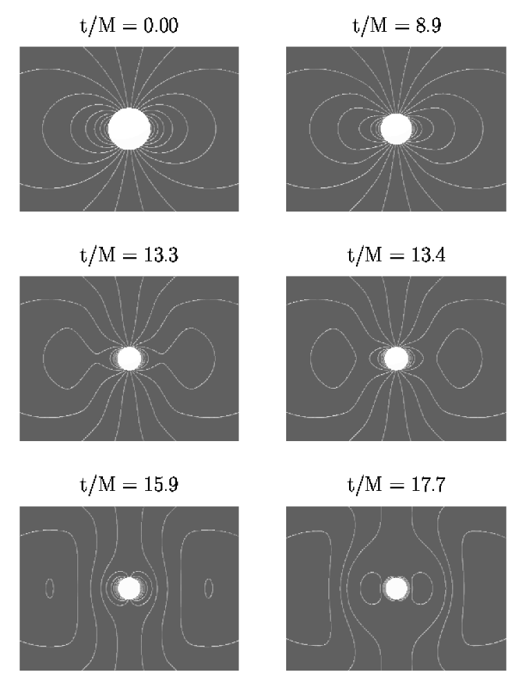
Figure 1: Snapshots of the exterior dipole magnetic field lines at select Schwarzschild time slices for a star which collapses from rest at an initial areal radius $R_{s}=4M$. Points are plotted in a meridional plane using areal radii. The light shaded sphere covers the matter interior. The initial growth of the longitudinal field due to flux freezing in the interior is ultimately followed by a outward burst of transverse electromagnetic radiation as the star approaches the black horizon at $r_{s}=2M$. Soon after the last snapshot at $t=17.7M$ the quality of the numerical integration deteriorates in this gauge. See text for details.

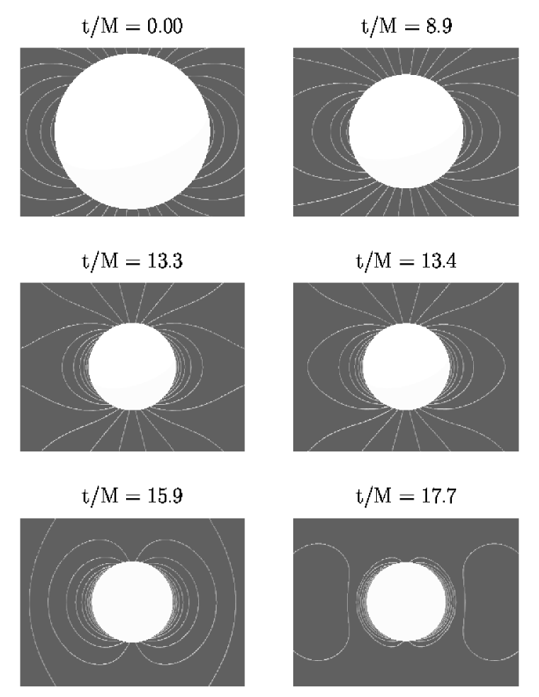
Figure 2: Blow-up of the same collapse depicted in Figure 1. Note how in this gauge the exterior field lines which are linked to the interior are crushed tangentially toward the surface as it approaches the horizon. Field lines which pinch off and become disjoint from the interior propagate outward as a dipole electromagnetic wave.

In Schwarzschild time slicing and isotropic coordinates, the exterior metric takes the form (5-4) with the lapse $\alpha$ given by

$$\alpha=\frac{1-M/(2r)}{1+M/(2r)},$$ (7-4)

the conformal factor $A$ given by

$$A=\left(1+\frac{M}{2r}\right)^{2},$$ (7-5)

and with the shift $\beta$ vanishing identically,

$$\beta=0.$$ (7-6)

In the above, the isotropic radius $r$ is related to the areal radius $r_{s}$ by

$$r_{s}=r\left(1+\frac{M}{2r}\right)^{2}$$ (7-7)

and

$$r=\frac{1}{2}\left(r_{s}-M+\left(r_{s}(r_{s}-2M)\right)^{1/2}\right).$$ (7-8)

The above quantities appear in the evolution equations (5-13) for $e$ and (5-14) $a$.

Analytic expressions for the areal radius $R_{s}$ of the stellar surface as a function of proper time $\tau$ have been given in Section 3 in terms of the parameter $\eta$. The isotropic radius can be found by substituting the areal radius into (7-8). The Schwarzschild coordinate time $t$ can also be found in terms of $\eta$ according to

$$t = 2M\ln\left(\frac{(R_{s}(0)/(2M)-1)^{1/2}+\tan(\eta/2)}{(R_{s}(0)/(2M)-1)^{1/2}-\tan(\eta/2)}\right)$$ (7-9)

$$+2M\left(\frac{R_{s}(0)}{2M}-1\right)^{1/2}\left(\eta+\frac{R_{s}(0)}{4M}(\eta+\sin\eta)\right)$$

(see, e.g. Misner, Thorne & Wheeler 1973, eqn. 32.10b). Note that we have $t/M\rightarrow\infty$ as the stellar surface approaches the event horizon, $R_{s}\rightarrow 2M$.

The velocity $v$ of the surface with respect to a normal observer is

$$v=\left(\frac{2M/R_{s}-2M/R_{s}(0)}{1-2M/R_{s}(0)}\right)^{1/2}.$$ (7-10)

This quantity enters the inner boundary condition for $e$, equation (5-30).

We have solved equations (5-13) and (5-14) in Schwarzschild slicing with an implicit finite differencing scheme (see Appendix B). We regrid after each timestep so that the stellar surface is always located half-way between the two first grid-points (which makes the implementation of the boundary conditions (5-29) and (5-30) particularly simple). The advantage of implicit schemes is that no Courant condition has to be satisfied to maintain stability of the numerical integration. Because of the linearity of Maxwell’s equations the initial field strength $B_{0}$ is arbitrary (provided it is dynamically unimportant) and can, without loss of generality, be chosen to be unity.

Figure 3: Electromagnetic energy conservation in Schwarzschild time slicing. The outer boundary is located at $R_{\rm out}=100M$, the exterior of the star is covered with 5000 gridpoints, and the Courant factor is unity. The solid line denotes the total energy $E$, which should be conserved (see equation  (A8)). The dotted line is the energy ${\mathcal{E}}(t)$ contained between the radii $r_{1}=1.01R_{s}(0)=4.04M$ and $r_{2}=80M$; the short dashed line is the integrated flux across $r_{1}$, ${\mathcal{J}}(r_{1})$, and the long dashed line is the integrated flux across $r_{2}$, ${\mathcal{J}}(r_{2})$. All energies are normalized to the initial energy $E_{0}$. Note that the quality of the numerical integration starts to deteriorate at about $t\sim 20M$, when the stellar surface and the ingoing electromagnetic waves approach the event horizon at $r_{s}=2M$.

In Figures 1 and 2 we show numerical results for a star collapsing from rest from an initial radius of $R_{s}(0)=4M$. In these snapshots we show the collapsing star together with exterior magnetic field lines. In axisymmetry, these field lines coincide with contours of constant $A_{\phi}$ (Zhang 1989), which enables us to draw them easily. At $t=0$ all field lines are attached to fluid interior and emerge from the stellar surface. At later times, as the surface approaches the event horizon, field lines that emerge from the surface are crushed against the star and become increasingly tangential (Anderson & Cohen 1970). At larger separations, field lines detach from the star during the collapse. In the radiation zone, these disjoint lines propagate outwards with the speed of light. Thus, early on, we find that the exterior longitudinal $B$ field evolves quasi-statically to match the growth of the frozen-in interior field (see equation (4-20)), while the exterior $E$ field remains small. At late times, the exterior longitudinal fields are radiated away and the dominant $B$ and $E$ fields become outgoing, decaying, transverse electromagnetic waves.

To calibrate the accuracy of the numerical integration we check the global conservation of magnetic energy as outlined in Appendix A. We show results of this energy conservation test in Figure 3. Clearly, the accuracy deteriorates soon after the surface of the star approaches the event horizon at around $t\sim 20M$. This effect is not surprising. The vanishing of the lapse (7-4) on the horizon causes the local light cone to “pinch off” and the (coordinate) speed of light to go to zero. As a consequence, incoming radiation piles up in front of the horizon and develops smaller and smaller spatial structures, which ultimately become smaller than any fixed grid resolution (cf. Rezzolla et at. 1998).

It is evident that Schwarzschild coordinates are not suitable for calculating the late-time radiation as measured by a distant observer, and, hence, for determining the late-time electromagnetic field decay rate. This observation motivates using a coordinate system that is regular on the event horizon and extends smoothly into the black hole interior.

7.3 Maximal Slicing: Interior and Exterior Solution

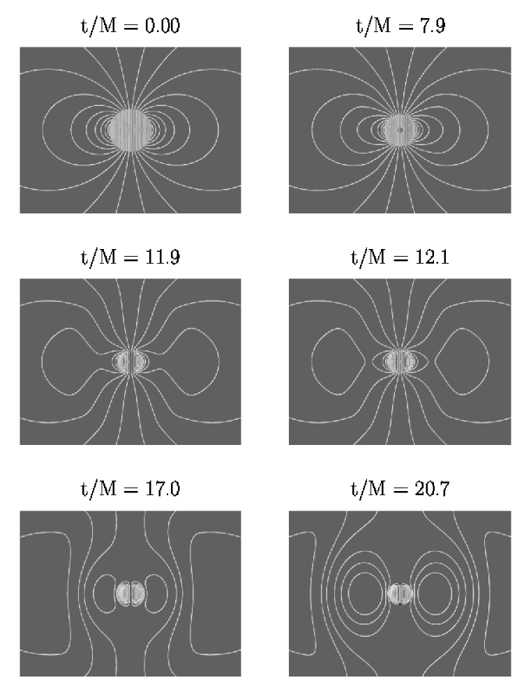
Figure 4: Snapshots of the interior and exterior magnetic field lines at select maximal time slices for the same collapse depicted in Figure 1. The star again collapses from rest at an initial areal radius $R_{s}(0)=4M$. Points are plotted in a meridional plane using areal radii. The light shaded sphere covers the matter interior; the black shaded sphere covers the region inside the event horizon. Soon after the last snapshot at $t=20.7$ grid stretching causes the quality of the numerical integration to deteriorate in this gauge. See text for details.

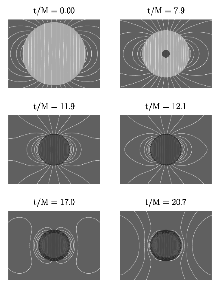
Figure 5: Blow-up of the same collapse depicted in Figure 4. Note how in this gauge the stellar surface approaches a limit surface at $r_{s}\approx 1.5M$ at late times. The horizon grows to its final value $r_{s}=2M$ once all the matter crosses inside this radius.

We now follow the same collapse but adopt maximal time slicing and isotropic (minimal shear) spatial coordinates. This coordinate system extends regularly into the black hole. Maximal slicing is imposed by requiring the trace of the extrinsic curvature to vanish at all times:

$$K=0=\frac{dK}{dt}.$$ (7-11)

Taking the trace of equation (I.2.8) then yields an elliptic equation for $\alpha$, which in general has to be solved numerically. Maximal slices of Oppenheimer-Snyder spacetime in isotropic coordinates may be determined by solving ordinary differential equations. Solutions are presented in Petrich, Shapiro & Teukolsky (1985) and provide $\alpha$, $\beta$ and $A$, which we substitute in equations (5-13) and (5-14) for the evolution of $e$ and $a$. These coordinates cover both the interior and the exterior of the star, so that we can map out the interior as well as the exterior field on these slices.

The Lorentz factor between a normal observer and a comoving observer at the stellar surface $\gamma=-u_{a}n^{a}$ can be computed from the numerical solution presented in Petrich, Shapiro & Teukolsky (1985) (i.e., $\gamma=1/(1-T^{2})$ and $v=|T|$, where $T$ is given by equation (6.11) of that paper). This is the velocity that is needed in the boundary condition (5-30).

We numerically solve equations (5-13) and (5-14) on maximal slices using implicit finite difference equations that are identical in form to those used on Schwarzschild slices (see Appendix B).

In Figures 4 and 5 we show snapshots of the collapse in maximal slicing. Unlike Schwarzschild slices and the Kerr-Schild slices below, maximal slicing also covers the matter interior, which allows us to trace the interior magnetic field lines as well as locate the apparent and event horizons in these plots. We can also identify the limit surface at $R_{s}\approx 1.5M$ which the matter surface approaches at late times (Petrich, Shapiro & Teukolsky 1985). Note that in the interior, a field line must connect the same Lagrangian fluid element at all times to satisfy the “frozen-in” requirement of MHD. This criterion provides a check on our field line tracer. For comoving observers in the interior, the electric field vanishes, but as viewed by a normal observer in maximal slicing the electric field is non-vanishing in general (see Section 5.2.1 for the transformation).

In maximal slicing the metric is not static, so that we cannot simply apply the electromagnetic energy conservation check developed in Appendix A.

Maximal slicing has some very desirable properties, but at late times grid stretching effects make the computation even of the background models increasingly difficult (Shapiro & Teukolsky 1986). We terminated the calculation shortly after $t=20M$.

7.4 Kerr-Schild Slicing: Black Hole Excision

The problems of maximal slicing can be avoided by using Kerr-Schild (or ingoing Eddington-Finkelstein) coordinates, which are analytic but smoothly extend across the horizon. This slicing is not “singularity avoiding”, so that it requires that the interior of a black hole be excised from the numerical grid. Adopting horizon-penetrating coordinate systems together with black hole excision is currently the most promising approach to dynamical simulations of black holes. In this calculation we apply this approach to the collapse of a magnetized star. Since the metric in Kerr-Schild coordinates (equation (7-12) below) takes a form that is different from (5-4), several parts of the above calculations, including the form of Maxwell’s equations, boundary conditions and initial data, have to be modified.

7.4.1 Kerr-Schild coordinates

In Kerr-Schild coordinates, the metric takes the form

$$ds^{2}=-(1-\frac{2M}{r_{s}})dt^{2}+\frac{4M}{r_{s}}dtdr_{s}+(1+\frac{2M}{r_{s}})dr_{s}^{2}+r_{s}^{2}d\Omega^{2},$$ (7-12)

where $r_{s}$ is the Schwarzschild (or areal) radius. From the metric we can identify the lapse as

$$\alpha=\left(\frac{r_{s}}{r_{s}+2M}\right)^{1/2},$$ (7-13)

the radial shift as

$$\beta=\frac{2M}{r_{s}+2M},$$ (7-14)

and the diagonal components of the spatial metric $\gamma_{ij}$ as

$$\gamma_{r_{s}r_{s}}=1+\frac{2M}{r_{s}}$$ (7-15)

and

$$\gamma_{\theta\theta}=\frac{1}{\sin^{2}\theta}\gamma_{\phi\phi}=r_{s}^{2}$$ (7-16)

(see, e.g., Lehner et al. 2000). The extrinsic curvature can then be computed from equation (I.2.9), which yields

$$K_{r_{s}r_{s}}=-\frac{2M}{r_{s}^{3}}(r_{s}+M)\alpha$$ (7-17)

and

$$K_{\theta\theta}=\frac{1}{\sin^{2}\theta}K_{\phi\phi}=2M\alpha.$$ (7-18)

The trace of the extrinsic curvature is

$$K=K^{i}_{~{}i}=\frac{2M}{r_{s}^{2}}\,\frac{1+3M/r_{s}}{(1+2M/r_{s})^{3/2}}=\frac{2M\alpha}{r_{s}^{2}}\,\frac{r_{s}+3M}{r_{s}+2M}.$$ (7-19)

7.4.2 Radial geodesics in Kerr-Schild coordinates

Figure 6: Electromagnetic energy conservation in Kerr-Schild time slicing. The outer boundary is located at $R_{\rm out}=100M$, the exterior of the star is covered with 5000 gridpoints, and the Courant factor is 0.5. The solid line denotes the total energy $E$, which should be conserved (see equation  (A8)). The dotted line is the energy ${\mathcal{E}}(t)$ contained between the radii $r_{1}=1.01R_{s}(0)=4.04M$ and $r_{2}=80M$; the short dashed line is the integrated flux across $r_{1}$, ${\mathcal{J}}(r_{1})$, and the long dashed line is the integrated flux across $r_{2}$, ${\mathcal{J}}(r_{2})$. Note that approximately 80% of the energy enters the black hole, while only 20% is radiated away to infinity.

The surface of the collapsing star follows a radial geodesic, which can be determined as follows. The areal radius as a function of proper time has to satisfy the same equations,

$$\begin{array}[]{rcl}R_{s}&=&\displaystyle\frac{R_{s}(0)}{2}(1+\cos\eta)\\ \tau&=&\displaystyle\left(\frac{R_{s}^{3}(0)}{8M}\right)^{1/2}(\eta+\sin\eta)\end{array}$$ (7-20)

as before (see Section 3), since both quantities are gauge invariant parameters. Here $R_{s}(0)$ is the initial Schwarzschild radius at which the surface is momentarily at rest. An equation for the Kerr-Schild coordinate time $t$ can be derived from the conservation of $p_{t}$

$$p_{t}=g_{tt}p^{t}+g_{tr_{s}}p^{r_{s}}=\mbox{const}\equiv-E,$$ (7-21)

or

$$\left(1-\frac{2M}{r_{s}}\right)\frac{dt}{d\tau}-\frac{2M}{r_{s}}\frac{dr_{s}}{d\tau}=\tilde{E}.$$ (7-22)

Combining this equation with the normalization condition for the four-velocity, $u_{a}u^{a}=-1$, yields

$$\frac{dr_{s}}{d\tau}=-\left(\tilde{E}^{2}-1+\frac{2M}{r_{s}}\right)^{1/2}.$$ (7-23)

Evaluating this result for the surface at $\tau=0$, when $dR_{s}/d\tau=0$, determines the energy

$$\tilde{E}=\left(1-\frac{2M}{R_{s}(0)}\right)^{1/2}.$$ (7-24)

Inserting the last two equations into (7-22) then yields

$$\frac{dt}{d\tau}=\frac{(1-2M/R_{s}(0))^{1/2}}{1-2M/R_{s}}-\frac{2M}{R_{s}}\,\frac{(2M/R_{s}-2M/R_{s}(0))^{1/2}}{1-2M/R_{s}}.$$ (7-25)

Interestingly, this equation can be integrated analytically to yield

$$t=2M\left(\frac{R_{s}(0)}{2M}-1\right)^{1/2}\left(\eta+\frac{R_{s}(0)}{4M}(\eta+\sin\eta)\right)$$ (7-26)

$$+2M\ln\left(\frac{1+\frac{R_{s}}{2M}-\frac{2R_{s}}{R_{s}(0)}+2\sqrt{(\frac{R_{s}}{2M}-\frac{R_{s}}{R_{s}(0)})(1-\frac{R_{s}}{R_{s}(0)})}}{\frac{R_{s}(0)}{2M}-1}\right)$$

The coordinate time $t_{f}$ for infall from $r_{s}=R_{s}(0)>2M$ to the singularity at $r_{s}=0$ is therefore

$$t_{f}=2\pi M\left(1+\frac{R_{s}(0)}{4M}\right)\left(\frac{R_{s}(0)}{2M}-1\right)^{1/2}-2M\ln\left(\frac{R_{s}(0)}{2M}-1\right).$$ (7-27)

This time is evidently finite, which reflects the fact that Kerr-Schild coordinates are horizon penetrating. This also demonstrates the necessity of excising the black hole interior, since otherwise the central singularity would be encountered after $t=t_{f}$.

The Lorentz factor corresponding to a boost from an observer comoving with the stellar surface to a local normal observer can be found from

$$\gamma=-n_{a}u^{a}=\alpha u^{t}=\left(1-\frac{4M^{2}}{R_{s}^{2}}\right)^{-1/2}.$$ (7-28)

The relative velocity $v$ of the normal observer as measured by a comoving observer at the surface is then given by

$$v=-\frac{2M}{R_{s}}.$$ (7-29)

A minus sign appears in equation (7-29) because the shift drives the radial velocity of normal observer inward more rapidly than the surface.

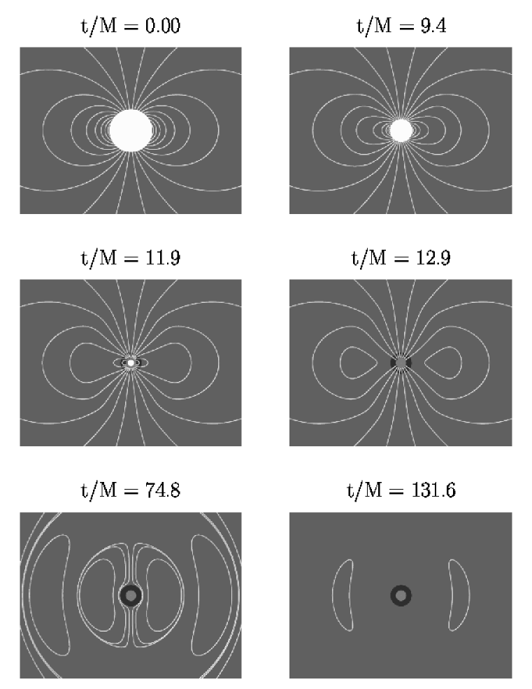
Figure 7: Snapshots of the exterior magnetic field lines at select Kerr-Schild time slices for the same collapse depicted in Figure 1. The star again collapses from rest at an initial areal radius $R_{s}(0)=4M$. Points are plotted in a meridional plane using areal radii. The white shaded sphere covers the matter interior; the black shaded area covers the region inside the event horizon; the grey shaded area covers the region inside $r_{s}=M$ excised from the numerical grid once the matter passes inside. In this gauge, using excision, we are able to integrate reliably to arbitrary late times. See text for details.

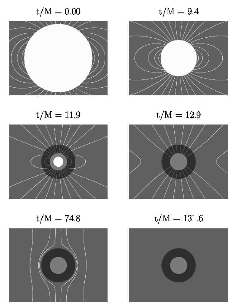
Figure 8: Blow-up of the same collapse depicted in Figure 7. By the end of the integration, all exterior electromagnetic fields in the vicinity of the black hole have been captured or radiated away.

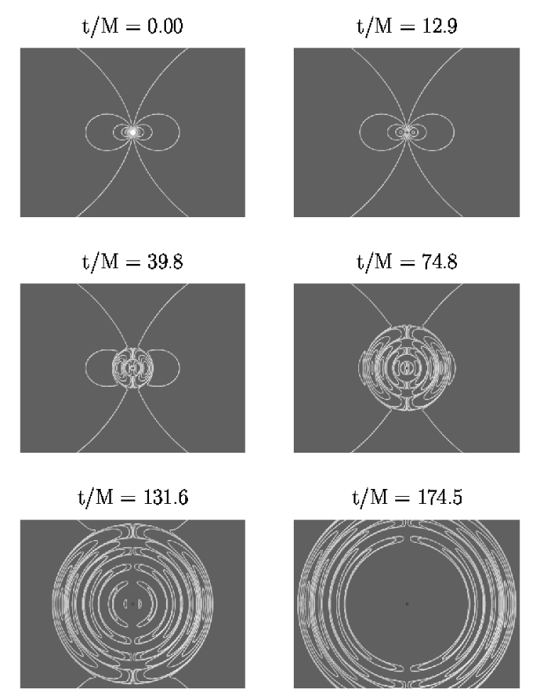
Figure 9: Far-zone view of the same same collapse depicted in Figures 7 and 8, but now extending to very late times. Note the transformation of the dipole magnetic field from a quasi-static longitudinal to a transverse electromagnetic wave.

7.4.3 Exterior initial data in Kerr-Schild coordinates

Given the boost parameters $\gamma$ and $v$, we can transform the magnetic dipole initial data of Section 6.2 into Kerr-Schild coordinates. Applying the transformation rules (5-15) we find

$$\begin{array}[]{rcl}B^{\hat{r}}_{\rm KS}&=&B^{\hat{r}}_{\rm WS}\\ B^{\hat{\theta}}_{\rm KS}&=&\gamma B^{\hat{\theta}}_{\rm WS}\\ B^{\hat{\phi}}_{\rm KS}&=&0\\ E^{\hat{r}}_{\rm KS}&=&E^{\hat{r}}_{\rm WS}=0\\ E^{\hat{\theta}}_{\rm KS}&=&\gamma(E^{\hat{\theta}}_{\rm WS}-vB^{\hat{\phi}}_{\rm WS})=0\\ E^{\hat{\phi}}_{\rm KS}&=&\gamma(E^{\hat{\phi}}_{\rm WS}+vB^{\hat{\theta}}_{\rm WS})=\gamma vB^{\hat{\theta}}_{\rm WS}.\end{array}$$ (7-30)

Here the subscript KS refers to Kerr-Schild data, and WS to the Wasserman-Shapiro exterior magnetic dipole solution presented in Section 6.2. We note that even at $t=0$ the electric field is non-vanishing as seen by a normal observer in Kerr-Schild coordinates, since a normal observer is moving with respect to a static observer.

7.4.4 Maxwell’s equations in Kerr-Schild coordinates

Figure 10: The absolute value of the radial magnetic field $|B^{\hat{r}}|$ at $r=20M$ as a function of time. For this simulation, the outer boundary was placed at $2000M$, the numerical grid consisted of 6000 radial gridpoints, and the Courant factor was 0.5. The dashed line is a power law $t^{-4}$, which approximates the late-time fall-off extremely well.

Figure 11: Same as Fig. 10, except for $|B^{\hat{\theta}}|$.

Figure 12: Same as Fig. 10, except for $|E^{\hat{\phi}}|$.

In Section 5.1 we evaluated Maxwell’s equations (5-1) and (5-2) for a metric of the form (5-4). Since the Kerr-Schild metric (7-12) has a slightly different form, we have to re-evaluate Maxwell’s equations.

Our derivation closely follows that of Section 5.1. We insert the metric coefficients of Section 7.4.1 into equations (5-1) and (5-2), choose the Coulomb gauge condition by setting $\Phi=0$, ensure axisymmetric fields by assuming that $A_{\phi}=A_{\phi}(t,r,\theta)$ and $E^{\phi}=E^{\phi}(t,r,\theta)$ are the only non-vanishing components, and finally use the expansions (5-7) and (5-11). The resulting equations for $e$ and $a$ are

$$\partial_{t}e=\alpha\left(\alpha^{2}a_{,r_{s}}\right)_{,r_{s}}-\alpha\,\frac{l(l+1)}{r_{s}^{2}}\,a+\alpha Ke+\beta r_{s}^{2}\left(\frac{e}{r_{s}^{2}}\right)_{,r_{s}}$$ (7-31)

and

$$\partial_{t}a=\alpha e+\beta a_{,r_{s}},$$ (7-32)

where the metric coefficients $\alpha$ and $\beta$ and the trace of the extrinsic curvature $K$ are given in Section 7.4.1.

In terms of $e$ and $a$, the components of the electric and magnetic fields are given by

$$E^{\hat{\phi}} = \frac{\sin\theta}{r_{s}}\,e$$ (7-33)

$$B^{\hat{r}} = -\frac{2\cos\theta}{r_{s}^{2}}\,a$$ (7-34)

$$B^{\hat{\theta}} = \frac{\sin\theta}{(1+2M/r_{s})^{1/2}r_{s}}\,a_{,r_{s}}.$$ (7-35)

7.4.5 Boundary Conditions

For the early part of the evolution, the inner boundary conditions result from junction conditions on the electromagnetic fields at the stellar surface. The derivation of these conditions follows that of Section 5.2.1 and results in

$$a=-\frac{r_{s}^{2}B_{\hat{r}}^{(in)}}{2\cos\theta}$$ (7-36)

and

$$e=\frac{v}{(1+2M/r_{s})^{1/2}}\,a_{,r_{s}}.$$ (7-37)

Once the stellar surface has passed through some radius $R_{\rm ex}<2M$ inside the horizon, we switch from the junction condition on the stellar surface to an excision boundary condition at $R_{\rm ex}$. We typically set $R_{\rm ex}=M$, but the results are insensitive to the choice provided $R_{\rm ex}$ is well inside the horizon at $2M$. Once we have switched to an excision boundary condition, we fix the numerical grid so that $R_{\rm ex}$ is located half-way between the first two gridpoints.

We have experimented with a number of different excision boundary conditions, but found, as expected, that the exact implementation had hardly any effect on the results in the exterior of the black hole, as long as $R_{\rm ex}$ is far enough inside the event horizon. Following a similar approach by Alcubierre & Brügmann (2001) for dynamical black hole simulations, we settled on simply copying the values of $e$ and $a$ from the second gridpoint to the first at every timestep, which is equivalent to imposing

$$e_{,r_{s}}=a_{,r_{s}}=0$$ (7-38)

(see equations (B13) and (B14)).

7.4.6 Numerical results

We have implemented the evolution equations (7-31) and (7-32) using both implicit and explicit finite difference methods (see Appendix B for the finite difference equations). The results presented here were obtained with the explicit scheme.

Since the Kerr-Schild metric (7-12) is independent of time, we can calibrate the performance of the code with the same global electromagnetic energy conservation test as we did in Schwarzschild coordinates (Section 7.2). The necessary expressions can be found in Appendix A. We show results for the energy conservation check in Figure 6. It is quite obvious that this integration works much better than that in Schwarzschild coordinates (cf. Figure 3), due to regularity across the horizon. We can follow the electromagnetic fields to arbitrary late times, and can track the late-time behavior reliably.

Figure 6 also shows that about 80% of the energy contained in the initial magnetic field is absorbed by the black hole, while about 20% of the radiation is emitted in an electromagnetic wavepacket.

In Figures 7 through 9 we show snapshots of magnetic field lines for a star collapsing from $R_{s}(0)=4M$ as viewed in three different regions. It can be seen very clearly how the collapse of the magnetized star emits a pulse of electromagnetic radiation, which travels to infinity at the speed of light. Similar behavior is seen in plots of the electric field at late times.

We can now evaluate the late-time fall-off of the electromagnetic fields. In Figures 10 through 12 we show the values of $|B^{\hat{r}}|$, $|B^{\hat{\theta}}|$ and $|E^{\hat{\phi}}|$ at $r=20M$ as a function of time. As expected, the fields are nearly constant up to $t=20M$. Once the collapse gets underway, the exterior longitudinal field starts to evolve to match the increasing interior frozen-in field. Soon after $t=20M$, the first electromagnetic pulse induced by the collapse passes the observer at $r=20M$. Sign changes in the field appear as down-ward spikes in the plots. After $t\sim 100M$, the exterior fields are predominantly characterized by a decaying dipole with a power-law fall-off with time. In Figures 10 through 12 we have plotted the power-laws curves varying like $t^{-4}$ to which the fields approach for late times. This finding for the exterior fields agrees with the general results of Price (1972a,b; cf. Thorne, 1971) who showed that multipole electromagnetic fields scattering off a static Schwarzschild black hole should decay as $t^{-(2l+2)}$.

Measurement of the wavelength of the late-time outgoing electromagnetic waves provides further verification of our numerical integrations. We find that the wavelength satisfies $\lambda\approx 24.7M$. This is the value of a quasi-normal mode for electromagnetic dipole radiation scattering off a static Schwarzschild black hole (Ferrari & Mashhoon 1984). This finding shows that the late-time radiation is ringing radiation that has a frequency determined by the mass of the hole and is independent of the initial electromagnetic field profile.

8 Summary

We have solved for the evolution in general relativity of the electromagnetic field of a magnetic star that collapses from rest to a Schwarzschild black hole. We adopted a “dynamical Cowling” model by which the matter and gravitational field are prescribed by the Oppenheimer-Snyder solution for spherical collapse. Starting from Maxwell’s equations in $3+1$ form, we solved for the magnetic and electric fields both in the vacuum exterior and the stellar interior. We assumed that the initial star was threaded by a dipole magnetic field and that the interior behaves as an MHD fluid. We showed how the electromagnetic junction conditions could be applied at the stellar surface in order that the fields in the MHD interior, which were determined analytically, could be matched to the fields in the vacuum exterior. The exterior fields were evolved numerically.

To gain experience with solving Maxwell’s equations numerically in a dynamical spacetime containing both matter and a black hole, we solved the above problem in three different coordinate gauges: Schwarzschild, maximal and Kerr-Schild. While the first two coordinate systems have singularity avoiding properties, they both lead to growing numerical inaccuracies in the exterior as the surface approaches the horizon (in the case of Schwarzschild time slicing) or a limit surface inside the horizon (in the case of maximal slicing) at late times. Kerr-Schild slicing is horizon penetrating and does not suffer from grid stretching; accordingly this slicing enables us to apply excision boundary conditions once the star collapses inside the horizon. Adopting Kerr-Schild slicing coordinates with black hole excision allowed us to integrate Maxwell’s equations to arbitrary late times. We followed the transition in the exterior of a quasi-static, longitudinal magnetic field, which evolved during the collapse in to match the growing frozen-in interior field, to a transverse electromagnetic wave. By the end of the simulation, the electromagnetic field energy in the near zone outside the black hole had either been captured by the hole or radiated away to large distances, in accord with the “no-hair theorem”. At late times we recovered the expected power-law decay of the dipole fields with time, as well as the expected wavelength of the ringdown radiation.

There exist a number of very important astrophysical problems which require the solution of the coupled Maxwell-Einstein-MHD equations in a strong, dynamical gravitational field. For example, learning the outcome of rotating stellar core or supermassive star collapse, the mechanism for gamma-ray bursts, and/or the fate of the remnant of a binary neutron star merger may all require solving this coupled system of equations. The solution we have presented for our simple collapse scenario should serve as a preliminary guide to the design and testing of more sophisticated codes capable of handling these more complicated scenarios.

Appendix A Global Electromagnetic Energy Conservation

A.1 General Discussion

The conservation of energy can be verified very easily if the exterior metric is independent of time, so that

$${\bf\xi}=\frac{\partial}{\partial t}$$ (A1)

is a Killing vector. In that case,

$$J_{\mu}\equiv T_{\mu\nu}\xi^{\nu}$$ (A2)

is a conserved current and satisfies

$$\oint_{\partial V}J^{\alpha}d^{3}\Sigma_{\alpha}=0,$$ (A3)

where ${\partial V}$ denotes the 3-surface enclosing the 4-volume $V$. If the volume $V$ is confined by the radii $r_{1}$ and $r_{2}$ and the times $t_{1}$ and $t_{2}$, the conservation law can be written as

$$\displaystyle\left.\int_{r=r_{1}}^{r_{2}}\int_{\theta=0}^{\pi}\int_{\phi=0}^{2\pi}J^{0}\sqrt{-g}drd\theta d\phi\right|_{t_{1}}^{t_{2}}$$ (A4)

$$\displaystyle~{}~{}~{}=-\left.\int_{t=t_{1}}^{t_{2}}\int_{\theta=0}^{\pi}\int_{\phi=0}^{2\pi}J^{r}\sqrt{-g}dtd\theta d\phi\right|_{r_{1}}^{r_{2}}$$ .

Defining the energy contained between $r_{1}$ and $r_{2}$ at time $t$ as

$${\mathcal{E}}(t)\equiv\int_{r=r_{1}}^{r_{2}}\int_{\theta=0}^{\pi}\int_{\phi=0}^{2\pi}J^{0}\sqrt{-g}drd\theta d\phi$$ (A5)

and the integrated flux across the radius $r$ as

$${\mathcal{J}}(r)\equiv\int_{t=t_{1}}^{t_{2}}\int_{\theta=0}^{\pi}\int_{\phi=0}^{2\pi}J^{r}\sqrt{-g}dtd\theta d\phi$$ (A6)

the conservation law can be rewritten as

$${\mathcal{E}}(t_{2})-{\mathcal{E}}(t_{1})={\mathcal{J}}(r_{2})-{\mathcal{J}}(r_{1}).$$ (A7)

The meaning of this statement is quite evident: the difference in the energy contained between $r_{1}$ and $r_{2}$ at two different times has to equal the net energy flux entering the region, integrated over the time interval. An alternative way of writing the conservation law is

$$E/E_{0}=\left({\mathcal{E}}(t_{2})-{\mathcal{J}}(r_{2})+{\mathcal{J}}(r_{1})\right)/E_{0}=1,$$ (A8)

where $E_{0}={\mathcal{E}}(t_{1})$ is the initial energy between $r_{1}$ and $r_{2}$. We use equation (A8) in plotting our results in the text.

Since the exterior metric is independent of time in both Schwarzschild coordinates (Section 7.2) and Kerr-Schild coordinates (Section 7.4), energy conservation can be verified quite easily in both of those coordinate systems. To do so, the energy (A5) and the flux (A6) have to be expressed in terms of the relevant metric quantities, which we do separately in the two following Sections. A similar analysis was used in Appendix A of Pavlidou, Tassis, Baumgarte & Shapiro (2000) for the energy conservation of a scalar field in the static spacetime of a spherical, equilibrium star.

A.2 Schwarzschild Slicing

In isotropic Schwarzschild coordinates the metric takes the form (5-4) with $\alpha$, $A$ and $\beta$ given by (7-4), (7-5) and (7-6). The determinant of the metric is

$$\sqrt{-g}=\alpha A^{3}r^{2}\sin\theta,$$ (A9)

and the fluxes $J^{0}$ and $J^{r}$ in (A5) and (A6) can be expressed as

$$J^{0}=T^{0}_{~{}0}=T^{\hat{0}}_{~{}\hat{0}}=-T^{\hat{0}\hat{0}}=-\frac{1}{8\pi}({\bf E}^{2}+{\bf B}^{2})$$ (A10)

and

$$J^{r}=T^{r}_{~{}0}=\frac{\alpha}{A}T^{\hat{r}}_{~{}\hat{0}}=-\frac{\alpha}{A}T^{\hat{r}\hat{0}}=-\frac{\alpha}{4\pi A}({\bf E\times B})^{\hat{r}}.$$ (A11)

Here we have used the results of Section 7 of Paper I to evaluate the source terms. The fields ${\bf E}$ and ${\bf B}$ can now be expressed in terms of $e$ and $a$ using equations (5-26), (5-27) and (5-28) for an $l=1$ dipole field. The angular integrals in equation (A5) and (A6) can be carried out analytically, yielding

$${\mathcal{E}}(t)=\frac{1}{2}\int_{r_{1}}^{r_{2}}dr(\alpha A^{2})\left(\frac{2}{3}A^{3}e^{2}+\frac{4}{3}\,\frac{a^{2}}{A^{3}r^{2}}+\frac{2}{3}\,\frac{(a_{,r})^{2}}{A^{3}}\right)$$ (A12)

and

$${\mathcal{J}}(t)=\frac{2}{3}\alpha^{2}A\int_{t_{1}}^{t_{2}}dt(a_{,r}e).$$ (A13)

These expressions can now be inserted into equation (A8) to verify energy conservation in Schwarzschild coordinates.

A.3 Kerr-Schild coordinates

In Kerr-Schild coordinates, the determinant of the metric is

$$\sqrt{-g}=r_{s}^{2}\sin\theta.$$ (A14)

The fluxes $J^{0}$ and $J^{r_{s}}$ in (A5) and (A6) are easiest evaluated by using the form (I.7.8) for the electromagnetic stress-energy tensor $T^{ab}$. We then find

$$4\pi J^{0}=4\pi T^{0}_{~{}0}=\frac{1}{2}n^{0}n_{0}(E_{i}E^{i}+B_{i}B^{i})+n^{0}\epsilon_{0lm}E^{l}B^{m}.$$ (A15)

Here $\epsilon_{0lm}=-\beta\epsilon_{lr_{s}m}$ (see (I.3.19)) and restricting the summations to the only non-vanishing components $E^{\hat{\phi}}$, $B^{\hat{r}}$ and $B^{\hat{\theta}}$ yields

$$4\pi J^{0}=-\frac{1}{2}({\bf E}^{2}+{\bf B}^{2})-\frac{1+2M/r_{s}}{1+r_{s}/{2M}}E^{\hat{\phi}}B^{\hat{\theta}}.$$ (A16)

The radial component can be evaluated in a similar way, which leads to

$$4\pi J^{r} = \frac{1}{1+r_{s}/(2M)}\left((E^{\hat{\phi}})^{2}+(B^{\hat{\theta}})^{2}\right)$$

$$+\left(\frac{1+2M/r_{s}}{(1+r_{s}/(2M))^{2}}+\frac{1}{1+2M/r_{s}}\right)E^{\hat{\phi}}B^{\hat{\theta}}.$$

Specializing to $l=1$ dipole fields, the angular integrals in equation (A5) and (A6) can again be carried out analytically, which yields

$${\mathcal{E}}(t) = \frac{1}{2}\int_{r_{1}}^{r_{2}}dr_{s}r_{s}^{2}\Big{(}\frac{2}{3}\frac{e^{2}}{r_{s}^{2}}+\frac{4}{3}\frac{a^{2}}{r_{s}^{4}}$$

$$+\frac{2}{3}\frac{(a_{,r_{s}})^{2}}{(1+2M/r_{s})r_{s}^{2}}+\frac{4}{3}\frac{ea_{,r_{s}}}{r_{s}^{2}}\,\frac{(1+2M/r_{s})^{1/2}}{1+r_{s}/(2M)}\Big{)}$$

and

$${\mathcal{J}}(t) = \frac{2}{3}\int_{t_{t}}^{t_{2}}dt\Big{\{}\frac{1}{1+r_{s}/(2M)}\Big{(}e^{2}+\frac{(a_{,r_{s}})^{2}}{1+2M/r_{s}}\Big{)}$$

$$+\Big{(}\frac{(1+2M/r_{s})^{1/2}}{(1+r_{s}/(2M))^{2}}+\frac{1}{(1+2M/r_{s})^{3/2}}\Big{)}ea_{,r_{s}}\Big{\}}$$

These expressions can be inserted into equation (A8) to verify energy conservation in Kerr-Schild coordinates.

Appendix B Finite-Difference Equations

To finite difference the coupled evolution equations (5-13) and (5-14) for Schwarzschild or maximal slicing (or (7-31) and (7-32) in the Kerr-Schild case) we introduce a uniform radial grid $r_{i},i=1,2,...,I$. We regrid the radial gridpoints after each timestep, using linear interpolation between the old gridpoints, so that the stellar surface $R_{s}$ is always half-way between the first two gridpoints at $(r_{1}+r_{2})/2$. In the Kerr-Schild simulations this is no longer necessary once the interior of the black hole has been excised and the inner boundary condition is imposed at a constant excision radius $R_{\rm ex}$. All variables are defined at the gridpoint $r_{i}$. Note that our numerical grid never extends to $r=0$. In the following we use $\Delta t=t^{n+1}-t^{n}$ and $\Delta r=r_{i+1}-r_{i}$.

B.1 Schwarzschild Coordinates and Maximal Slicing

For isotropic Schwarzschild coordinates (Section 7.2) and maximal slicing (Section 7.3) we adopt an implicit evolution scheme. It is convenient to use the abbreviations

$$B=\frac{\alpha}{A}$$ (B1)

and

$$C=A^{3}.$$ (B2)

Finite difference representations of equations (5-13) and (5-14) can then be written as

$$\frac{a^{n+1}_{i}-a^{n}_{i}}{\Delta t}=B^{n+1}_{i}C^{n+1}_{i}e^{n+1}_{i}+\beta^{n+1}_{i}\left(\frac{a^{n+1}_{i+i}-a^{n+1}_{i-1}}{2\Delta r}\right)$$ (B3)

and

$$\frac{e^{n+1}_{i}-e^{n}_{i}}{\Delta t}=\frac{1}{C^{n+1}_{i}}\,\frac{1}{(\Delta r)^{2}}$$ (B4)

$$\times\left(B^{n+1}_{i+1/2}(a^{n+1}_{i+1}-a^{n+1}_{i})-B^{n+1}_{i-1/2}(a^{n+1}_{i}-a^{n+1}_{i-1})\right)$$

$$-\frac{B^{n+1}_{i}}{C^{n+1}_{i}}\frac{l(l+1)}{r_{i}^{2}}a^{n+1}_{i}+\beta^{n}_{i}\frac{r_{i}^{2}}{2\Delta r}\left(\frac{e^{n}_{i+1}}{r_{i+1}^{2}}-\frac{e^{n}_{i-1}}{r_{i-1}^{2}}\right).$$

Here the midpoint values $B^{n+1}_{i+1/2}$ are computed as linear interpolations $(B^{n+1}_{i+1}+B^{n+1}_{i})/2$. Note also that we have finite-differenced the shift term implicitly in (B3), but explicitly in (B4).

The boundary condition (5-29) is implemented as

$$\frac{a^{n+1}_{1}+a^{n+1}_{2}}{2}=-(A^{n+1}_{3/2}r_{3/2})^{2}\frac{B}{2},$$ (B5)

where the interior field strength $B$ is given by equation (6-6). The outer boundary condition (5-32) is finite differenced as

$$\frac{a^{n+1}_{I}-a^{n}_{I}}{\Delta t}=-\frac{a^{n}_{I}-a^{n}_{I-1}}{\Delta r}-\frac{a^{n}_{I}}{r_{I}}$$ (B6)

Substituting the finite difference equation (B4) into (B3) and using equations (B5) and (B6) at the inner and outer boundaries yields a single tridiagonal matrix equation for $a^{n+1}_{i}$. For this approach to work we had to finite-difference the shift terms in (B4) explicitly, because these would have otherwise introduced $e^{n+1}_{i}$ terms into the equation for $a^{n+1}_{i}$. We invert the tridiagonal matrix at each time step to obtain the new values $a^{n+1}_{i}$. New values $e^{n+1}_{i}$ can then be found by using equation (B4) again together with the inner boundary condition (5-30)

$$\frac{e^{n+1}_{1}+e^{n+1}_{2}}{2}=\frac{v^{n+1}_{3/2}}{C^{n+1}_{3/2}}\,\frac{a^{n+1}_{2}-a^{n+1}_{1}}{\Delta r}$$ (B7)

and an outer boundary condition equivalent to (B6).

To choose the size for successive timesteps we set

$$\Delta t={\mathcal{C}}~{}{\rm min}\left(\Delta r\right),$$ (B8)

where we have introduced a Courant factor ${\mathcal{C}}$ in the above equation. Implicit differencing imposes no restrictions on ${\mathcal{C}}$, but accuracy usually requires the choice ${\mathcal{C}}\lesssim 1$.

B.2 Kerr-Schild Slicing

The evolution equations (7-31) and (7-32) in Kerr-Schild slicing can be finite differenced in a very similar fashion to those in Schwarzschild coordinates or maximal slicing.

In addition to an implicit scheme, we also implemented an iterative explicit scheme, in which case the finite difference equations are written as

$$\frac{a^{n+1}_{i}-a^{n}_{i}}{\Delta t}=\alpha^{n}_{i}e^{n}_{i}+\beta^{n}_{i}\left(\frac{a^{n}_{i+i}-a^{n}_{i-1}}{2\Delta r}\right)$$ (B9)

and

$$\frac{e^{n+1}_{i}-e^{n}_{i}}{\Delta t}=\frac{\alpha^{n}_{i}}{(\Delta r)^{2}}$$ (B10)

$$\times\left((\alpha^{n}_{i+1/2})^{2}(a^{n}_{i+1}-a^{n}_{i})-(\alpha^{n}_{i-1/2})^{2}(a^{n}_{i}-a^{n}_{i-1})\right)$$

$$-\alpha^{n}_{i}\frac{l(l+1)}{r_{i}^{2}}a^{n}_{i}+\alpha^{n}_{i}K^{n}_{i}e^{n}_{i}$$

$$+\beta^{n}_{i}\frac{r_{i}^{2}}{2\Delta r}\left(\frac{e^{n}_{i+1}}{r_{i+1}^{2}}-\frac{e^{n}_{i-1}}{r_{i-1}^{2}}\right).$$

Here the radius $r$ denotes an areal radius in this Section (denoted with $r_{s}$ in the rest of the paper). Prior to excision, the boundary conditions (7-36) and (7-37) can be finite-differenced as

$$\frac{a^{n+1}_{1}+a^{n+1}_{2}}{2}=-\frac{(r_{3/2})^{2}B}{2}$$ (B11)

and

$$\frac{e^{n+1}_{1}+e^{n+1}_{2}}{2}=\frac{v^{n+1}_{3/2}}{(1+2M/r_{3/2})^{1/2}}\,\frac{a^{n+1}_{2}-a^{n+1}_{1}}{\Delta r}$$ (B12)

Once the stellar radius is smaller than the excision radius $R_{\rm ex}$ we switch to the excision boundary conditions (7-38), which can be implemented as

$$a^{n+1}_{1} = a^{n+1}_{2}$$ (B13)

$$e^{n+1}_{1} = e^{n+1}_{2}$$ (B14)

The outer boundaries are identical to those for Schwarzschild coordinates and maximal slicing.

An iterative Crank-Nicholson scheme can be constructed in the following way (cf. Teukolsky 2000). In a predictor step, the above equations are solved for approximate new values $\tilde{a}^{n+1}_{i}$ and $\tilde{e}^{n+1}_{i}$. The average between these values and the old values ${a}^{n}_{i}$ and ${e}^{n}_{i}$ is then used on the right hand side to compute improved new values $\bar{a}^{n+1}_{i}$ and $\bar{e}^{n+1}_{i}$ in a first corrector step. These are again averaged with ${a}^{n}_{i}$ and ${e}^{n}_{i}$ and used on the right hand sides for the second and final corrector step, which yields the new values ${a}^{n+1}_{i}$ and ${e}^{n+1}_{i}$.

The Kerr-Schild results presented here were obtained with the above explicit scheme. However, we also implemented an implicit scheme very similar to that in Section B.1 and obtained very similar results. In particular, we found the interesting result that excision boundary conditions (7-38) can be used with an implicit scheme without encountering problems. Implemented as in Section B.1, the implicit scheme is first order in time (but could easily be made second order), while the above iterative scheme is second order in time, which resulted in more accurate results in late-time evolutions.