Investigations of Pointwise Ignition of Helium Deflagrations on Neutron Stars

Abstract

We look at the spreading of localized temperature perturbations in the accreted fuel layer of a non-rotating neutron star. The pressure at the base of the accreted fuel layer is large and the material is only partially degenerate. Any temperature perturbations and resulting pressure gradients will lead to enormous accelerations (both laterally and vertically) of the material in the fuel layer. If the burning of this fuel cannot proceed more rapidly than the spreading of this perturbation, then localized burning cannot take place, and it is likely that the ignition would have to proceed simultaneously throughout the envelope. We present some multidimensional simulations of the spreading of temperature perturbations in a helium atmosphere on a neutron star.

University of California Santa Cruz, Santa Cruz, CA, 95064

University of Chicago, Chicago, IL 60637

1. Introduction

We wish to investigate whether localized burning can occur in the accreted atmosphere of a neutron star. A summary of the observations of type I X-ray bursts is presented by Cumming (2002) in this proceedings. Fryxell & Woosley (1982) made some estimates of how fast a deflagration can travel through a fuel layer, considering multidimensional effects. We look to see whether it is possible to setup such a deflagration to begin with. Given a temperature perturbation at the base of the fuel layer, a pressure gradient will result, which will act to smooth out this initial perturbation. This gradient will drive velocities which will spread out the initial perturbation. We want to determine whether it is possible for nuclear burning to act on a timescale that is faster than this spreading timescale.

2. Nuclear Timescales

The nuclear rise time for a region of fuel is computed as

$$\tau_{\rm{nuc}}=\int_{T_{\rm{fuel}}}^{2T_{\rm{fuel}}}\frac{c_{p}\rm{d}T}{e_{\rm{nuc}}{\dot{X}}_{\rm{fuel}}}$$ (1)

If we cannot burn faster than the spreading time of a perturbation, then the burning will not be localized. Figure 1 shows the nuclear timescales for several different densities of pure helium as a function of temperature, using the 3-$\alpha$ reaction. We see that the fastest burning timescale is $\sim 0.08$s—-this is long compared to the dynamical timescales that we consider in the next section.

Figure 1.: Nuclear timescales vs temperature for 5 different densities (from top to bottom, $5\times 10^{5}\ \rm{g\ cm^{-3}}$, $7.1\times 10^{5}\ \rm{g\ cm^{-3}}$, $1\times 10^{6}\ \rm{g\ cm^{-3}}$, $1.4\times 10^{6}\ \rm{g\ cm^{-3}}$, and $2\times 10^{6}\ \rm{g\ cm^{-3}}$) for the 3-$\alpha$ reaction.

We want how long it takes for two regions of fuel (hot and cool) to show differences—we want to compare the rates of the burning

$$\Delta\tau_{\rm{nuc}}=\frac{1}{1/\tau_{\rm{hot}}-1/\tau_{\rm{cool}}}$$ (2)

Two regions of fuel that have nearly the same temperature will have very close nuclear rise times ($\tau_{\rm{hot}}\sim\tau_{\rm{cool}}$), so $\Delta\tau_{\rm{nuc}}$ will be large—it takes a long time to see any differences.

We can ignite locally if the time for the temperature perturbation to spread away is longer than $\Delta\tau_{\rm{nuc}}$. For each density, we need to find the initial conditions (if they exist) that result in a spreading time that is slower than this nuclear timescale.

3. Estimates of the Spreading Timescale

Any temperature gradient on the grid will produce a pressure gradient, that will lead to a lateral acceleration. The acceleration laterally through the atmosphere can be integrated to yield an estimate for the spreading velocity,

$$a_{x}=\frac{{\bf\nabla}P\cdot{\bf\hat{x}}}{\rho}\Longrightarrow v_{x}\approx c_{s}\left({\frac{\delta P}{P}}\right)^{1/2}$$ (3)

An initial 20% temperature perturbation is a $\sim 6\%$ pressure perturbation (at a density of $2\times 10^{6}\ \rm{g\ cm^{-3}}$), which leads to a velocity of $\sim 7\times 10^{7}\ \rm{cm\ s^{-1}}$. If our initial perturbation is 1000 cm across, this would spread in $\sim 15\ \mu s$. Note that $\delta P$ decreases as the material spreads, so this is the fastest case.

Rotation can have a stabilizing effect on the spreading of an initial perturbation (Spitkovsky, Levin, & Ushomirsky 2002). There is a scale (Rossby deformation length) at which the Coriolis force will balance a pressure gradient:

$$L=\sqrt{gH_{0}}/f$$ (4)

where f is the Coriolis force and $H_{0}$ is the scale height. Perturbations smaller than this scale will spread until they reach this length. For a 300 Hz rotation speed, this scale is about 10 km. This means that any temperature perturbation will spread out until it reaches 10 km. This allows us to define what we mean by non-rotation—the maximum size for $L$ is the circumference of the neutron star, so if the rotational frequency is less than $\sim 100\ \rm{Hz}$, then rotation will not matter. This is the regime that we are considering presently.

4. Initial Conditions

Figure 2.: Initial model in the maximally perturbed region, showing temperature and density. This model is in hydrostatic equilibrium (HSE) vertically. The temperature perturbation is placed at the fuel/ash interface ($1500\ \rm{cm}$). The density, temperature, and composition in the zone immediately below the interface are identical in all models, so the models have equal pressures at all heights lower than the interface.

The initial model we use to study the spreading of a perturbation through a neutron star atmosphere consists of a fuel and ash region, in HSE vertically, and in lateral pressure equilibrium in the ash region. It is impossible to put an initial model in HSE vertically and pressure equilibrium laterally if the temperatures at the bases differ.

The initial conditions are created by computing separate initial models for each column of zones on the grid. The fuel is pure ⁴He with a (possible) temperature perturbation at its base. The ash is pure ⁵⁶Ni and completely isothermal. The model is completely specified by the ash temperature ($T_{\rm{ash}}$), the temperature and density at the base of the fuel layer, and the height of the interface.

For the present simulations, we choose the density at the base of the fuel layer to be $2\times 10^{6}\ \rm{g\ cm^{-3}}$. The temperature in the fuel region is specified by

$$\frac{dT}{dz}=C\cdot\frac{\delta_{P}g}{c_{P}};\quad\delta_{P}=-\left(\frac{\partial\ln\rho}{\partial\ln T}\right)$$ (5)

and $C<1$ is a constant multiplier (we choose 0.9, making it just sub-adiabatic). We pick an ash temperature of of $T_{\rm{ash}}=4\times 10^{8}\ \rm{K}$.

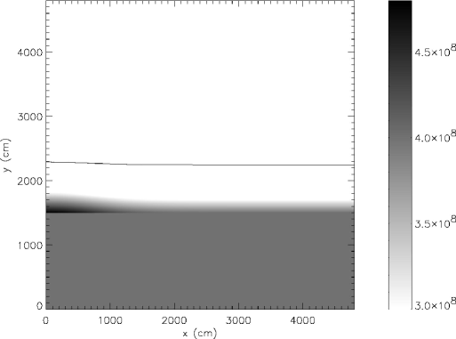
Figure 3.: Initial temperature perturbation. The black contour marks a density of $10\ \rm{g\ cm^{-3}}$, indicating the top of the initial atmosphere.

The temperature at the base of the fuel layer is perturbed with a Gaussian profile,

$$T(y)=T_{\rm{ash}}+(T_{\rm{perturb}}-T_{\rm{ash}})\cdot\exp\{-(y/L)^{2}\}$$ (6)

We integrate the equation of HSE outward from the fuel/ash interface using a second-order polynomial reconstruction for the zone-averaged density and a third-order reconstruction for the pressure:

$$\left<P\right>_{+1}-\left<P\right>_{0}=\frac{g\delta}{12}\left(5\left<\rho\right>_{+1}+8\left<\rho\right>_{0}-\left<\rho\right>_{-1}\right)$$ (7)

where $\delta$ is the zone width, and $\left<P\right>_{0}$ represents the average value of the pressure in zone 0. This reconstruction greatly suppresses any transients when an unperturbed model is evolved on our grid.

Figure 2 shows the vertical structure of the initial models at the maximally perturbed base temperature. Each column of our computational domain is given a unique initial model, according to the fuel base temperature specified by Eq. (6). The material up to the base of the fuel layer is in lateral pressure equilibrium. Figure 3 shows the temperature perturbation in the initial model (with a peak temperature of $4.8\times 10^{8}\ \rm{K}$) We note that there is only a pressure gradient in the $y$ direction in the fuel layer.

5. Computational Method

The calculations were performed with the FLASH code (Fryxell et al. 2000), solving the Euler equations with the piecewise-parabolic method (PPM) (Colella & Woodward 1984). Cylindrical geometry ($r$, $z$) were used to exploit the axisymmetric symmetry of the problem. Modifications to PPM were made to better evolve a hydrostatic atmosphere, and are discussed in Zingale et al. (2002). We use a Helmholtz free energy based tabular equation of state (Timmes & Swesty 2000), which allows for degenerate/relativistic electrons. No burning was used for these calculations—we only wish to determine the hydrodynamical effects.

The accurate solution of the spreading problem requires us to extend the physics of the atmosphere into the boundary conditions. In the absence of any perturbations, the Euler equations reduce to the condition of hydrostatic equilibrium. When the flow is hydrostatic, the boundary conditions are very influential. We use a hydrostatic boundary at the base of our model that provides pressure support to the material above it, while allowing sound waves to flow out. The material velocities are reflected in the boundary and the temperature is held constant. The density and pressure in the boundary are computed using the second-order zone-averaged differencing of HSE Eq. (7) coupled with the EOS (see Zingale et al. 2002).

At the upper boundary, we extend the domain for several 10s of meters above the surface of the atmosphere, to allow for the differences in the pressure scale heights of the perturbed and unperturbed regions. The density of this material above the atmosphere is small so as not to be dynamically important.

6. Results

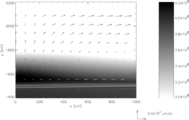
Figure 4.: Temperature (grayscale) and velocity (vectors) structure after 30 ns for the 20% perturbation.

We ran 3 different temperature perturbation simulations, 5%, 10%, and 20% (corresponding to 1.6%, 3.2%, and 6.4% pressure perturbations). Shortly after the simulation begins, a roll develops, with material comings towards the symmetry axis on the bottom, and flowing away on the top. This is shown in Figure 4 for the 20% temperature perturbation. The maximum spreading velocity we find as a function of time is shown in Figure 5. We see that, as expected, the spreading speed is greatest for the largest perturbation. It is difficult to determine from the data whether it follows the $(\delta P)^{1/2}$ dependence that we estimated in §3.

Figure 6 shows the maximum temperature on the grid as a function of time for the 3 runs. We expect the burning to be most vigorous at the peak temperature on the grid at any time, so this is in effect a measure of the nuclear timescales. Recall that in all cases, the ambient temperature is $4\times 10^{8}\ \rm{K}$. We see that in all cases, the temperature decreases very rapidly down to a level slightly higher than the background. In some instances, it even appears to increase slightly at long times—the reason for this is not known presently. The timescales of the decrease is $\sim 10s\ \mu s$—much faster than the nuclear timescale, and in agreement with our estimates in §3.

All of these estimates are much faster than the burning timescale, so this perturbation is unlikely to result in localized ignition. We can try longer perturbations—but the maximum length is the circumference of the star. Work is underway to generalize these results for different densities and perturbation sizes to determine whether a set of initial conditions exist under which we can locally burning the accreted fuel on a non-rotating neutron star.

These simulations were carried out with FLASH 2.1 (http://flash.uchicago.edu/). Support for this work was provided by the Scientific Discovery through Advanced Computing (SciDAC) program of the DOE, grant number DE-FC02-01ER41176. Some calculations we performed on the NERSC IBM SP/3 (seaborg) at LBNL.

Figure 5.: Maximum lateral velocity in the atmosphere as a function of time for the 3 different perturbations, 5% (lower), 10% (middle), and 20% (upper).

Figure 6.: Maximum temperature on the grid as a function of time for the 3 different initial models, 5% (lower), 10% (middle), and 20% (upper).

References

Colella, P. & Woodward, P. R. 1984, JCP, 54, 174

Cumming, A. 2002, this proceedings.

Fryxell, B. et al. 2000, ApJS, 131, 273

Fryxell, B. A. & Woosley, S. E. 1982, 261, 332

Spitkovsky, A., Levin, Y., & Ushomirsky, G. 2002, ApJ, 566, 1088

Timmes, F. X. & Swesty, F. D. 2000, ApJS, 126, 501

Zingale, M. et al. 2002, ApJS, accepted